Identification of a complete sample of northern ROSAT All-Sky
Survey X-ray sources

We present results of an investigation of the X-ray properties, age distribution, and kinematical characteristics of a high-galactic latitude sample of late-type field stars selected from the ROSAT All-Sky Survey (RASS). The sample comprises 254 RASS sources with optical counterparts of spectral types F to M distributed over six study areas located at $|b|\ga 20\degr$, and $DEC\geq-9\degr$. A detailed study was carried out for the subsample of $\sim$200 G, K, and M stars. Lithium abundances were determined for 179 G-M stars. Radial velocities were measured for most of the 141 G and K type stars of the sample. Combined with proper motions these data were used to study the age distribution and the kinematical properties of the sample. Based on the lithium abundances half of the G-K stars were found to be younger than the Hyades (660 Myr). About 25% are comparable in age to the Pleiades (100 Myr). A small subsample of 10 stars is younger than the Pleiades. They are therefore most likely pre-main sequence stars. Kinematically the PMS and Pleiades-type stars appear to form a group with space velocities close to the Castor moving group but clearly distinct from the Local Association.

1 Introduction

In a series of previous papers we reported about the results of a large programme on the optical identification of a complete count-rate limited sample of northern high-galactic latitude X-ray sources from the ROSAT All-Sky Survey (RASS) (Zickgraf et al. 1997a , 1997b , pap6 (1998), Appenzeller et al. pap3 (1998), 2000a , Krautter et al. pap4 (1999)). The sample was selected for the purpose of the investigation of the statistical composition of the high-galactic latitude part of the RASS in the northern hemisphere. As described in detail by Zickgraf et al. (1997a ) (hereafter Paper II) the selection criteria for the X-ray sources were X-ray count-rate and location in the sky. The sample is distributed in six study areas located at galactic latitudes $|b|\geq 20\degr$ and north of declination $-9\degr$. The optical identification was based on multi-object spectroscopy and direct CCD imaging. For more information on the identification process cf. Paper II. The catalogue of optical identifications and the statistical analysis of the sample were presented in Appenzeller et al. (pap3 (1998)) and Krautter et al. (pap4 (1999)) (hereafter Paper III and IV, respectively). We found that about 60% of the selected X-ray sources are extragalactic objects, i.e. AGN, clusters of galaxies, and individual galaxies. About 40% are stellar sources. Most of these (257 out of 274 objects) are F-M type coronal emitters. The rest are cataclysmic variables and white dwarfs. Follow-up investigations on the properties of subsamples formed by certain object classes were carried out for AGN (Appenzeller et al. 2000a ) and galaxy clusters (Appenzeller et al. 2000b ). A paper on the BL Lac objects in the sample is in preparation (Mujica et al.). The paper presented here is dedicated to the characteristics of the coronal stellar component.

A first discussion of the properties of the late-type stellar component was given by Zickgraf et al. (pap6 (1998)) (Paper VI). A subsample of stars in study area I located some $20\degr$ south of the Taurus-Auriga star forming region (SFR) was found to contain a large fraction of very young, presumably pre-main sequence stars. In order to investigate the age distribution of the complete sample of coronal X-ray emitters we obtained further low, medium and/or high resolution spectroscopic observations for most G-M stars in our sample. The goals were to carry out a lithium survey in order to identify lithium-rich high-galactic latitude G-M type stars and to determine precise radial velocities. In solar-like stars the lithium abundance can be used as an age estimator. Its knowledge therefore allows to study the age distribution of the X-ray active stellar sample. Combining the age information with proper motions and radial velocities would thus allow to investigate a possible age dependence of the kinematical properties of the stellar RASS sample.

This paper is structured as follows. The sample is presented in Sect. 2. Observations and data reduction are described in Sect. 3. Observational results are presented in Sect. 4. Based on these results the sample properties are analysed and discussed in Sect. 5. Finally, conclusions are given in Sect. 6.

Table 1: Journal of observations.

date	spectral res.	instrument	telescope
	$R=\lambda/\Delta\lambda$
Sep. 20-23, 1996	2 100	CAFOS	CA 2.2 m
Jan. 31 - Feb. 3, 1997	2 100	CAFOS	CA 2.2 m
Jan. 2-6, 1998	1 600	CAFOS	CA 2.2 m
Feb. 18, 1998	22 000	CASPEC	ESO 3.6 m
May 14-16, 1998	1 300	DFOSC	ESO Danish 1.54 m
Dec. 22-25, 1998	34 000	FOCES	CA 2.2 m
Apr. 29 - May 4, 1998	4 600	CARELEC	OHP 1.93 m
Oct. 21-16, 1998	20 000	AURELIE	OHP 1.52 m
Jan. 11-15, 2000	34 000	FOCES	CA 2.2 m
Jun. 13-18, 2000	34 000	FOCES	CA 2.2 m
Dec. 3-6, 2001	34 000	FOCES	CA 2.2 m
Feb. 19-23, 2002	34 000	FOCES	CA 2.2 m

2 The sample

2.1 Sample selection

Paper III presents a catalogue of optical identifications for 685 RASS sources contained in six study areas. The location of the study areas is plotted in Fig. 1 in galactic coordinates. The catalogue contains 254 X-ray sources which have been identified as coronal emitters of spectral types F to M. The contribution of the different spectral types is given in Table LABEL:revstat. One X-ray source, E020 = RXJ 1627.8+7042, was dropped from the stellar subsample. The star assigned as counterpart to this RASS source is too far from the X-ray position to be a plausible identification ($d=$ 1.5 arcmin). This source is more likely an optically faint AGN.

For the spectroscopic follow-up investigation we selected the 200 X-ray sources from the catalogue with stellar counterparts of spectral types G to M. F stars were not included in the spectroscopic follow-up observations because for these stars the lithium abundance is not a good age estimator. In 19 cases two stars have been assigned as counterpart to the X-ray source in Paper III. Several of these secondary counterparts were also observed. As in Paper IV we will however only use the primary identifications for statistical purposes. The entire “coronal” sample including the F type stars comprises 253 X-ray sources. The known RS CVn star HR 1099 (= V 711 Tau) which is X-ray source A031 in Paper III was excluded from the coronal sample discussed in the following. The sample finally selected for spectroscopic follow-up observations thus comprised 199 of the 200 X-ray sources with optical counterparts of spectral type G to M as listed in Paper III.

2.2 Photometry

Paper III gives visual magnitudes based mainly on photographic photometry from the Automated Plate Measuring (APM) machine (Irwin & McMahon IrwinMcMahon92 (1992)) except for stars with photometry listed in SIMBAD. Because the APM magnitudes lack a proper calibration their accuracy is rather low. We therefore obtained improved $V$ magnitudes by using photometry from other sources. Bright stars are contained in the Tycho-2 catalogue (Hog et al. Hogetal00 (2000)). For fainter stars not found in Tycho-2 magnitudes were taken either from the Hubble Guide Star Catalogue GSC-I (Lasker et al. Laskeretal90 (1990)) or for stars fainter than the limit of GSC-I from the GSC-II catalogue (The Guide Star Catalogue, Version 2.2.01). In a few cases no photometry is available because of blending with nearby neighbours. The Tycho-2 $V_{T}$ magnitudes were transformed to Johnson $V$ according to Mamajek et al. (Mamajeketal02 (2002)). GSC-I magnitudes were transformed to Johnson $V$ using the colour coefficients given in Russell et al. (Russelletal90 (1990)) and $B-V$ colours of main sequence stars for the corresponding spectral type taken from Schmidt-Kaler (SchmidtKaler82 (1982)). These colours were also used to calculate Johnson $V$ magnitudes from the GSC-II $B$ magnitudes. The improved $V$ magnitudes were then used to recalculate the ratio of X-ray-to-optical flux, $f_{\rm x}/f_{V}$, which is given in the Appendix in Table 13 together with other basic parameters of the sample stars.

Infrared photometry in $J,H,$ and $K$ was taken from the Two Micron All Sky Survey (2MASS) catalogue. From this data base infrared sources within 10″ around the optical position of the counterpart were extracted. A total of 267 2MASS sources was found of which 90% were located within 2″ from the optical counterparts (including the 19 double identifications, see above). We considered the 258 matches within 4″, i.e. within $3\sigma$ as reliable identifications. Matches between 4″  and 10″ were individually checked and all found to be also correct. This means that for all but 5 RASS sources (A035, A045, A065, D022, and D114) 2MASS measurements are available.

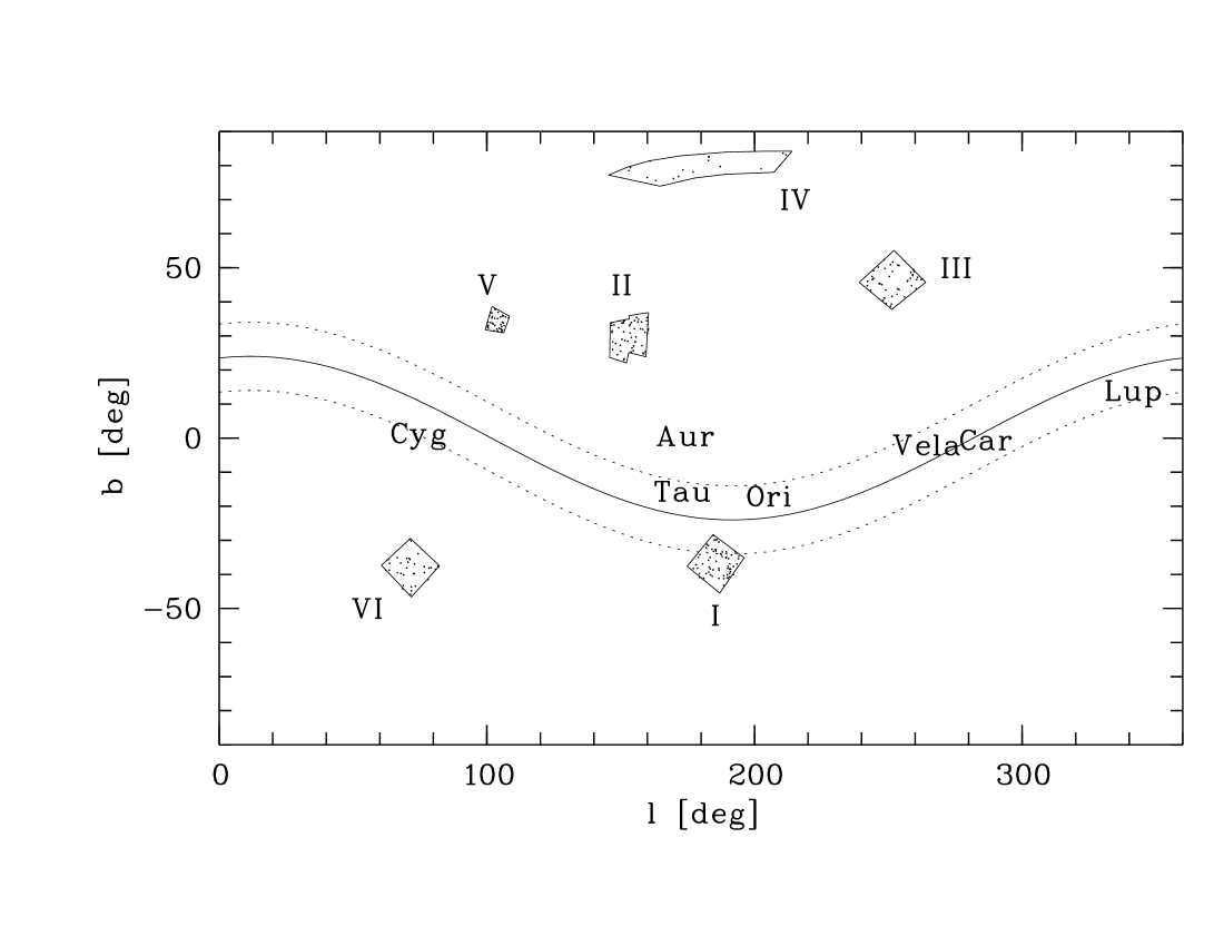
Figure 1: Location of the six study areas in galactic coordinates. The dots show the positions of the RASS X-ray sources with stellar counterparts in the respective area. The solid and dashed curves denote the position and width, respectively, of the Gould Belt according to Guillout et al. (Guilloutetal98 (1998)). In addition positions of several associations are shown.

3 Spectroscopic observations

The stellar sample of G to M above was observed spectroscopically during several observing runs. The journal of observations is given in Table 1. Low-resolution spectra were obtained with CAFOS, high-resolution spectra were observed with FOCES, both attached to the 2.2 m telescope at Calar Alto observatory (CA), Spain. Further high- and medium-resolution observations were obtained at the Observatoire de Haute Provence (OHP), France, with the spectrographs AURELIE and CARELEC at the 1.52 m and 1.93 m telescopes, respectively. A few supplementary high- and low-resolution observations were obtained at European Southern Observatory, La Silla, Chile (ESO), with CASPEC at the ESO 3.6 m telescope and DFOSC at the Danish 1.54 m telescope, respectively. A further observing run of 5 nights at Calar Alto observatory in February 2001 was lost due to bad weather conditions.

The spectra were reduced with the standard routines of the ESO-MIDAS software package. The low- and medium-resolution spectra and the high-resolution spectra observed with AURELIE were reduced with the Longslit package. For the FOCES and CASPEC data the routines of the Echelle package were applied.

Spectra could be secured for the counterpart of 172 out of 199 RASS sources with spectral types between G and M. High resolution observations were obtained for 118 of the 141 G and K stars of the selected sample (originally 143 G-K stars minus A031 and E020). Lithium equivalent widths and radial velocities for six of the stars not observed by us with high resolution were adopted from high-resolution spectroscopic studies by Wichmann et al. (Wichmannetal01 (2001)) (5 stars: A154, B049, B194, C062, C197) and Neuhäuser et al. (Neuhaeuseretal95 (1995)) (1 star: A058). Ten G-K stars fainter than 12th magnitude were observed only with low resolution. Thus for 134 of the 141 G-K stars spectroscopic follow-up observations exist. For the remaining 7 stars no observations could be obtained. Further high resolution data were found for the secondary counterpart of A098 in Favata et al. (Favataetal97 (1997)). With a few exceptions M stars were observed with low resolution only. Due to bad weather conditions during the OHP observing campaign the M stars in area V could not be observed. In total 38 M stars were observed with low resolution and 7 with high resolution. For 13 M stars no observations could be obtained.

In the following we give more technical details of the spectroscopic observations.

3.1 Low-resolution spectroscopy

For the low-resolution observations the focal reducer camera CAFOS attached to the 2.2 m telescope at Calar Alto observatory, Spain, was used during three observing runs. In 1996 and 1997 the instrument was equipped with a LORAL-80 2048$\times$2048 pixel CCD chip with a pixel size of 15$\mu$m. In 1998 a SITe1d 2048$\times$2048 pixel CCD chip with 24$\mu$m pixel size was used. Spectra in the wavelength range 4800–7450 Å were obtained (grism green-100) with a linear dispersion of 1.3 Å px^-1 and 2.1 Å px^-1 with the LORAL and the SITe1d CCD chip, respectively. With the LORAL chip the measured spectral resolution achieved with a 0.7″ slit was 3.2 Å ($FWHM$). The SITe1d chip and a 1″ slit yielded a spectral resolution of 4.2Å. Several stars were additionally observed in the blue wavelength region between 3850 Å and 5400 Å with the grism b-100 and a 1″ slit yielding similar spectral resolution as in the red wavelength range. Wavelength calibration was obtained using He and HgRb lamps. For flat-field correction spectra of the dome illuminated with a halogen lamp were recorded.

A few stars were observed in May 1998 with the focal reducer camera DFOSC attached to the Danish 1.54 m telescope at ESO, La Silla. The spectra were obtained with grism No. 7 and a slit width of 1″. The wavelength range covered by the spectra was 3840–6845 Å. As detector the LORAL/LESSER CCD# C1W7 with a pixel size of 15 $\mu$m was used. The resulting spectral resolving power was 1300.

3.2 Medium-resolution spectroscopy

In May 1998 medium-resolution spectra were obtained with the spectrograph CARELEC (Lemaître et al. Lemaitreetal90 (1990)) attached to the Cassegrain focus of the 1.93 m telescope at OHP. For the observations in the wavelength range from 6420 Å  to 6875 Å grating No. 2 with 1200 lines mm^-1 was used in 1st order with a TEK CCD chip (pixel size 27$\mu$m). The linear dispersion was 33Å mm^-1. The spectral resolution achieved was about 4600.

3.3 High-resolution spectroscopy

The largest part of the high-resolution observations were obtained during four observing campaigns with the echelle spectrograph FOCES (cf. Pfeiffer et al. Pfeifferetal98 (1998)) at the 2.2 m telescope of Calar Alto Observatory. The spectrograph was coupled to the telescope with the red fibre. The detector was a 1024$\times$1024 pixel Tektronix CCD chip with 24 $\mu$m pixel size. With a diaphragm diameter of 200 $\mu$m and an entrance slit width of 180 $\mu$m a spectral resolution of 34 000 was achieved. Wavelength calibration was obtained with a ThAr lamp. The nominal spectral coverage is from 3880Å to 6850Å. However, due to the wavelength dependence of the transmission curve of the red fiber and the continuum energy distribution of the stars the useful spectral range of the spectra is typically from $\sim 5000$Å to 6850Å. At shorter wavelength the S/N ratio decreases.

In October 1998 high-resolution spectra were obtained with the spectrograph AURELIE at the 1.52 m telescope of the OHP. A description of the spectrograph can be found in Gillet et al. (Gilletetal94 (1994)). The spectra were observed with grating No. 2 with 1200 lines mm^-1 giving a reciprocal linear dispersion of 8 Å mm^-1. The detector was a double-barrette Thomson TH7832 (2048 pixel with 13 $\mu$m pixel size). The spectra cover the wavelength interval from 6540 Å to 6740 Å. The resolution of the spectra is 20 000. Wavelength calibration was obtained with Neon and Argon lamps.

High-resolution spectra of 3 objects were obtained with the Cassegrain Echelle Spectrograph (CASPEC) at the ESO 3.6 m telescope on La Silla in February 1998. Wavelength calibration was obtained with a ThAr lamp. The CASPEC spectra cover the spectral range from 5350 to 7720 Å with a nominal resolving power of 22,000 (Sterzik et al. Sterziketal99 (1999)).

During each high-resolution observing campaign radial and rotational velocity standard stars were observed in addition to the science targets.

4 Observational results

4.1 Spectral classification

In Paper III spectral types were given based largely on low-resolution classification spectra obtained with LFOSC (cf. Paper II). For a smaller number of stars spectral types were adopted from the literature. Our high-resolution spectra not only allowed us to refine the classification but, even more importantly, enabled us to derive luminosity classes and hence spectroscopic parallaxes.

During the observing runs a small set of spectroscopic standard stars, mainly of luminosity class V, had been observed together with the science targets. The coverage of the spectral type - luminosity class plane, however, was insufficient for a detailed two-dimensional classification. We therefore extended the spectroscopic data base for the standard stars by making use of the spectra available in the stellar library of Prugniel & Soubiran (PrugnielSoubiran01 (2001)) which is part of the HYPERCAT data base. We used the data set with a spectral resolution of 10 000. In order to match this resolution our FOCES, AURELIE, and CASPEC spectra were smoothed accordingly with an appropriate Gaussian filter. In this way the signal-to-noise ratio improved while the necessary spectral resolution for the classification was preserved. Spectral types and luminosity classes (LCs) of MK standard stars contained in the stellar library were adopted from Yamashita et al. (Yamashitaetal76 (1976)), Keenan & McNeil (KeenanMcNeil89 (1989)), Garcia (Garcia89 (1989)), Keenan & Barnbaum (KeenanBarnbaum99 (1999)), and Gray et al. (Grayetal01 (2001)). In a few cases we adopted the spectral classification given in Prugniel & Soubiran (PrugnielSoubiran01 (2001)). The grid of spectroscopic standard stars is listed in Table 3.

In a pilot study for the work presented here Ziegler (Ziegler93 (1993)) studied the spectral types of F, G and K-type stars from the RASS using spectra observed in the red spectral region ($\lambda\lambda$6200 - 6750 Å). He found various line ratios useful for classification purposes. For the F- and G-type stars the ratios Fe i $\lambda$6394/Si ii $\lambda$ 6346, Fe ii$\lambda$6456/Ca i $\lambda$6450 and Fe ii$\lambda$6456/ Fe i $\lambda$6394 were found to be good indicators for the spectral type. In K stars the ratios TiO $\lambda$6240 / V i $\lambda$6296 and Fe i $\lambda$ 6250/Ca i $\lambda$6450 were useful classification criteria.

We used these ratios for the refinement of the spectral types given in Paper III. Figure 2 shows the histogram of the differences between the revised and original spectral types. The narrow peak shows that with few exceptions the overall agreement is good. We found a small mean difference of -0.5 subclass between the high- and low-resolution spectral types with a standard deviation of 2.2 subclasses. The original and the revised statistics of spectral types are listed in Table LABEL:revstat. In nine cases the difference of the spectral types was larger than $\pm 3$ subclasses. The largest differences were found for B174 and E256 ($-6$ subclasses), B185 (7 subclasses), D018 (9 subclasses), and E022 and E067 ($-9$ subclasses). The LFOSC spectrum of E256 was actually classified as K4, but erroneously entered in Paper III as M0. For D018 which is a very bright star the original LFOSC spectrum classified as G2V could suffer from saturation. In SIMBAD this star is listed as K0III (Schild Schild73 (1973)). The classification based on the FOCES spectrum is K1III, which is in good agreement with the literature. We adopt this spectral class in the following. For the remaining stars with large deviations no LFOSC classification spectra were obtained. The spectral classes were adopted from SIMBAD. In the following we use the improved FOCES classifications.

Table 2: Revised and original statistics of the distribution of spectral type among the RASS sources with stellar counterparts of spectral types F to M.

spec. type	this work	Paper IV
F	55	53
G	56	54
K	86	89
M	56	58
total	253	254

Following Gahm & Hultqvist (GahmHultqvist72 (1972)) and Ziegler (Ziegler93 (1993)) luminosity classes (LC) were obtained using the strength of the lines of Ba ii $\lambda\lambda$5854Å, 6497Å, Sc ii $\lambda$6605Å, and La ii $\lambda$6390Å. We added the Y ii $\lambda$6614Å line which also shows a clear luminosity dependence. The ratio of Sc ii $\lambda$6605Å and Y ii $\lambda$6614Å is a good luminosity indicator for spectral types earlier than about K5-7. For spectral types later than K0 the strength of La ii  was additionally useful to discriminate luminosity classes III and higher from LC V and IV. For G stars LC III and higher could also be discriminated from LC IV by the use of this line. Comparing in this way the line strengths and ratios in the MK standards with the sample stars LCs could be assigned to most stars. For a few stars the stellar absorption lines were strongly broadened by rapid rotation (see below). In these cases it was not possible to determine the luminosity class due to the limited S/N of the spectra and to line blending. The limit was reached around $v\sin i\ga 30$ km s^-1. For the rapid rotators we adopted LC V. As discussed in Sect. 5.1.1 we used the luminosity classes to derive spectroscopic parallaxes.

Table 3: Spectroscopic MK standard stars. The spectral types are listed in column “sp. type”. References for the spectral types are given in column “ref.”: 1 = Yamashita et al. (Yamashitaetal76 (1976)), 2 = Gray et al. (Grayetal01 (2001)), 3 = Keenan & Barnbaum (KeenanBarnbaum99 (1999)), 4 = Garcia (Garcia89 (1989)), 5 = Keenan & McNeil (KeenanMcNeil89 (1989)), 6 = Prugniel & Soubiran (PrugnielSoubiran01 (2001)).

star	sp. type	ref.	star	sp. type	ref.
HD 222368	F7V	4	HD 188119	G7III	4
HD 016765	F7IV	6	HD 010700	G8V	4
HD 216385	F7IV	6	HD 188512	G8IV	4
HD 181214	F8III	6	HD 027348	G8III	3
HD 004614	G0V	4	HD 175306	G9III	4
HD 013974	G0V	4	HD 145675	K0V	5
HD 019373	G0V	4	HD 185144	K0V	4
HD 114710	G0V	1	HD 198149	K0IV	5
HD 150680	G0IV	4	HD 048433	K0III	3
HD 039833	G0III	6	HD 010476	K1V	5
HD 204867	G0Ib	1	HD 222404	K1IV	5
HD 204613	G1III	4	HD 096833	K1III	5
HD 185758	G1II	4	HD 022049	K2V	4
HD 186408	G2V	4	HD 137759	K2III	4
HD 126868	G2IV	2	HD 020468	K2II	4
HD 209750	G2Ib	1	HD 219134	K3V	4
HD 117176	G4V	5	HD 003712	K3III	3
HD 127243	G4IV	5	HD 201091	K5V	4
HD 186427	G5V	1	HD 118096	K5IV	6
HD 161797	G5IV	4	HD 029139	K5III	3
HD 027022	G5IIb	5	HD 088230	K6V	4
HD 206859	G5Ib	1	HD 201092	K7V	4
HD 003546	G6III	5	HD 079210	M0V	6
HD 182572	G7IV	4	HD 046784	M0III	6

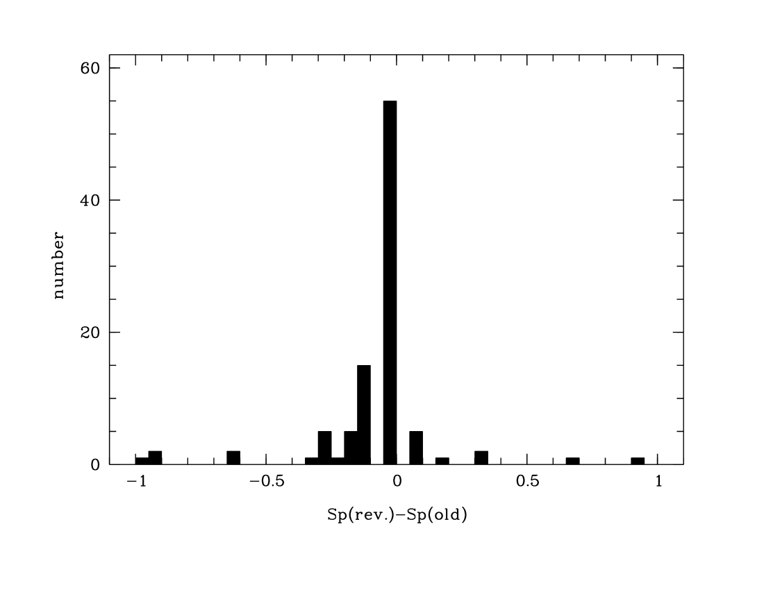
Figure 2: Comparison of the spectral types derived from the classification spectra used in Paper III (Sp(old)) and from the new high resolution spectra (Sp(rev.)). The abscissa is the difference (in spectral classes) between the revised and the original spectral types.

4.2 Radial and rotational velocities

During each observing run for high-resolution spectroscopy a set of radial and rotational velocity standards had been observed together with the RASS counterparts. Heliocentric radial velocities were measured by means of a cross-correlation method (Simkin Simkin74 (1974)). The continuum was subtracted from the normalized spectra which were then rebinned on a logarithmic wavelength scale. The shift relative to the radial velocity standards was measured and transformed into the radial velocity of the target by taking into account the radial velocity of the standard stars. The individual radial velocities obtained for each standard star were averaged to give the final result. The standard deviation gives a measure for the error. With few exceptions (spectra with low S/N and/or high rotational velocity) the errors were in the range 1-4 km s^-1 with a typical error of about 2-3 km s^-1. Heliocentric radial velocities (and errors) are listed in Table 14.

The width of the cross-correlation function is a measure for the rotational velocity $v\,\sin i$. We therefore calculated the cross-correlation function as before but for rotational velocity standards. Standard stars with low $v\,\sin i$ and spectral type as close as possible to that of the objects were used for the cross-correlation analysis as well as to calibrate the FWHM vs. $v\,\sin i$ relation. From the FWHM of the cross-correlation function $v\,\sin i$ was then determined following the method described in Covino et al. (Covinoetal97 (1997)). Observations of rotational standard stars yielded a detection limit of $v\,\sin i$ of about 5 km s^-1. From the statistics of the differences between measured rotational velocities of rotational standard stars and $v\,\sin i$ from the literature an uncertainty of $v\,\sin i$ of 3 km s^-1 could be estimated. For rotational velocities above $\sim 40$ km s^-1 the shape of the peak of the correlation function deviates increasingly from a Gaussian leading to larger errors of 5-10 km s^-1. Figure 3 shows the histogram of the rotational velocities which are listed in Table 13.

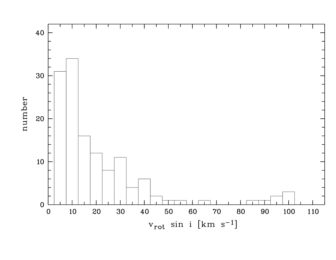
Figure 3: Distribution of rotational velocities of the G and K stars.

4.3 Lithium equivalent widths

Equivalent widths (EWs) of the lithium absorption line Li i $\lambda 6708$, $W$(Li i ) were determined from the low-, medium- and high-resolution spectra. The measurement of the EW in the low- and medium resolution spectra was performed as described in detail in Paper VI. Essentially, the method takes the line blending with neighboring Fe i  lines into account by fitting Gaussian profiles at the wavelengths of the Fe i  lines at 6703, 6705, and 6710 Å simultaneously with the lithium line at 6708Å. In Paper VI the error of $W$(Li i ) determined from the CAFOS spectra was estimated to be about 60 mÅ. For the DFOSC spectra the uncertainty is similar. The fitting procedure was also applied to the medium-resolution CARELEC spectra. The uncertainty of the EW for these spectra is about 40 mÅ.

In the high-resolution spectra the equivalent widths were measured directly by integrating the flux in the normalized spectra. The contribution of the neutral iron line Fe i $\lambda 6707.441$Å was corrected according to the procedure described by Soderblom et al. (1993b ). For stars with rotational velocities larger than $\sim 30$ km s^-1 the contribution of the Fe i  lines near Li i $\lambda 6708$ was corrected in the following way. From the stellar library of Prugniel & Soubiran a spectroscopic standard star with a spectral type as close as possible to the target was selected. It was folded with the appropriate rotational velocity to match the broadened lines of the target spectrum. Then the EW of the Fe i  absorption features was measured in the same wavelength interval as used to determine the Li i  EW in the target spectrum. Finally the corrected lithium EW was obtained by subtracting the contribution of the Fe i  lines from the measured lithium EW of the target spectrum. Errors of the high-resolution EWs are typically 5-15 mÅ, depending on the signal-to-noise ratio and on the rotational velocity. The EWs are listed in Table 15.

In Fig. 4 the EWs obtained from the low- and the high-resolution spectra are compared. In the low-resolution spectra the EWs $W$(Li i ) are obviously slightly underestimated by about 40 mÅ. However, the overall agreement is good and the differences are only of the order the uncertainty of the low-resolution measurements. This demonstrates that the fitting method applied to the low-resolution spectra works remarkably well. In particular, $W$(Li i ) is not overestimated as it would be the case if the EWs would be determined directly by flux integration without taking the contribution of the Fe i  lines into account.

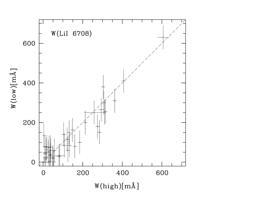
Figure 4: Comparison of the equivalent widths of Li i  determined from the low- and the high-resolution spectra. The dashed line denotes a ratio of 1 of the two measurements.

4.4 Binaries

Spectroscopic binaries were detected by means of the shape of the cross-correlation function obtained for the radial velocity determination. Among the 125 G-K stars with high-resolution spectroscopy either obtained by us or taken from the literature 32 binary systems and 1 triple system were found. The triple system is B160. The fraction of multiple systems in our sample of G-K type stars with high-resolution observations thus is 26% with a lower limit of 23% for the full sample of G-K stars.

In a few binaries lithium lines could be identified in one or both components. In order to disentangle the lines of the individual components and to identify a possible Li i  line spectra from the Prugniel & Soubiran sample with the appropriate spectral types were folded with the rotational profile for the measured $v\,sini$ and shifted with respect to the measured radial velocities. Then the spectra were superimposed by using appropriate values for the relative flux contributions. Finally the resulting artificial binary spectrum was compared with the observed spectrum. Correction factors for the measured lithium equivalent widths were estimated from the artifical spectrum. In most cases the spectra suggest a flux ratio of 1 to 2 for the individual components at 6708 Å. Exceptions are e.g. A001 and A071. In A001 the primary component is a fast rotator ($v\,sini\approx 100$ km s^-1) whose broad lines dominate the spectrum. Of the secondary component only the strongest lines of a mid to late type K star are detectable. For this binary system we adopted a flux ratio of 5:1 for the continuum contributions of the primary and secondary component at 6708 Å. In A071 both components are fast rotators with very broad lines. In this case it was not possible to determine a lithium EW for each component. The total EW was therefore assigned in equal shares to the individual components and the lithium equivalent widths were corrected by assuming equal flux contributions. The triple system B160 is even more complicated. It consists of 3 early to mid G-type stars with spectral types between $\sim$G2 and $\sim$G5. Two of the three components exhibit a lithium absorption line.

It is clear that the equivalent widths of the binaries and the triple system are less reliable than those of the single stars due to the uncertainty of the continuum correction. In Table 15 the lithium EW of the strongest component is given.

5 Data analysis and discussion

In the following we will first discuss the basic parameters of the coronal sample and then investigate the age distribution using lithium abundances, and the kinematics as derived from radial velocities and proper motions.

5.1 Basic properties

5.1.1 Distances

The distance is clearly one of the most important parameters. For 58 of the 252 F-M type counterparts a Hipparcos parallax with $\pi_{\rm H}/\sigma_{\rm H}\geq 3$ exists. The 58 stars with Hipparcos parallax comprise 28 F stars, 17 G stars, 9 K stars and 4 M stars. Further trigonometric parallaxes of 7 M stars were found in Gliese & Jahreiss (GlieseJahreiss91 (1991)).

For 74 stars a spectroscopic parallax could be derived from the high-resolution spectra by adopting the absolute $V$ magnitudes, as appropriate for the spectroscopically determined luminosity class, from Schmidt-Kaler (SchmidtKaler82 (1982)). For the bulk of M stars we used infrared $JHK$ measurements from the 2MASS catalogue to derive a photometric distance. The two-colour diagram of $J-H$ and $H-K$ is displayed in Fig. 5. It shows that the M stars are distributed around the locus of main-sequence stars (solid line in Fig.5). For the further analysis distances of M stars were therefore estimated by adopting $M_{V}$ for LC V from Schmidt-Kaler (except for the 11 stars with trigonometric parallaxes). This adds 43 more RASS sources with a distance estimate. Thus total distances are available for 100 G-K and 54 M stars. For the remaining stars without a distance measurement we derived a lower limit for the distance by assuming that they are main-sequence objects with LC V.

An estimate of the error of the spectroscopic and photometric distances, $\sigma_{d}$, may be obtained from the following considerations. The error is due to the uncertainties of the absolute visual magnitude, $M_{V}$, and of $V$. For the latter we conservatively adopted the error of the photographic GSC magnitudes $\sigma_{V}=0.3^{\rm m}$ for all stars. The dominating source of uncertainty is the error of $M_{V}$. For G-K stars of LC V and IV and correspondingly for LC III and II we used half of the difference of $M_{V}$ of these luminosity classes as estimate for $\sigma_{M_{V}}$. This leads to an estimate for $\sigma_{d}/d$ of 30-50%. In the case of M stars the main source of error of $M_{V}$ is due to the uncertainty of the spectral class. This also leads in total to $\sigma_{d}/d\sim$50% if an uncertainty of 1-2 spectral subclasses is assumed. We finally adopted 50% as relative error for spectroscopic and photometric distances.

For the derivation of the distances interstellar extinction was not taken into account. Given the high galactic latitude of our sample it is actually expected to be small. With the relation $N_{H}=5.9\,10^{21}\times E(B-V)$ given by Spitzer (Spitzer78 (1978)) with the column density of neutral hydrogen, $N_{H}$, and colour excess $E(B-V)$ upper limits of the extinction can be estimated. We expect extinction values, $A_{V}$, of less than 0.2-0.3 in all study areas except area I. This region could have a higher extinction of up to 0.6 magnitudes for the most distant stars. For these estimates the $N_{H}$ values given in Paper II were used.

For 20 stars in our sample both spectroscopic and Hipparcos parallaxes, $\pi_{\rm H}$, exist. They are compared in Fig. 6. The agreement of the two distance measurements for this subsample is good. The mean ratio of both parallaxes is $1.06\pm 0.35$. For the further analysis we adopted the spectroscopic parallaxes if no Hipparcos parallax with $\pi_{\rm H}/\sigma_{\pi}>3$ or other trigonometric parallax was available. The adopted distances are listed in Table 13.

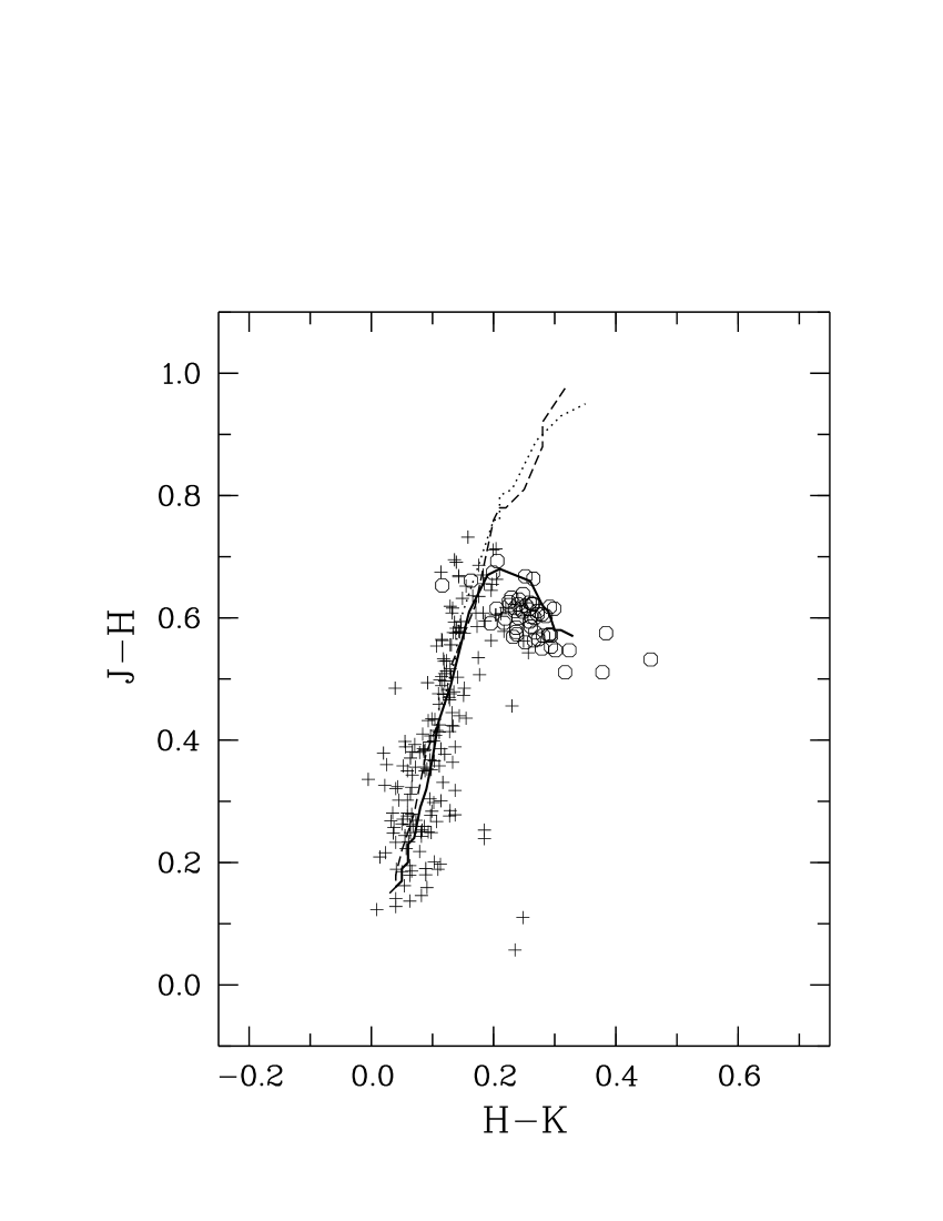
Figure 5: Two-colour diagram for the infrared magnitudes from 2MASS. Circles denote M stars, crosses stars with spectral types F to K. The solid, dotted, and dashed lines denote the loci of main sequence stars, giants, and supergiants, respectively.

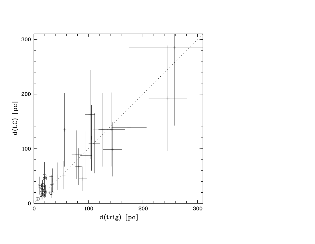
Figure 6: Comparison of the distances $d({\rm LC})$ derived from spectroscopic or photometric parallaxes and from trigonometric parallaxes, $d({\rm trig})$. The dashed line denotes equal distance values. M stars with distance estimates from the 2MASS IR photometry are plotted as circles.

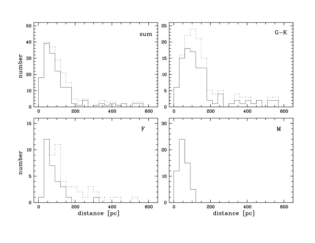
Figure 7: Histogram of the distance distribution. The solid lines represent the distribution of trigonometric, spectroscopic, and photometric parallaxes. The dashed lines include distance estimates derived from assuming absolute visual magnitude of main-sequence stars for the remaining stars without other distance estimate.

Figure 7 shows the number distribution of the distances for the 184 F-, G-, and M stars. Also shown is the distribution including the stars with minimum distances estimated by adopting LC V. The number distribution of the total sample has a maximum around 50 pc with a tail extending up to several 100 pc. Most stars are nearer than 200 pc, 33 stars have distances above 300 pc (including 16 stars with minimum distances), and in 4 cases (not shown in Fig. 7) we derived a distance above 1 kpc (including 3 stars with minimum distances). The identifications of the very distant RASS counterparts may be questionable.

For the stars with trigonometric parallaxes the absolute magnitude, $M_{V}$, was calculated from the distance and visual magnitude given in Table 13. A luminosity class was then assigned according to Schmidt-Kaler (SchmidtKaler82 (1982)). Likewise, bolometric corrections were taken from the same reference to determine the bolometric magnitudes for all stars with known distances.

As expected the majority of stars with a luminosity class determination, $\sim$90%, have luminosity class V or IV. A small number of 17 stars was classified as giants (LC III-IV, III, and II), 12 of these based on Hipparcos parallaxes. In Fig. 8 the H-R diagram is shown for all stars with a spectroscopic or trigonometric parallax. M stars are shown only if a trigonometric parallax was available.

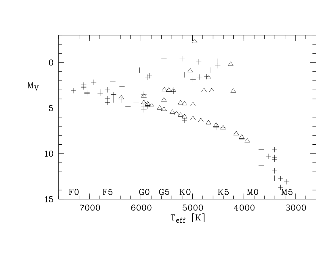
Figure 8: H-R-diagram for single stars with either a trigonometric parallax from Hipparcos or other sources ($+$ sign) or with a spectroscopic parallax (triangles).

5.1.2 X-ray properties

In Paper II we discussed the X-ray flux limits in the ROSAT 0.1–2.4 keV energy band for the various classes of X-ray emitters in our sample. For coronal emitters it is 2 10^-13 erg cm^-2 s^-1. An exception is study area V which due to the deeper RASS exposure near the north ecliptic pole has a lower flux limit of 0.6 10^-13 erg cm^-2 s^-1. X-ray luminosities, $L_{\rm X}$, were derived from the fluxes given in Paper III and the distances derived here. In Fig. 9 $L_{\rm X}$ is plotted vs. the distance. Also shown are the two flux limits. As expected for a flux-limited sample this plot shows a correlation between distance and luminosity because at increasingly larger distances only the more luminous objects are detected.

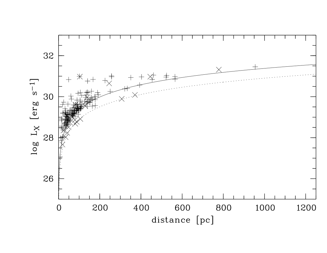
Figure 9: X-ray luminosity for single stars vs. distance. $+$ signs mark stars in study areas I, II, III, IV, and VI, $\times$ signs represent stars in area V. The solid and dotted lines mark the flux limits for the two groups of study areas.

In Fig. 10 $L_{\rm X}$ is plotted versus the effective temperature and Fig. 11 shows $L_{\rm X}$ as function of the absolute visual magnitude, $M_{V}$. A weak trend of $L_{\rm X}$ increasing with increasing $T_{\rm eff}$ is visible. The $L_{\rm X}$-$M_{V}$ diagram shows a clear correlation with $L_{\rm X}$ decreasing for decreasing optical luminosity. This reflects the fact that $L_{\rm X}$ depends on the emitting surface. The width of the $L_{\rm X}$-$M_{V}$ distribution at a given $M_{V}$ tells that the X-ray surface flux density of the stars in our sample spans a range of a factor of $\sim 1000$. Around $M_{V}=5$ the lower limit of the X-ray luminosities of the sample stars is about a factor of 10 above the solar soft X-ray variability range ($5\,10^{26}-2\,10^{27}$ erg s^-1, Schmitt Schmitt97 (1997)). The upper limit of $L_{\rm X}$ in our sample is about a factor of 10-30 higher than in the volume-limited sample of Schmitt (Schmitt97 (1997)).

The ratio of $L_{\rm X}$ and bolometric luminosity, $L_{\rm bol}$, is plotted in Fig. 12 as function of $M_{\rm bol}$. A clear correlation is visible with the low luminosity stars with later spectral types having the highest ratio of $L_{\rm X}/L_{\rm bol}$. This is in agreement with the results of Fleming et al. (Flemingetal95 (1995)) who studied the coronal X-ray activity of low-mass stars in a volume limited sample. They found the highest ratios of $L_{\rm X}/L_{\rm bol}$ for dMe stars. As discussed in Paper IV, most M stars in our sample are actually dMe stars, that is of the 58 M stars listed originally in Paper III 53 exhibit H$\alpha$ emission lines. Note, however, that selection effects inherent in our flux-limited sample may also play a role.

The X-ray surface flux density is displayed as a function of $M_{V}$ in Fig. 13 and as a function of $T_{\rm eff}$ in Fig. 14. Our sample contains mainly stars with a high surface flux density which is on the average 1 to 2 orders of magnitude above the solar flux level. This can be understood in view of the result discussed below in Sect. 5.2.2 that our sample contains a large fraction of young and hence very X-ray active stars. Old solar-like stars are obviously not present in our sample. The maximum value of the surface flux density of our sample stars is around $10^{8}$ erg s^-1 cm^-2. This value is consistent with the result obtained by Schmitt (Schmitt97 (1997)) who found a maximum around $10^{7}-10^{8}$ erg s^-1 cm^-2 in his volume-limited sample of solar-like stars.

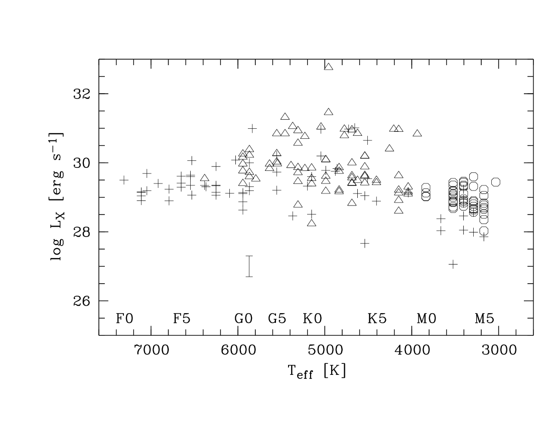
Figure 10: X-ray luminosity for single stars as a function of effective temperature, $T_{\rm eff}$. Different symbols identify stars with trigonometric ($+$ sign), spectroscopic (triangles), or IR photometric parallaxes (circles). The variability range of solar X-ray emission in the ROSAT-PSPC pass band is marked by the vertical bar.

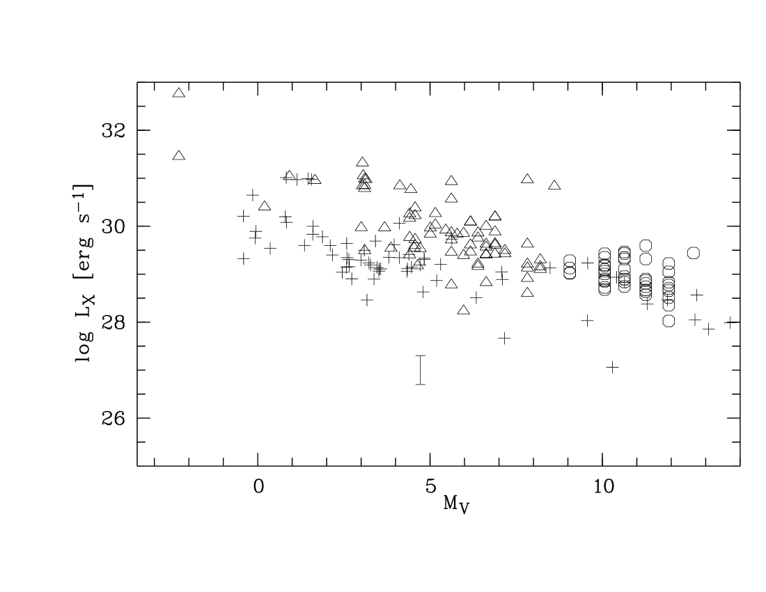
Figure 11: X-ray luminosity for all single stars with trigonometric ($+$ sign), spectroscopic (triangles), or IR photometric parallaxes (circles) as a function of absolute visual magnitude, $M_{V}$. The variability range of solar X-ray emission is marked by the vertical bar.

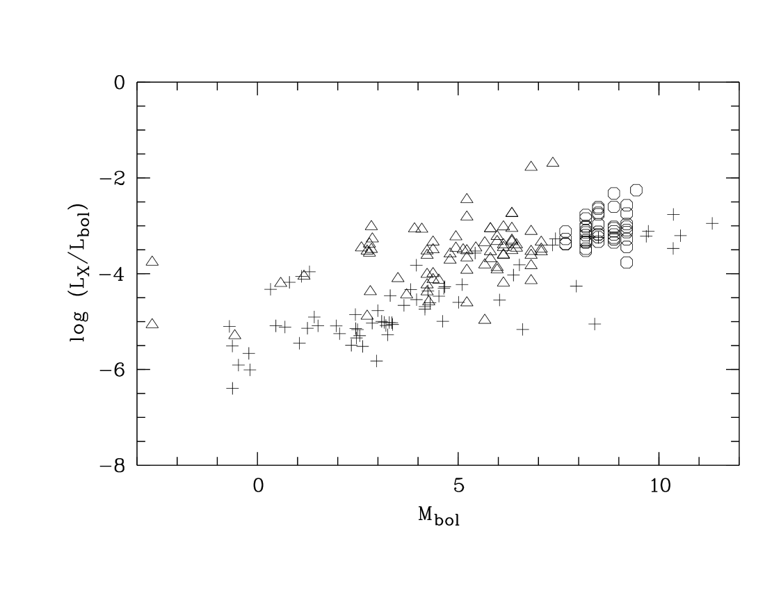
Figure 12: Ratio of X-ray and bolometric luminosity for all single stars with trigonometric ($+$ sign), spectroscopic (triangles), or IR photometric parallaxes (circles) as a function of bolometric magnitude, $M_{\rm bol}$.

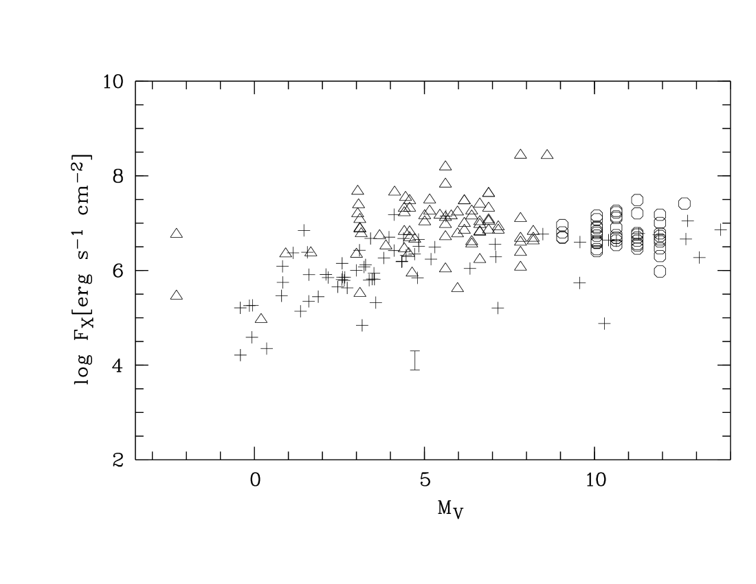
Figure 13: X-ray surface flux density for all single stars with trigonometric ($+$ sign), spectroscopic (triangles), or IR photometric parallaxes (circles) as a function of absolute visual magnitude, $M_{V}$. The vertical bar marks the typical flux level of solar coronal holes in the ROSAT-PSPC pass band.

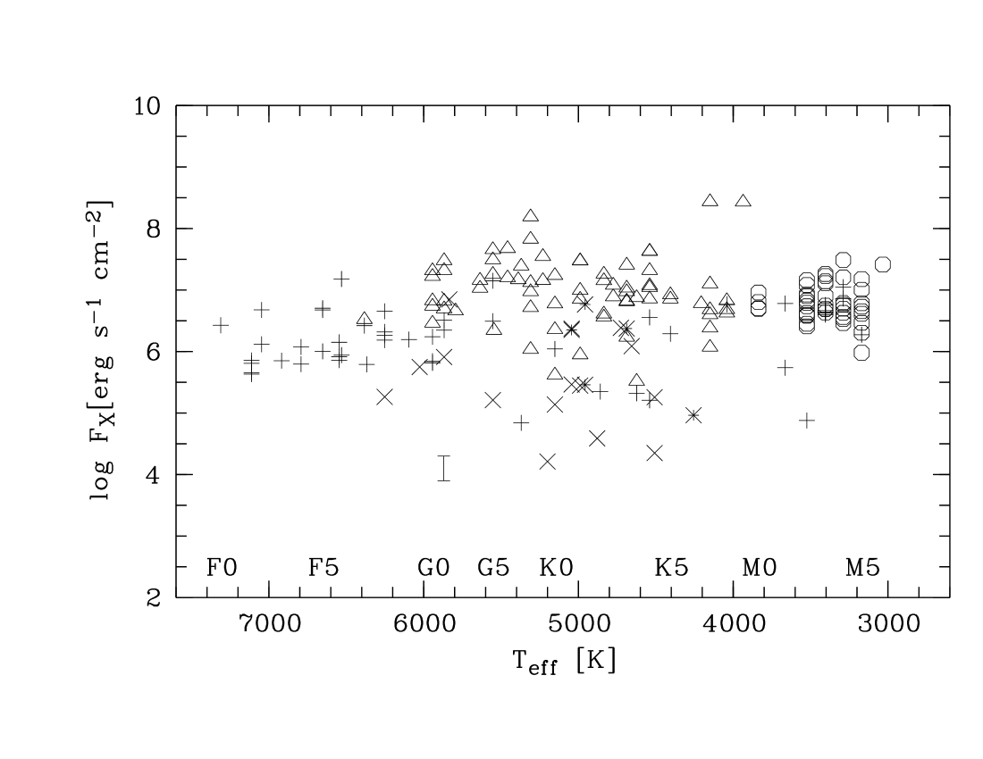
Figure 14: X-ray surface flux density for all single stars as a function of effective temperature, $T_{\rm eff}$. The meaning of the symbols is the same as in Fig. 10. The vertical bar marks the typical flux level of solar coronal holes in the ROSAT-PSPC pass band.

Finally, in Fig. 15 the ratio $\log L_{X}/L_{\rm bol}$ is displayed as function of projected rotational velocity, $v\,\sin\leavevmode\nobreak\ i$. No clear correlation can be seen, except that small ratios of $\log L_{X}/L_{\rm bol}$ are only found for small $v\,\sin\leavevmode\nobreak\ i$, whereas fast rotators exhibit high $\log L_{X}/L_{\rm bol}$ ratios.

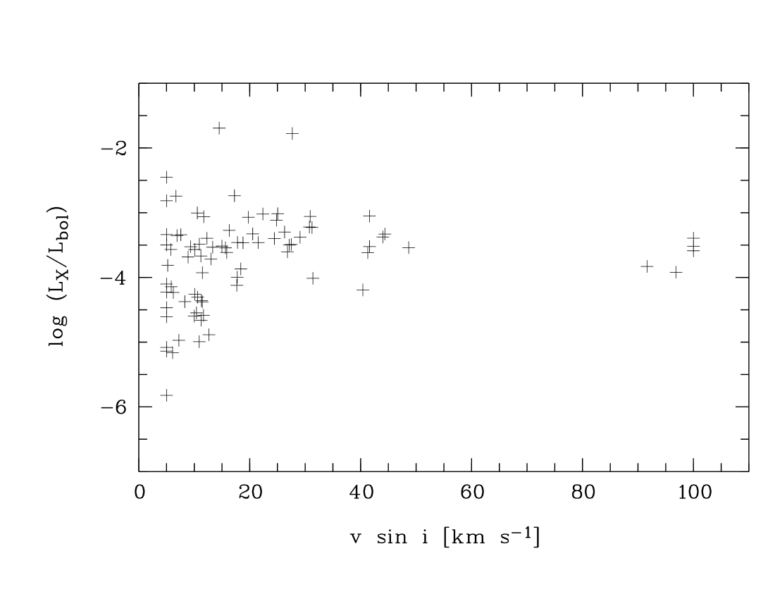
Figure 15: $\log L_{X}/L_{\rm bol}$ as a function of $v\,\sin i$.

5.2 Lithium abundances and age distribution

5.2.1 Lithium abundances

The spectroscopic survey resulted in the detection of significant Li i  absorption lines in a large fraction of the G and K stars in our sample. In 51 G-K stars lithium absorption lines with an EW larger than 60 Å were found. The number of lithium-rich M-type stars is very small. We found significant Li i  absorption lines in only 2 out of 47 observed M stars. In Fig. 16 the EWs of Li i $\lambda 6708$ Å  are plotted versus $T_{\rm eff}$ for the entire sample. In Fig. 24 in the Appendix the same plots are shown for the individual study areas.

The lithium equivalent widths were converted to abundances, $N$(Li), by using the curves of growth of Soderblom et al. (1993b ) for stars with $T_{\rm eff}>4000$ K and of Pavlenko & Magazzù (PavlenkoMagazzu96 (1996)) and Pavlenko et al. (Pavlenkoetal95 (1995)) for cooler stars. As in Paper VI effective temperatures were derived from the spectral types using the temperature calibrations of de Jager & Nieuwenhuijzen (deJagerNieuwenhuijzen87 (1987)). The uncertainty of $T_{\rm eff}$ is typically 200 K. This leads to errors of the estimated Li abundances of about 0.3 dex. Lithium abundances are shown in Fig. 17 as function of effective temperature with $v\,\sin\leavevmode\nobreak\ i$ indicated by the symbol size.

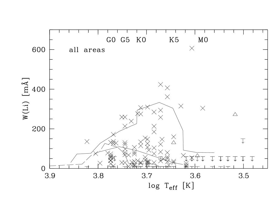
Figure 16: Equivalent widths of Li i $\lambda 6708$ as a function of $T_{\rm eff}$ for all stars in the six study areas. Crosses and triangles are high and low resolution measurements, respectively. The solid lines represent the upper and lower envelope of the lithium equivalent widths in the Pleiades adopted from Soderblom et al. (1993b ). The dashed line shows the upper envelope for the Hyades cluster taken from Thorburn et al. (Thorburnetal93 (1993)).

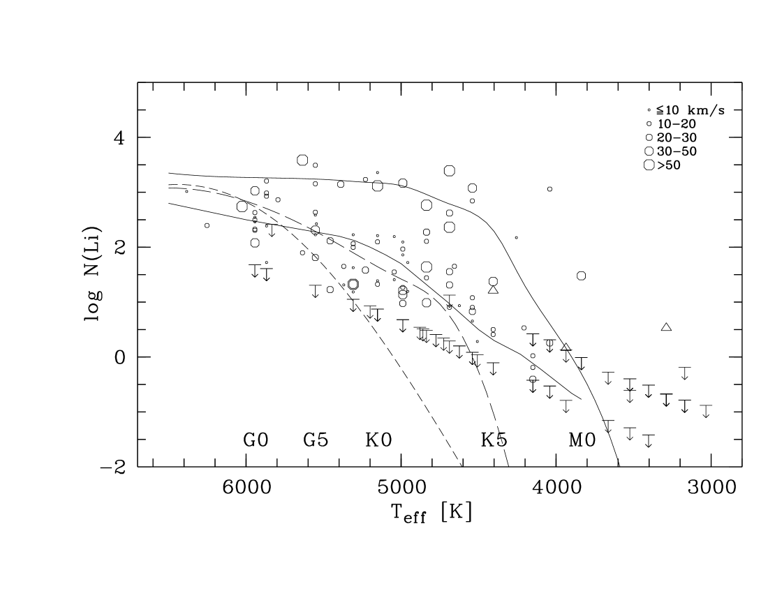
Figure 17: Lithium abundances versus effective temperature for the complete sample. Upper limits are plotted as downward arrows. Circles denote high-resolution measurements with the symbol size depending on $v\,\sin i$. Low and medium resolution data are plotted as triangles. The solid lines are the upper and lower limit of $\log N$(Li i ) in the Pleiades; the long dashed and short dashed lines show the upper $\log N$(Li i ) limits for the UMaG and the Hyades, respectively.

5.2.2 Classification of age groups

In order to obtain information about the age distribution of the sample stars we compared our lithium measurements with the corresponding measurements of stars in clusters with various ages: IC 2602 (30 Myr), the Pleiades (100 Myr), M 34 (200 Myr), the Ursa Major group (UMaG, 300 Myr), and the Hyades (660 Myr). Ages are from Lang (Lang92 (1992)) except for IC 2602 for which we adopted the age given by Stauffer et al. (Staufferetal97 (1997)). The lithium data were taken from Randich et al. (Randichetal97 (1997)) for IC 2602, Soderblom et al. (1993b ) for the Pleiades, Jones et al. (Jonesetal97 (1997)) for M 34, Soderblom et al. (1993a ) for UMaG, and Thorburn et al. (Thorburnetal93 (1993)) for the Hyades. Note that these investigations all use the same curves of growth by Soderblom et al. (1993b ) for the conversion of equivalent widths to lithium abundances. Upper envelopes of the lithium abundances were adopted from the cited lithium data. For the Pleiades we also adopted the lower envelope.

In Fig. 16 the upper and lower envelopes of the $T_{\rm eff}-W$(Li i ) distributions for stars in the Pleiades and the upper envelope for the Hyades are shown. Likewise, Fig. 17 includes the upper envelopes of the lithium abundances of stars in the Pleiades, the UMaG, and the Hyades, and in addition the lower envelope for the Pleiades.

Using the lithium abundance data for the mentioned clusters and moving groups we finally defined four age groups. The age group “PMS” consists of stars above the Pleiades upper envelope and is thus younger than the Pleiades, i.e. younger than 100 Myr. The group of stars between the upper and lower Pleiades envelopes can be assumed to have an age similar to the Pleiades. In the Pleiades the G and K stars are supposed to have reached the ZAMS. This group with an age of $\sim 100$ Myr is therefore designated “Pl_ZAMS”. The age group “UMa” comprises stars between the lower Pleiades and the upper Hyades envelope. The age of the stars of this group is between $\sim 100$ and $\sim 600$ Myr, i.e. on the average $\sim$300 Myr, which is the age of the UMaG. The age group “Hya+” comprises G-K stars with either a lithium abundance below the upper Hyades envelope or with an upper limit for the lithium abundance only. The latter means that this group also contains stars for which the upper limit is above the Hyades line. Evolved stars more luminous than LC IV are included in the age group “Hya+” if not stated otherwise in the following. It should be noted, however, that due to the well-known scatter of the lithium abundances in clusters stars below the upper envelope for the corresponding age group are not necessarily older than the respective group. Therefore, the “Hya+” group might actually also contain some younger stars although it certainly is dominated by truly old stars.

In M stars older than several $10^{6}$ yr lithium has been destroyed already (e.g. D’Antona & Mazzitelli DAntonaMazzitelli94 (1994)). With the exception of two stars we could not detect lithium in the M stars of our sample. This means that the M stars are typically older than $\sim 10$ Myr. We thus only defined a group “M stars” without assigning an age. This group does not contain the two lithium rich M stars (see below). We will return to the M stars in Sect. 5.3.1 where we use the kinematical properties to estimate their age.

Figure 17 shows that a small but significant group of 12 stars exists above the Pleiades upper limit. These objects appear thus to be younger than $\sim 100$ Myr and may be even younger than or comparable to the age of IC 2602, i.e. $\sim 30$ Myr. Two of these stars, B002 and F0140, are however giants (LC III) and are therefore not pre-main sequence (PMS) but evolved objects. This leaves a group of 10 stars which appears to consist of PMS objects, i.e. true members of the age group “PMS”. Actually, 8 of these 10 stars are found in area I which is located south of the Tau-Aur SFR. They represent the young stellar population in this region discussed in Paper VI. The remaining two stars are located in area II. The subsample of the lithium-rich stars including the giants is listed in Table 5. Their high-resolution spectra are shown in Fig. 18 except for A058. The spectrum of this star can be found in Neuhäuser et al. (Neuhaeuseretal95 (1995)). For its low-resolution spectrum see Paper VI. The spectrum of the M4 star B026 is displayed separately in Fig. 19.

The rotational velocities of the Li-rich stars are high on the average. Only the giants have $v\sin i$ below 10 km s^-1. Six of the ten PMS stars have $v\sin i\geq 20$ km s^-1. Table LABEL:vrotmed lists the median $v\sin i$ for each age group. It shows that $v\sin i$ decreases on the average with increasing age.

Table 4: Median $v\sin i$ (in km s^-1) for the different age groups. Giants were not included in group Hya+.

age group	PMS	Pl_ZAMS	UMa	Hya+
${\langle v\sin i\rangle}_{\rm med}$	32	17	18	11

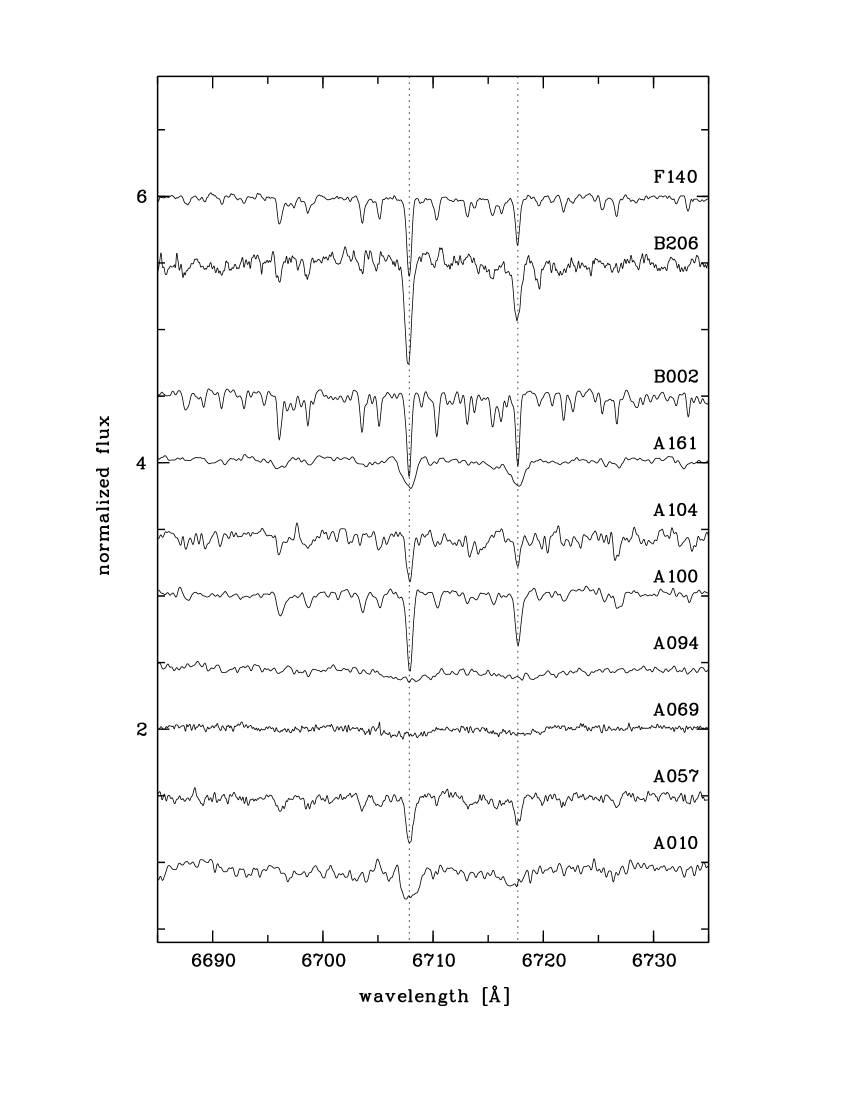
Figure 18: Spectra of the lithium-rich sample listed in Table 5. The wavelengths of Li i $\lambda 6708$ Å and Ca i $\lambda 6718$ Å are indicated by the dashed lines.

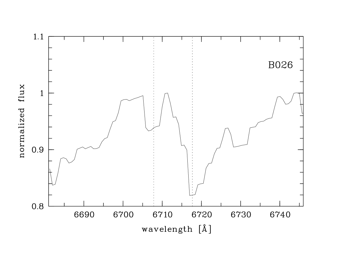
Figure 19: Low-resolution spectrum of the M4 star B026. The dashed lines indicate Li i $\lambda 6708$ Å and Ca i $\lambda 6718$ Å.

Table 5: Spectral types, lithium equivalent widths, $EW$(Li), logarithmic abundances, $\log N$(Li), and projected rotational velocities for the subsample of stars with lithium abundance above the Pleiades upper envelope. (“PMS” sample). Evolved lithium-rich stars not belonging to the PMS sample are marked by the “${\ast}$” symbol.

field	RASS name	Sp. type	$EW$(Li i )	$\log N$(Li)	$v\,\sin i$
			[mÅ]		[km s-1]
A010	RXJ0331.1$+$0713	K4Ve	407	$3.08$	$42$
A057	RXJ0344.4$-$0123	G9V-IV	277	$3.23$	$20$
A058	RXJ0344.8$+$0359	K1Ve	310	$3.17$	$31$
A069	RXJ0348.5$+$0831	G4V:	259	$3.59$	$>100$
A094	RXJ0355.2$+$0329	K3V	424	$3.39$	$>100$
A100	RXJ0358.1$-$0121	K4V	362	$2.84$	$15$
A104	RXJ0400.1$+$0818	G5V-IV	259	$3.49$	$12$
A161	RXJ0417.8$+$0011	M0Ve	304	$1.48$	$44$
B002∗	RXJ0638.9$+$6409	K3III	315	$2.17$	$6$
B026	RXJ0708.7$+$6135	M4e	272	$0.53$	$*$
B206	RXJ0828.1$+$6432	K8Ve	607	$3.06$	$16$
F140∗	RXJ2241.9$+$1431	K0III	307	$3.36$	$<5$

Table 6: Spectral types, lithium equivalent widths, $EW$(Li), logarithmic abundances, $\log N$(Li), and projected rotational velocities for the subsample of stars with lithium abundance between the Pleiades lower and upper envelope (“Pl_ZAMS” sample). Lithium-rich evolved stars not belonging to the Pl_ZAMS sample are marked by “${\ast}$”.

field	RASS name	Sp. type	$EW$(Li i )	$\log N$(Li)	$v\,\sin i$
			[mÅ]		[km s-1]
A001	RXJ0328.2$+$0409	K0	275	$3.12$	$96$
A036	RXJ0338.7$+$0136	K4Ve	80	$1.08$	$17$
A039	RXJ0338.8$+$0216	K4	58	$0.90$	$16$
A042	RXJ0339.9$+$0314	K2	104	$1.64$	$63$
A056	RXJ0343.9$+$0327	K1V-IV	126	$1.97$	$12$
A063	RXJ0347.1$-$0052	K3V	84	$1.31$	$21$
A071	RXJ0348.9$+$0110	K3V:e	258	$2.36$	$83$
A090	RXJ0354.3$+$0535	G0V	131	$3.03$	$31$
A095	RXJ0355.3$-$0143	G5V	213	$3.16$	$19$
A096	RXJ0356.8$-$0034	K3V	122	$1.55$	$22$
A101	RXJ0358.9$-$0017	K3V	294	$2.62$	$27$
A120	RXJ0404.4$+$0518	G7V	239	$3.15$	$27$
A126	RXJ0405.6$+$0341	G0V-IV	63	$2.54$	$<5$
A154	RXJ0416.2$+$0709	G0V	58	$2.50$	$11$
B008	RXJ0648.5$+$6639	G5	121	$2.58$	$9$
B018	RXJ0704.0$+$6214	K5Ve	36	$0.50$	$12$
B034∗	RXJ0714.8$+$6208	G1IV-III	127	$2.93$	$12$
B039	RXJ0717.4$+$6603	K2V	213	$2.27$	$21$
B068	RXJ0732.3$+$6441	K5e	130	$1.21$	$*$
B086∗	RXJ0742.8$+$6109	K0III	147	$1.65$	$11$
B124∗	RXJ0755.8$+$6509	G5III	153	$2.19$	$6$
B160	RXJ0809.2$+$6639	G2V	128	$2.86$	$12$
B174	RXJ0814.5$+$6256	G1V	136	$2.99$	$11$
B183	RXJ0818.3$+$5923	K0V	134	$2.21$	$7$
B185	RXJ0819.1$+$6842	K7Ve	26	$0.02$	$13$
B199	RXJ0824.5$+$6453	K4V	50	$0.83$	$26$
C047	RXJ1027.0$+$0048	G0V	73	$2.63$	$11$
C058	RXJ1028.6$-$0127	K5e	30	$0.41$	$12$
C143	RXJ1051.3$-$0734	K2V	75	$1.44$	$18$
C165	RXJ1057.1$-$0101	K4V	34	$0.65$	$7$
C176	RXJ1059.7$-$0522	K1V	148	$2.09$	$9$
C197	RXJ1104.6$-$0413	G5V	130	$2.64$	$10$
C200	RXJ1105.3$-$0735	K5e	160	$1.38$	$32$
D064	RXJ1210.6$+$3732	K0	115	$2.10$	$19$
E022	RXJ1628.4$+$7401	G1V	172	$3.21$	$18$
E067	RXJ1653.5$+$7344	G1IV	98	$2.43$	$8$
E179	RXJ1728.1$+$7239	K4IVe	66	$0.53$	$18$
F015	RXJ2156.4$+$0516	K2	185	$2.11$	$12$
F046	RXJ2212.2$+$1329	G8:V:	106	$2.23$	$5$
F060	RXJ2217.4$+$0606	K1e	108	$1.86$	$8$
F087	RXJ2226.3$+$0351	G5:V:	80	$2.31$	$31$
F101	RXJ2232.9$+$1040	K2V:	285	$2.76$	$97$
F142	RXJ2242.0$+$0946	K8V	54	$0.26$	$24$

The majority of stars has EWs and lithium abundances below the Pleiades upper limits of EW and $\log N$(Li), respectively. In the region between the upper and lower envelope of the Pleiades 43 G-K stars are found. This group is listed in Table 6. Three of these stars are giants with LC IV-III, III, and II. The 40 non-giants appear to constitute a population with an age similar to the Pleiades, i.e. $\sim$100 Myr. The region between the Hyades upper and the Pleiades lower envelope contains 23 stars of which 4 are evolved objects. The UMa age group with an age of $\sim$300 Myr thus consists of 19 stars. Below the upper limit of the Hyades 57 non-giant stars are found and are thus assigned an age of older than $\sim$600-700 Myr. Adding the 17 evolved G-K stars which are certainly also older than $\sim$1 Gyr results in a total of 74 stars for age group “Hya+”. Thus lithium abundances and luminosity classification suggest that 47% of all G-K stars in the sample have an age of less than about 600-700 Myr. Restricting these statistical considerations to the later spectral types increases the fraction of stars younger than the Hyades. Of the 114 G5-K9 stars 55, i.e. $\sim 50$%, have a lithium abundance higher than the Hyades. With the above mentioned ambiguity of the age group definition this means that at least half of the G5-K9 stars are younger than the Hyades. Some statistics of the age distribution of our sample stars for these age groups is summarized in Table 7.

5.2.3 Spatial distribution of the age groups

The spatial distribution of the G and K stars of the various age groups is summarized in Table 8. Variations of the surface density of the various age groups with location are indicated.

As expected area IV located near the north galactic pole has the lowest surface density of stars younger than the Hyades. In this area only 2 stars younger than $600-700$ Myr are found in 72 deg². This corresponds to a surface density of $0.028\pm 0.020$ deg^-2 at a RASS count-rate limit of 0.03 cts s^-1. In the other 5 areas (613.2 deg²) a total of 60 stars (including 5 stars in area V above 0.03 cts s^-1) yields a surface density of $0.0978\pm 0.013$ deg^-2. Counting stars of all age groups area IV has a surface density of $0.097\pm 0.037$ deg^-2 compared to $0.204\pm 0.018$ deg^-2 in the other areas at the same count-rate limit. A t-test shows that these differences are significant.

The very young stars of the PMS sample are apparently more abundant in area I than in any other area: 80% of these stars are found in area I. Adding up the numbers of stars younger than the Hyades in areas II, III, and VI leads to an average surface density $0.077\pm 0.013$ deg^-2. This is less than half of the value in area I which is $0.167\pm 0.034$ deg^-2 . Although indicative for a higher concentration of young stars in area I the difference is not significant.

Table 7: Statistics of the age distribution of the sample of G-K stars. “PMS” denotes stars younger than 100 Myr, “Pl_ZAMS” stars as old as the Pleiades, “UMa” stars with an age of $\sim 300$ Myr, and “Hya+” older than the Hyades. The latter age group also contains 17 evolved stars (LC IV-III, III, and II). The total number of G-K stars is 141.

	age group
	PMS	Pl_ZAMS	UMa	Hya+
	$<100$ Myr	100 Myr	$\sim 300$ Myr	$>660$ Myr
number G-K	8	40	19	74
fraction G-K	6%	28%	13%	52%

Table 8: Statistics of the spatial distribution of the various age groups in the sample. For each age group the total number of stars and the number per square degree is given. The numbers are for a RASS count-rate limit of 0.03 cts s^-1 except for area V which has a count-rate limit of 0.01 cts s^-1.

area	age group
	PMS		Pl_ZAMS		UMa		Hya+
	$<100$ Myr		100 Myr		$\sim 300$ Myr		$>660$ Myr
I	8	0.056	14	0.097	3	0.021	10	0.069
II	2	0.014	9	0.063	1	0.007	22	0.153
III	0	0	7	0.049	1	0.007	16	0.111
IV	0	0	1	0.014	1	0.014	5	0.069
V	0	0	3	0.084	6	0.161	11	0.296
VI	0	0	6	0.042	7	0.049	10	0.069

5.2.4 Age dependent $\log N-\log S$ distribution

We compared the observed cumulative number distribution, $\log N(>S)-\log S$, of our sample with model predictions by Guillout et al. (Guilloutetal96 (1996)). The median latitude for the combined areas I, II, III, V, and VI, which are distributed between galactic latitudes of 20$\degr$ and 50$\degr$, is actually $30\degr$, thus matching this model parameter well. The models of Guillout et al. (Guilloutetal96 (1996)) give cumulative surface densities, $N(>S)$, as a function of ROSAT-PSPC count rate, $S$, for three age bins: age younger then 150 Myr, age between 150 Myr and 1 Gyr, and older than 1 Gyr. We restricted the comparison to the youngest model age bin and to the sum of all model age bins because of the difficulty to separate observationally stars with ages of several 100 Myr to $\sim 1$ Gyr and older. We further considered the combined sample of G and K stars. M stars were not included because of the lack of an observational age determination for stars of this spectral type in our sample. The uncertainty of the ages derived observationally from lithium was taken into account by forming two observational age samples matching as closely as possible the youngest age bin of the models: a) a sample comprising the sum of G-K stars from the PMS and Pl_ZAMS age group, and b) a sample containing in addition the corresponding UMa stars. The true sample of stars younger than 150 Myr is expected to lie between these limits.

The result of the comparison of $\log N(>S)-\log S$ is depicted in Fig. 20 for three RASS X-ray count rates of 0.1, 0.3 and 0.01 cts s^-1. The predicted numbers of G-K are in good agreement with our sample in the 5 study areas located around $30\degr$ in galactic latitude. This holds for both the sum of all age groups and stars younger than $\sim 150$ Myr obtained as described above and represented in the figure by the filled symbols. Likewise, the predicted flattening of $\log N(>S)-\log S$ at lower count rates is also found in our data for area V which has the lowest count rate limit of 0.01 cts s^-1.

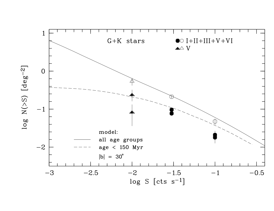
Figure 20: Comparison of observed co-added number densities of G and K stars, $N(>S)$, for three RASS count rates $S$ with models of Guillout et al. (Guilloutetal96 (1996)) for $|b|=30\degr$. Open symbols denote the sum of all age groups. Lower and upper filled symbols represent the sum of age groups “PMS” and “Pl_ZAMS”, and of “PMS”, “Pl_ZAMS”, and UMa, respectively.

5.3 Kinematics

5.3.1 Proper motions

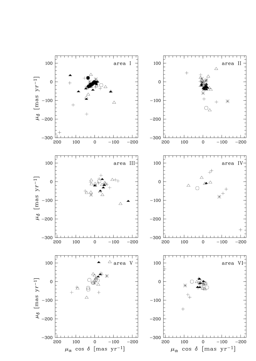
Figure 21: Proper motions for the six study areas. The different symbols denote the different age groups: filled circles = PMS, filled triangles = Pl_ZAMS, open circles = UMa, open triangles = Hya+, $\ast$ = giants, $+$ = M stars without Li detection.

We searched for proper motions in a variety of different catalogs: the Hipparcos Catalog (ESA Hipparcos (1987)), the Positions and Proper Motions Catalog (PPM) (Röser & Bastian PPM (1988)), the ACT Reference Catalog (Urban et al. ACT (1997)), the Tycho Reference Catalogue (TRC) (Hog et al. Hogetal98 (1998)), the Tycho-2 catalog (Hog et al. Hogetal00 (2000)), the STARNET catalog (Röser STARNET (1996)), and the Second U.S. Naval Observatory CCD Astrograph Catalog (UCAC2) (Zacharias et al. UCAC2 (2003)). The PPM and the STARNET catalogs were locally transformed to the Hipparcos reference system before identification. For many stars we found entries in more than one catalog, and in these cases the proper motions were compared and the one which had consistent solutions across several catalogs was usually chosen. If all proper motions were consistent, the most precise one was adopted; this was usually the Hipparcos or the UCAC2 proper motion (the Hipparcos catalog has a high weight in the solution for the UCAC2 proper motion), or the Tycho-2 proper motion for those regions not covered yet by the UCAC2 catalog. However, in many cases the proper motion in Hipparcos differed from the entries in other catalogs, which is likely due to the fact that the Hipparcos proper motions reflect the ’instantaneous’ motion during the Hipparcos mission, which is often affected by orbital motion, whereas most of the proper motions in the other catalogs are based on observations stretched out over a longer baseline and thus better reflect the real motion of the center of mass through space which is of interest here.

Altogether, we were able to assign proper motions to the counterparts of 129 RASS sources with spectral types G to M. In detail we found 55 of 56 G stars, 61 of 86 K stars and 13 of 56 M stars in the mentioned catalogs. In addition we also found 54 F stars. An equal number of proper motions comes from Tycho-2 and UCAC2, while only two proper motions each were taken from Hipparcos and TRC, and only one each from PPM and STARNET, while the ACT was not used in the end at all.

These proper motion data were supplemented for the optically faint stars (mainly of spectral type K and M) by data from other catalogs: 53 stars from USNO-B1.0 (Monet et al. USNOB1 (2003), 36 M stars, 16 K stars, and 1 G star), 1 M star from Carlsberg Meridian Catalogs (Carlsberg (1999)), and 1 M star from the NPM1 Catalog of the Lick Northern Proper Motion Program (Klemola et al. Klemolaetal87 (1987)). Note that the USNO-B1.0 proper motions are not absolute, but relative to the Yellow Sky Catalog YS4.0 in the sense that the mean motion of objects common to USNO-B1.0 and YS4.0 was set to zero in USNO-B1.0. According to Monet et al. (USNOB1 (2003)) the difference between these relative proper motions and the true absolute ones should, however, be small.

Thus in total proper motion data are available for all G stars, for 77 of 86 K stars, and for 51 of 56 M stars.

The proper motions are shown in Fig. 21 for the individual study areas. The diagram displays proper motions for six groups of stars, i.e. the “PMS” ”Pl_ZAMS”, “UMa” and “Hya+” age groups, evolved stars (giants) and the M stars without lithium detection.

Of particular interest are the proper motions of the stars of the youngest age groups in area I, i.e. the “Pl_ZAMS” and “PMS” samples with ages of 100 Myr and less, This study area is located near the Tau-Aur SFR and near the Gould Belt (see Fig. 1) and has, probably due to its location, the highest surface density of young stars. Proper motions exist for all eight young stars of area I listed in Table 5. They are plotted in the upper left panel of Fig. 21. Four of the stars of age group PMS in area I were already identified as pre-main sequence objects by Neuhäuser et al. (Neuhaeuseretal97 (1995)) (A058, A069, A090, and A104). They assigned an age of 35 Myr to these stars. Likewise, one star of the Pl_ZAMS sample, A120, was assigned an age of 100 Myr by Neuhäuser et al.. These stars were part of a sample investigated kinematically for membership to the Taurus-Auriga SFR by Frink et al. (Frinketal97 (1997)). They studied stars in the central region of Tau-Aur and in a region south of Tau-Aur which partially overlaps at the southern edge with our area I. The sample studied by these authors contains three further stars of our sample, A007, A107, and A122, for which Neuhäuser et al. assigned an age of older than 100 Myr. This is in agreement with our age estimate of older than 660 Myr for A007 and A107, and of $\sim$300 Myr for A122.

In Table 9 the mean proper motions and their dispersions are summarized for the PMS, Pl_ZAMS, UMa, and Hya+ age groups, and for M stars without Li i  detection. Obviously, the 8 “PMS” stars show a smaller spread in proper motions than the older stars. They cluster around ($\mu_{\alpha}\cdot\cos\delta$, $\mu_{\delta}$) of ($+16,-8$) mas yr^-1 with a scatter of $\sim 15$ mas yr^-1 in each direction. Frink (Frink99 (1999)) transformed the proper motions given by Frink et al. (Frinketal97 (1997)) from the FK5 to the Hipparcos system and determined mean values of ($+8.7,-11.2$) mas yr^-1 for the southern sample of Frink et al. (Frinketal97 (1997)). For the central region of Tau-Aur Frink (Frink99 (1999)) derived mean proper motions of ($+4.5,-19.7$) mas yr^-1. The comparison of our results with the findings of Frink (Frink99 (1999)) reveals an interesting trend in the mean proper motions relative to the core region of Tau-Aur. The southern sample of Frink et al. moves away from the centre of Tau-Aur with a mean proper motion of (+4.2,+8.5) mas yr^-1. The PMS stars in area I are located even more to the south of the centre and their relative mean proper motion is actually even larger, (+12,+12) mas yr^-1. Thus we find that the stars in area I move in approximately the same direction as the southern stars of Frink et al., but with an even higher proper motion.

Inspection of Fig. 2 in Frink et al. (Frinketal97 (1997)) allows to estimate a dispersion of about 15 to 20 mas yr^-1 for both subsamples which again is compatible with the 15 mas yr^-1 derived for our PMS subsample. The Pl_ZAMS stars exhibit a dispersion of the proper motion which is larger by a factor of 2 to 3. On the other hand, the UMa sample though being older shows more coherent proper motions with a dispersion equal to the PMS stars. The old stars of the Hya+ group and the M stars exhibit the largest dispersions. Similar results are found for the other study areas.

Table 9: Mean proper motions and dispersions in area I for stars of age groups PMS, Pl_ZAMS, UMa, and M stars without lithium detection (in mas yr^-1).

age group	$\langle\mu_{\alpha}\cos\delta\rangle$	$\sigma_{\alpha}$	$\langle\mu_{\delta}\rangle$	$\sigma_{\delta}$
PMS	$+16$	15	$-8$	14
Pl_ZAMS	$+18$	52	$-22$	32
UMa	$+16$	15	$-8$	14
Hya+	$-33$	69	$-42$	55
M stars	$+59$	64	$-67$	131

So far we have considered the proper motions which depend on the distance and contain a contribution due to the solar motion. We therefore calculated tangential velocity components, $v_{l}$ and $v_{b}$, in galactic coordinates, $l$ and $b$, by using the distance estimates discussed above and the relations $v_{l}=4.74\times\mu_{l}\,\cos\,b\times d$ km s^-1 and $v_{b}=4.74\times\mu_{b}\times d$ km s^-1, with $\mu_{l}\,\cos\,b$ and $\mu_{b}$ being proper motions in galactic coordinates given in arcsec yr^-1 and the distance $d$ in pc. A table summarizing the resulting velocities and their dispersions for the individual study areas can be found in the Appendix (Table 12).

The direction-dependent part of the tangential velocities due to the solar reflex motion can finally be removed by transforming these velocities to the local standard of rest (LSR). This is achieved by adding the corresponding solar velocity components. We used the solar motion vector of Dehnen & Binney (DehnenBinney98 (1998)), ($U_{\sun}$, $V_{\sun}$, $W_{\sun}$) = (+10.0, +5.25, +7.17) km s^-1 (see below for the definition of the space velocities) to determine the solar reflex motion:

$$v_{l,\sun}=-U_{\sun}\sin l+V_{\sun}\cos l$$ (1)

$$v_{b,\sun}=U_{\sun}\cos l\sin b-V_{\sun}\sin l\sin b+W_{\sun}\cos b$$ (2)

In contrast to the observed proper motions the tangential velocity components of the different object groups exhibit a similar scatter around the mean of the respective sample. This is particularly evident for the M stars which have on average the smallest distances and hence have the largest proper motions. Generally, the dispersions of their tangential velocities are of the same order of magnitude as for the other object groups, although there are some differences between the individual study areas. From the kinematical point of view the M stars in area I appear to be young, $\sim 100$ Myr, as they resemble the Pl_ZAMS group with regard to both the mean velocity and the velocity dispersion. This also holds for area III and VI where the M stars kinematically appear somewhat older, $\sim 300$ Myr, with velocity dispersions between the Pl_ZAMS and the Hya+ group. In area II, IV, and V, on the other hand, the M stars show kinematical resemblance to the Hya+ age group suggesting an age of $\ga 600$ Myr.

In Table 10 mean proper motions in galactic coordinates with respect to the LSR, $\langle\mu_{l}\cos b\rangle_{\rm LSR}$ and $\langle\mu_{b}\rangle_{\rm LSR}$, and the corresponding tangential velocities, $\langle v_{l}\rangle_{\rm LSR}$ and $\langle v_{b}\rangle_{\rm LSR}$ are listed for the different age groups. As discussed before the M stars exhibit the largest dispersion of the proper motions. Taking the distance effect into account the dispersions of the respective tangential velocities are reduced to values similar to those obtained for the Pl_ZAMS and UMa age groups. This again leads to the conclusion that the M stars have on the average an age of $\sim$100-600 Myr. The largest velocity dispersions are found for the Hya+ age group.

Table 10: Mean proper motions (in mas s^-1), and mean tangential velocities (in km s^-1) in galactic coordinates, both with dispersions, reduced to the LSR. The values are listed for stars of the age groups PMS, Pl_ZAMS, UMa and Hya+ (split into dwarfs and giants), and M stars without lithium detection.

age group	$\langle\mu_{l}\ cosb\rangle_{\rm LSR}$	$\langle\mu_{b}\rangle_{\rm LSR}$	$\langle v_{l}\rangle_{\rm LSR}$	$\langle v_{b}\rangle_{\rm LSR}$
PMS	$+3\pm 14$	$+11\pm 17$	$+0\pm 8$	$+14\pm 11$
Pl_ZAMS	$+8\pm 29$	$+2\pm 35$	$+2\pm 18$	$+5\pm 14$
UMa	$-8\pm 37$	$+0\pm 27$	$-14\pm 36$	$+0\pm 15$
Hya+:
dwarfs	$-7\pm 75$	$-7\pm 42$	$-47\pm 310$	$-26\pm 184$
giants	$+21\pm 39$	$-5\pm 31$	$+5\pm 72$	$+4\pm 34$
M stars	$+22\pm 108$	$-34\pm 139$	$-5\pm 20$	$-2\pm 23$

5.3.2 Space velocities

For stars with a distance estimate from trigonometric, spectroscopic or IR photometric parallax radial velocities and proper motions were combined in order to determine the galactic space velocity components $U$, $V$, and $W$. A right-handed coordinate system was used with the $U$ axis pointing towards the galactic centre, the $V$ axis in the direction of galactic rotation, and the $W$ axis towards the north galactic pole. The transformation to the LSR was performed by using the solar motion vector of Dehnen & Binney (DehnenBinney98 (1998)) given above. The required data, RVs, proper motions, and distances, were available for 44 of 56 G stars, 46 of 85 K stars, and 7 of 56 M stars. The space velocity components and related errors were calculated using the formulae given by Johnson & Soderblom (JohnsonSoderblom87 (1987)). For the calculation of the errors an uncertainty of 50% was adopted for the distance for stars with a spectroscopic or photometric parallax. The resulting velocity components are listed in Table 14.

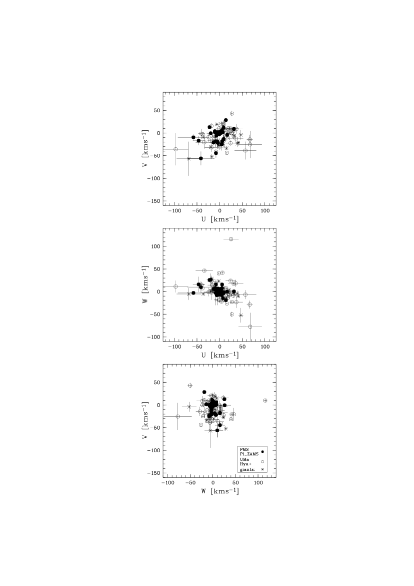
Figure 22: Space velocities $U$, $V$, and $W$ in the LSR frame. Stars of age groups “PMS” and “Pl_ZAMS” are plotted as filled circles. Open circles denote stars of the UMa and “Hya+” age group. Giants are plotted as asterisks.

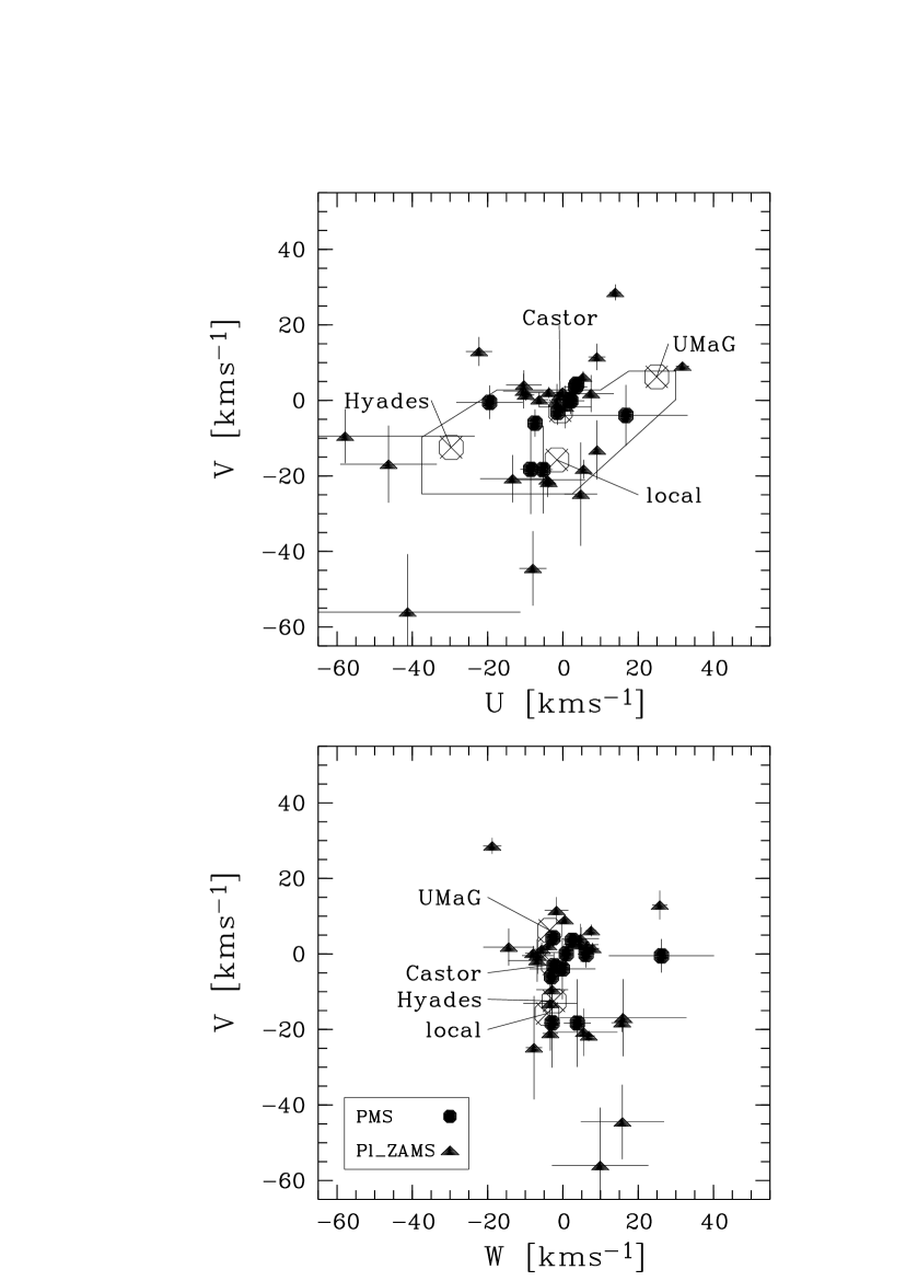
Figure 23: Upper panel: $U-V$ velocity diagram for the youngest age groups “PMS” (circles) and “Pl_ZAMS” (triangles). The solid line encircles the region defined by Eggen (Eggen84 (1984), Eggen89 (1989)) to contain the young disk population. Also shown as large crossed circles are the $U$ and $V$ velocities of the Hyades supercluster, the Local Association (designated “local”), the Castor MG, and the UMa MG. Lower panel: $W-V$ diagram for the same sample of stars. All velocities are in the LSR reference frame.

Table 11: Mean (M-L) space velocity components, $\langle U\rangle,\langle V\rangle,\langle W\rangle$, and velocity dispersions, $\sigma_{U}$, $\sigma_{V}$, $\sigma_{W}$, of the different age groups in km s^-1.

	$\langle U\rangle$	$\sigma_{U}$	$\langle V\rangle$	$\sigma_{V}$	$\langle W\rangle$	$\sigma_{W}$
PMS	$-1.9\pm 2.6$	$4.2\pm 3.1$	$+0.2\pm 2.2$	$2.9\pm 2.5$	$+0.0\pm 1.7$	$2.4\pm 2.1$
Pl_ZAMS	$-1.5\pm 4.1$	$11.9\pm 3.8$	$-4.4\pm 4.8$	$14.6\pm 4.6$	$+1.1\pm 3.2$	$9.3\pm 2.9$
UMa	$+18.2\pm 6.6$	$12.1\pm 11.1$	$-1.2\pm 10.8$	$22.1\pm 10.6$	$-5.2\pm 10.5$	$21.8\pm 10.1$
Hya+:
dwarfs	$+5.5\pm 7.0$	$22.4\pm 6.6$	$-7.9\pm 5.3$	$16.3\pm 4.6$	$+6.4\pm 8.8$	$29.2\pm 7.8$
giants	$+4.5\pm 11.7$	$28.4\pm 12.9$	$-15.0\pm 8.9$	$19.2\pm 8.1$	$+0.3\pm 5.8$	$13.4\pm 6.2$

The space velocities components are plotted in Fig. 22. The plot contains stars of all age groups and also includes the evolved stars (giants). Figure 23 shows in an enlarged scale the $V-U$, and $V-W$ diagrams for the two youngest stellar age groups only, i.e. PMS and Pl_ZAMS stars.

As can be seen in Fig. 22 the filled symbols representing the youngest age groups, PMS and Pl_ZAMS, are more concentrated than the open symbols and the asterisks denoting the older age groups and giants, respectively. This can be tested by various statistical methods. First, we combined on one hand the PMS and Pl_ZAMS samples and on the other hand the older stars and giants in order to create distributions of the space velocity $v_{\rm LSR}=\sqrt{U^{2}+V^{2}+W^{2}}$ for the young and the old stars, respectively. A one-dimensional two-sample Kolmogorov-Smirnov (K-S) test on these distributions yields a probability of $<1.6\,10^{-5}$ that they are drawn from the same parent distribution. Likewise, the K-S test on the PMS and the complementary non-PMS sample yields a probability of only $5\,10^{-4}$ for having the same distribution. Therefore, PMS and non-PMS stars also have different space velocity distributions. Contrary to this, with a probability of 0.31 PMS and Pl_ZAMS stars have the same distribution. An F-test on the individual velocity components $U$, $V$, and $W$ of the combined PMS-Pl_ZAMS and the older age groups shows that with a very low probability $P$ their distributions are drawn from the same parent distribution, namely $P_{U}=0.006$, $P_{V}=0.02$, and $P_{W}=4\,10^{-6}$. In particular, the velocity component perpendicular to the galactic plane, $W$, is significantly different in the young and the old age groups (see below).

In the following we will discuss mean velocities and velocity dispersions of the different age groups. These were calculated as maximum-likelihood (M-L) estimate which takes into account that the measurement errors are different for each star. Following Pryor & Meylan (PryorMeylan93 (1993)) M-L estimates of the mean velocity components $\langle v\rangle$ and dispersions $\sigma_{v}$ of $U,V$ and $W$ were obtained together with errors by assuming that the velocities are drawn from a normal distribution

$$f(v_{i})=\frac{1}{\sqrt{2\,\pi(\sigma_{v}^{2}+\sigma_{i}^{2}})}\exp\left(-\frac{1}{2}\frac{(v_{i}-\langle v\rangle)^{2}}{(\sigma_{v}^{2}+\sigma_{i}^{2})}\right)$$ (3)

with the individual velocity measurements $v_{i}$ and associated errors $\sigma_{i}$ of $U,V,$, and, $W$, respectively. With the likelihood function $\cal L$ defined as

$${\cal L}=\prod_{i=1}^{n}f(v_{i})$$ (4)

the minimization of the test statistic $S=-2\,\ln{\cal L}$ then allows to derive the M-L estimates of $\langle v\rangle$ and $\sigma_{v}$. Errors were calculated following Pryor & Meylan.

In Table 11 the mean space velocities and velocity dispersions of the different age groups are summarized. Clearly the PMS sample has the smallest velocity dispersions. For stars with weak or no lithium detection the dispersions are the largest. The “Hya+” subsample contains a significant fraction of older disk stars. This is particularly evident for the velocity component perpendicular to the galactic plane, $W$. Its dispersion increases from $\sim 2$ km s^-1 for the PMS sample to $\sim 30$ km s^-1 for the old lithium weak sample. The increasing velocity dispersion with increasing age reflects the effect of disk heating in the galaxy.

The PMS subsample in particular exhibits M-L mean space velocity components $(\langle U\rangle,\langle V\rangle,\langle W\rangle)=(-1.9\pm 2.6,+0.2\pm 2.2,+0.0\pm 1.7)$ km s^-1 and velocity dispersions of ($\sigma_{U},\sigma_{V},\sigma_{W})=(4.2\pm 3.1,2.9\pm 2.5,2.4\pm 2.1$) km s^-1. This suggests that the PMS stars are kinematically related and may even form a kinematical group, but of course, the sample is small and the indicated relation should be considered more as a working hypothesis to be tested with extended samples. At this point it should be noted that the PMS star B206 in area II interestingly has space velocity components similar to the stars in area I. Unfortunately, no high resolution RV measurement is available for the second PMS star in area II, the M4Ve dwarf B026. In order to obtain at least an estimate of its space velocity components we measured the radial velocity using the low-resolution CAFOS spectra and the emission lines of H$\alpha$, H$\beta$, H$\gamma$, and Ca ii K. This yielded $v_{\rm hel}=-12$ km s^-1  with an error of about 20 km s^-1. The resulting space velocity components are $U=+20\pm 17$ km s^-1, $V=+1\pm 8$ km s^-1, and $W=+2\pm 9$ km s^-1. Within the errors the velocities of B026 are consistent with the mean velocities of the PMS sample. But clearly, a more accurate RV measurement is needed for B026 to confirm that both Li-rich stars in area II belong to the same kinematical group as the corresponding stars in area I as indicated by the presently available data. Note also from Fig. 24 that in areas I and II the numbers of Li-rich stars are higher than in the other areas.

Enlarged sections of the $U-V$ and $W-V$ diagram are shown in Fig. 23 for the 35 stars of the two youngest age groups with measured space velocities. The $U-V$ diagram in the upper panel includes the limits of the region occupied by the young disk stars as defined by Eggen (Eggen84 (1984), Eggen89 (1989)). Indeed, as expected for a young stellar sample many, albeit not all, stars have $(U,V)$ velocities inside Eggen’s box. Also indicated are the $(U,V)$ velocities of several young stellar kinematical groups: the Hyades supercluster, the Ursa Major moving group (UMa MG), the Local Association (Pleiades MG), and the Castor moving group (Castor MG) (for references see e.g. Montes et al. Montesetal01 (2001)).

Figure 23 suggests the existence of a kinematical subgroup in the combined PMS and Pl_ZAMS sample, which contains 35 stars with measured $U$, $V$, and $W$ velocities. The group is concentrated near the velocity of the Castor MG at the upper $V$ limit of Eggen’s disk stars with 17 of the 35 stars found within a radius of 10 km s^-1 around the velocity of the Castor MG. Six of these belong to the age group PMS and the rest to the Pl_ZAMS group. The M-L mean velocities of the subgroup are $(U,V)=(-1.4\pm 1.7,+2.3\pm 0.9)$ km s^-1, and the velocity dispersions are $(\sigma_{U},\sigma_{V})=(4.3\pm 1.0,1.2\pm 0.6)$ km s^-1. In $V$ the group of 17 stars is somewhat off the Castor MG for which Palouš & Piskunov (PalousPiskunov85 (1985)) give ($U,V)=(-0.7\pm 3.5,-2.8\pm 2.4)$ km s^-1. Given the relatively small number of data points we may ask whether this concentration is due to a chance coincidence in an actually random distribution. We tested this possibility for the null hypothesis that the true underlying distribution of velocities in the $U-V$ plane is random within a given circle around the origin. In a Monte Carlo simulation we calculated a large number of random velocity vectors in the $U-V$ plane and counted the number of cases in which we found 17 stars within 10 km s^-1 around the Castor MG velocity. For a random velocity distribution within a radius of $35$ km s^-1 containing 90% of the 35 stars, i.e. 31 stars, these simulations showed that we can reject the null hypothesis on a high significance level of $>99.8$%. The test radius of $35$ km s^-1 may be too small because it excludes 10% of the stars. Increasing the radius leads however to even higher significance levels. Decreasing the radius only leads to significance levels of $<99$% if the random distribution is calculated for radii smaller than $\sim$20 km s^-1 which contains $\leq$65% of the PMS-Pl_ZAMS stars. Therefore we are lead to the conclusion that with a very high probability the concentration of velocities vectors in the $U-V$ plane is not a chance coincidence.

An interesting feature is the accumulation of the 6 “PMS” stars around a mean velocity of ($U,V)=(+0.0\pm 2.9,+1.2\pm 2.8)$ km s^-1. This is not far from the velocity of the Castor MG (see above), but clearly distinct from the Local Association which has ($U,V)=(-1.6,-15.8)$ km s^-1 (Montes et al. Montesetal01 (2001)). The velocity dispersions of this subgroup of PMS stars are $(\sigma_{U},\sigma_{V})=(3.5\pm 1.7,2.5\pm 2.1)$ km s^-1. Two of the remaining PMS stars are found near the velocity of the Local Association together with a loose accumulation of some 5 or 6 further stars from the Pl_ZAMS age group. A relation of these stars with the Local Association may exist, but the errors and the scatter of the velocity vectors are quite large.

The $W-V$ diagram displayed in the lower panel of Fig. 23 shows a similar trend in the distribution of the velocity vectors as in the $U-V$ diagram, that is most PMS stars and many Pl_ZAMS stars are kinematically distinct from the Local Association.

6 Conclusions

We have investigated the characteristics of an X-ray selected sample from the RASS of high-galactic latitude field stars comprising 56 G, 86 K, and 56 M type stars. Spectroscopic low/medium and high resolution follow-up observations were obtained for 95% of the G-K stars and for 77% of the M stars.

Spectroscopic luminosity classification of the G-K stars based on the high resolution spectroscopy showed that 88% of the G-K stars are main-sequence stars or subgiants of luminosity classes V and IV, respectively. From IR photometric classification we concluded that all M stars are dwarf stars.

Significant lithium absorption lines were detected in a large fraction of stars with equivalent widths and abundances, respectively, above the level of the Hyades in about 50% of the stars. For the age distribution of the high-galactic latitude coronal sample this means that about half of the G-K stars are younger than the Hyades. About 25% of the G-K stars have an age comparable to that of the Pleiades, i.e. $\sim 100$ Myr. A small fraction of less than 10% of the G-K stars is younger than the Pleiades. Most PMS stars, i.e. 8 out of 10, are located in area I. Only two PMS stars are found in area II and none in the remaining areas. This suggests a possible relation of the high-$|b|$ PMS stars to the Gould Belt indicated in Fig. 1. However, the subsample formed by combining the stellar age groups PMS and Pl_ZAMS is spatially distributed in all directions covered by our study areas. At the same time half of its members show similar kinematical parameters independent of spatial location. This questions the relation to the Gould Belt. Rather, the space velocities suggest that these stars are members of a loose moving group with a mean velocity close to that of the Castor MG. For the Castor MG an age of 200$\pm$100 Myr has been derived by Barrado y Navascués (Barrado98 (1998)). This would still be consistent with the Pl_ZAMS group. If some of the PMS stars are indeed kinematically related to the Castor MG this would indicate a large age spread in this moving group as they appear to be younger than 100 Myr, maybe even as young as $\sim 30$ Myr.

Appendix A Parameters of the sample and results

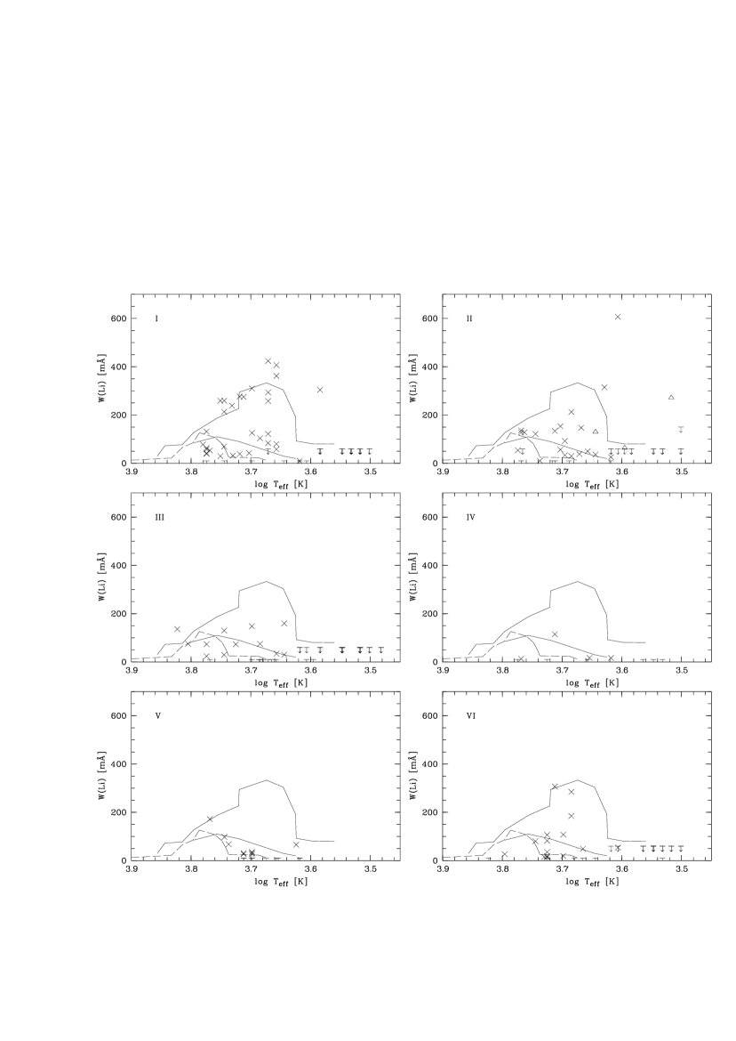
Figure 24: Equivalent widths of Li i $\lambda 6708$ as a function of $T_{\rm eff}$ plotted for each study area individually. The solid and dashed lines have the same meaning as in Fig. 16.

Figure 24 displays the measured lithium equivalent widths for each study area separately.

Table 12 summarizes for the individual study areas the mean tangential velocities in galactic coordinates, $v_{l}$ and $v_{b}$, and their dispersions as calculated in Sect. 5.3.1. The mean solar velocity components, $\langle v_{l,\sun}\rangle$ and $\langle v_{b,\sun}\rangle$, are also given for each study area. Furthermore, for each age group mean distances $\langle d\rangle$ are given.

Table 12: Mean tangential velocities and dispersions (in km s^-1) in galactic coordinates for stars of age groups PMS, Pl_ZAMS, UMa, Hya+ (split into dwarfs and giants), and M stars without lithium detection for the individual study areas. The first two lines give the average solar velocity for each study area. The mean distance $\langle d\rangle$ and its scatter are given in pc. The number of stars used for the calculation of the mean values are given in parentheses.

area	I	II	III	IV	V	VI
$\langle v_{l,\sun}\rangle$	$-4$	$-9$	$+8$	$-5$	$-11$	$-8$
$\langle v_{b,\sun}\rangle$	$-0$	$+10$	$+11$	$+10$	$+4$	$+11$
PMS:
$\langle v_{l}\rangle$	$+9\pm 9(8)$	$+7\pm 2$ (2)	–	–	–	–
$\langle v_{b}\rangle$	$+5\pm 11$ (8)	$-3\pm 1$ (2)	–	–	–	–
$\langle d\rangle$	$121\pm 53$ (8)	$51\pm 20$ (2)	–	–	–	–
Pl_ZAMS:
$\langle v_{l}\rangle$	$+11\pm 13$ (13)	$+13\pm 4$ (8)	$-6\pm 8$ (6)	–	$+52\pm 26$ (3)	$+2\pm 4$ (6)
$\langle v_{b}\rangle$	$-1\pm 15$ (13)	$-5\pm 7$ (8)	$-19\pm 11$ (6)	–	$+7\pm 19$ (3)	$-6\pm 12$ (6)
$\langle d\rangle$	$118\pm 56$ (14)	$117\pm 50$ (9)	$91\pm 39$ (7)	–	$226\pm 191$ (3)	$101\pm 77$ (6)
UMa:
$\langle v_{l}\rangle$	$+4\pm 13$ (2)	–	–		$-24\pm 42$ (6)	$-10\pm 18$ (6)
$\langle v_{b}\rangle$	$-10\pm 12$ (2)	–	–		$-10\pm 21$ (6)	$-7\pm 8$ (6)
$\langle d\rangle$	$323\pm 191$ (3)	–	–		$332\pm 252$ (6)	$240\pm 184$ (6)
Hya+:
dwarfs:
$\langle v_{l}\rangle$	$+3\pm 12$ (8)	$+4\pm 17$ (6)	$-6\pm 39$ (9)	$+11\pm 23$ (4)	$+12\pm 15$ (3)	$-11\pm 45$ (4)
$\langle v_{b}\rangle$	$-5\pm 15$ (8)	$-9\pm 9$ (6)	$-15\pm 16$ (9)	$-2\pm 26$ (4)	$-3\pm 8$ (3)	$-24\pm 36$ (4)
$\langle d\rangle$	$82\pm 46$ (8)	$132\pm 165$ (6)	$90\pm 56$ (9)	$204\pm 102$ (4)	$56\pm 45$ (3)	$201\pm 245$ (4)
giants:
$\langle v_{l}\rangle$	$-2\pm 12$ (2)	$+11\pm 93$ (10)	–	–	$+6\pm 21$ (2)	–
$\langle v_{b}\rangle$	$+7\pm 7$ (2)	$-8\pm 42$ (10)	–	–	$+15\pm 19$ (2)	–
$\langle d\rangle$	$124\pm 26$ (2)	$601\pm 810$ (10)	–	–	$175\pm 101$ (2)	–
M stars:
$\langle v_{l}\rangle$	$+12\pm 10$ (12)	$0\pm 21$ (5)	$-8\pm 16$ (10)	$-3\pm 27$ (6)	$+6\pm 27$ (8)	$+10\pm 18$ (7)
$\langle v_{b}\rangle$	$+0\pm 9$ (12)	$+5\pm 16$ (5)	$-15\pm 15$ (10)	$-44\pm 35$ (6)	$-10\pm 27$ (8)	$-19\pm 11$ (7)
$\langle d\rangle$	$43\pm 30$ (14)	$60\pm 24$ (6)	$56\pm 32$ (11)	$53\pm 27$ (6)	$59\pm 23$ (8)	$43\pm 15$ (7)

The following Tables 13 to 15 are available as Online Material only.

In Table 13 the basic parameters of the stellar sample are listed. The field and RASS names were taken from Paper III. Coordinates R.A. (2000) and DEC. (2000) of the optical counterparts are in succession either from Tycho-2, GSC-I, or GSC-II, whatever the source is for the $V$ magnitude listed in column “V”. In column “Sp.type” the revised spectral types with luminosity class are given for objects with new high resolution observations. Otherwise, spectral types from Paper III are given. Spectroscopic binaries are flagged by “SB2”. B160 is a triple system (SB3). The flux ratio $\log f_{\rm x}/f_{V}$ is given for the revised V magnitudes and the RASS fluxes from Paper III. X-ray luminosities $L_{\rm x}$ were calculated using the distances listed in column “dist”. The distances are flagged by “S”, “H”, “T” or “I”, depending on whether they were derived from spectroscopy, Hipparcos, trigonometric parallaxes, or from the infrared colours, respectively. Distance estimates obtained by assuming luminosity class V are flagged by “M”. They should be considered as lower limits only.

Table 14 lists the kinematical parameters. Heliocentric radial velocities and errors for single stars and for the primary component of spectroscopic binaries are given in columns $v_{\rm hel,1}$ and $\sigma_{1}$, respectively. For binaries columns $v_{\rm hel,2}$ and $\sigma_{2}$ contain the heliocentric radial velocity and error of the secondary component, respectively. Proper motions and associated errors are listed in columns $\mu_{\alpha}\,\cos\delta$ and $\sigma_{\mu_{\alpha}}$ for right ascension, and $\mu_{\delta}$ and $\sigma_{\mu_{\delta}}$ for declination, respectively. The source catalog of the proper motions is denoted by respective flags: TY = Tycho-2, HI = Hipparcos, UC = UCAC2, US = USNO-B1.0, PP = PPM, ST = STARNET, TR = TRC, NL = NLPM1, CA = Carlsberg Meridian Catalogs. Also given are the galactic velocity components $U$, $V$, and $W$ in the LSR frame with errors $\sigma_{U},\sigma_{V},$ and $\sigma_{W}$, respectively. If the errors were larger than 30 km s^-1 the space velocity components were omitted.

Table 15 lists lithium data and rotational velocities. Equivalent widths of Li i  $\lambda 6708$ are listed in column $W($Li i ). Flags “h”, “l”or “m” denote high-, low- or medium resolution measurements, respectively. Lithium abundances derived from $W($Li i ) for the effective temperatures given in column $T_{\rm eff}$ are listed in column $\log N$(Li). The last two columns list the rotational velocities, $v_{\rm rot_{1}}$ for single stars or primary components of binaries, and in the latter case $v_{\rm rot_{2}}$ for the secondary component.

Table 13: Basic optical and X-ray parameters of the sample of G-, K-, and M-type stars.

field	RASS name	R.A.	DEC.	Sp. type		$V$	$\log f_{\rm x}/f_{V}$	dist.		$\log L_{\rm X}$
		(2000)	(2000)					[pc]		[erg s-1]
A001	RXJ0328.2$+$0409	03:28:14.9	$+$04:09:48	K0	SB2	9.63	$-2.08$	76:	M	30.23
A007	RXJ0330.7$+$0305	03:30:43.5	$+$03:05:48	K1	SB2	10.80	$-2.62$	119:	M	29.62
A010	RXJ0331.1$+$0713	03:31:08.4	$+$07:13:25	K4Ve		10.86	$-2.07$	62	S	29.88
A013	RXJ0331.4$+$0455	03:31:25.7	$+$04:55:08	M4e		13.50	$-1.53$	28	I	28.67
A028	RXJ0336.5$+$0726	03:36:34.3	$+$07:26:20	G9V		10.89	$-2.56$	105	S	29.83
A030	RXJ0336.6$+$0329	03:36:40.7	$+$03:29:22	M5Ve		13.86	$-1.62$	14	T	27.86
A035	RXJ0337.9$-$0230	03:37:53.8	$-$02:30:12	M0e		*	$*$	*		*
A036	RXJ0338.7$+$0136	03:38:44.5	$+$01:36:50	K4Ve		13.27	$-1.76$	189	S	30.20
A039	RXJ0338.8$+$0216	03:38:48.8	$+$02:16:28	K4	SB2	9.48	$-2.70$	47:	M	29.25
A042	RXJ0339.9$+$0314	03:39:59.1	$+$03:14:31	K2	SB2	12.07	$-2.46$	194:	M	29.69
A045	RXJ0341.4$-$0013	03:41:22.8	$-$00:13:25	K3		*	$*$	*		*
A050	RXJ0342.6$+$0606	03:42:42.0	$+$06:06:36	M4e		15.58	$-0.61$	73	I	29.60
A056	RXJ0343.9$+$0327	03:43:54.3	$+$03:26:47	K1V-IV		8.96	$-3.68$	73	S	29.18
A057	RXJ0344.4$-$0123	03:44:26.0	$-$01:23:32	G9V-IV		10.19	$-2.17$	141	S	30.76
A058	RXJ0344.8$+$0359	03:44:53.1	$+$03:59:31	K1Ve		12.60	$-2.15$	193	S	30.09
A063	RXJ0347.1$-$0052	03:47:08.7	$-$00:51:45	K3V	SB2	12.13	$-2.49$	178	S	29.57
A064	RXJ0347.3$-$0158	03:47:23.1	$-$01:58:15	M3Ve		11.47	$-1.61$	16	H	28.94
A065	RXJ0347.4$-$0217	03:47:26.4	$-$02:18:25	K7Ve		15.85	$-0.61$	403	S	30.97
A069	RXJ0348.5$+$0831	03:48:31.4	$+$08:31:37	G4V:		11.01	$-2.74$	158	S	29.96
A071	RXJ0348.9$+$0110	03:48:58.7	$+$01:10:54	K3V:e	SB2	10.61	$-2.65$	88	S	29.40
A072	RXJ0349.6$-$0219	03:49:38.7	$-$02:19:42	G0V	SB2	7.23	$-3.89$	55	H	29.11
A075	RXJ0350.4$+$0528	03:50:28.8	$+$05:28:32	M3e		13.95	$-1.50$	46	I	28.95
A089	RXJ0354.2$-$0257	03:54:17.5	$-$02:57:17	G5II-III		4.71	$-4.66$	106	H	30.21
A090	RXJ0354.3$+$0535	03:54:21.3	$+$05:35:41	G0V		10.14	$-3.18$	140	S	29.77
A094	RXJ0355.2$+$0329	03:55:14.4	$+$03:29:10	K3V		11.82	$-2.43$	109	S	29.63
A095	RXJ0355.3$-$0143	03:55:20.4	$-$01:43:44	G5V		9.04	$-2.62$	60	S	30.03
A096	RXJ0356.8$-$0034	03:56:52.9	$-$00:34:41	K3V		12.89	$-2.06$	179	S	30.00
A098	RXJ0357.4$-$0109	03:57:29.4	$-$01:09:23	M3Ve		11.48	$-1.62$	15	T	28.83
A098	RXJ0357.4$-$0109	03:57:28.8	$-$01:09:33	K5		8.09	$-2.98$	16	H	28.89
A100	RXJ0358.1$-$0121	03:58:10.1	$-$01:21:44	K4V		11.78	$-2.53$	95	S	29.42
A101	RXJ0358.9$-$0017	03:58:53.3	$-$00:17:39	K3V		11.75	$-2.64$	106	S	29.41
A104	RXJ0400.1$+$0818	04:00:09.5	$+$08:18:19	G5V-IV		10.24	$-2.22$	167	S	30.84
A107	RXJ0402.5$+$0551	04:02:35.7	$+$05:51:36	G4V		10.94	$-2.87$	154	S	29.83
A111	RXJ0403.3$+$0639	04:03:22.4	$+$06:39:48	M4e		14.49	$-1.40$	44	I	28.80
A115	RXJ0403.8$+$0846	04:03:49.2	$+$08:46:19	K7Ve		12.59	$-1.95$	90	S	29.63
A120	RXJ0404.4$+$0518	04:04:28.5	$+$05:18:44	G7V		11.45	$-2.61$	158	S	29.92
A122	RXJ0405.5$+$0323	04:05:30.2	$+$03:23:50	G3IV		11.38	$-2.43$	461	S	31.05
A123	RXJ0405.6$+$0140	04:05:37.1	$+$01:40:38	M3e		15.39	$-0.99$	89	I	29.46
A127	RXJ0405.6$+$0544	04:05:38.8	$+$05:44:41	M3Ve		12.89	$-1.49$	16	T	28.46
A126	RXJ0405.6$+$0341	04:05:40.7	$+$03:41:49	G0V-IV		9.27	$-3.27$	131	S	29.97
A128	RXJ0405.9$+$0531	04:05:53.4	$+$05:31:25	M3e		15.45	$-1.02$	92	I	29.43
A130	RXJ0406.8$+$0053	04:06:50.1	$+$00:53:22	K8V:e		12.59	$-2.13$	76	S	29.30
A135	RXJ0408.6$+$0334	04:08:40.9	$+$03:34:43	M0e		11.95	$-2.07$	38	I	29.02
A138	RXJ0411.5$+$0235	04:11:31.5	$+$02:36:01	M2e		*	$*$	*		*
A138	RXJ0411.5$+$0235	04:11:31.6	$+$02:36:03	M2e		12.46	$-1.96$	30	I	28.72
A144	RXJ0412.1$+$0044	04:12:09.3	$+$00:44:08	G5III		6.57	$-4.19$	143	H	30.20
A144	RXJ0412.1$+$0044	04:12:08.6	$+$00:44:13	G0V		*	$*$	*		*
A146	RXJ0413.4$-$0139	04:13:26.5	$-$01:39:21	M4e		13.87	$-1.34$	33	I	28.87
A149	RXJ0415.0$+$0724	04:15:03.1	$+$07:24:52	G0V:	SB2	8.37	$-3.88$	96	H	29.14
A151	RXJ0415.4$+$0611	04:15:28.9	$+$06:11:14	G0V		6.31	$-3.63$	21	H	29.19
A151	RXJ0415.4$+$0611	04:15:25.8	$+$06:12:00	G5V		6.94	$-3.38$	21	H	29.21
A155	RXJ0416.2$-$0120	04:16:13.2	$-$01:19:55	M3e		15.31	$-1.14$	86	I	29.32
A154	RXJ0416.2$+$0709	04:16:16.5	$+$07:09:34	G0V		7.51	$-4.16$	35	H	28.63
A159	RXJ0417.2$+$0849	04:17:18.4	$+$08:49:28	M4Ve		13.82	$-1.24$	11	T	27.99
A161	RXJ0417.8$+$0011	04:17:49.6	$+$00:11:46	M0Ve		12.04	$-2.06$	40	I	29.03
B002	RXJ0638.9$+$6409	06:38:57.2	$+$64:09:21	K3III		7.81	$-4.23$	334	S	30.40

Table 13: continued.

field	RASS name	R.A.	DEC.	Sp. type		$V$	$\log f_{\rm x}/f_{V}$	dist.		$\log L_{\rm X}$
		(2000)	(2000)					[pc]		[erg s-1]
B004	RXJ0642.7$+$6405	06:42:46.2	$+$64:05:45	G5II		7.61	$-4.17$	955	S	31.46
B008	RXJ0648.5$+$6639	06:48:35.9	$+$66:39:14	G5	SB2	10.88	$-2.86$	198:	M	29.78
B013	RXJ0701.0$+$6541	07:01:02.1	$+$65:41:47	K2Ve		12.12	$-2.29$	140	S	29.86
B018	RXJ0704.0$+$6214	07:04:05.8	$+$62:15:01	K5Ve		12.27	$-2.35$	105	S	29.49
B018	RXJ0704.0$+$6214	07:04:07.5	$+$62:14:42	K9		14.68	$-1.38$	164:	M	29.88
B023	RXJ0707.0$+$5752	07:07:01.8	$+$57:52:35	K7e		12.00	$-2.17$	68:	M	29.41
B025	RXJ0708.0$+$5815	07:08:02.0	$+$58:16:19	K7V		10.65	$-2.98$	37	S	28.60
B026	RXJ0708.7$+$6135	07:08:45.1	$+$61:35:18	M4e		14.11	$-1.47$	37	I	28.74
B034	RXJ0714.8$+$6208	07:14:54.1	$+$62:08:12	G1IV-III		7.81	$-4.07$	175	H	30.00
B039	RXJ0717.4$+$6603	07:17:29.1	$+$66:03:39	K2V		11.50	$-2.40$	105	S	29.75
B049	RXJ0721.1$+$6739	07:21:06.8	$+$67:39:42	K0V		8.38	$-3.66$	26	H	28.51
B054	RXJ0724.3$+$5857	07:24:23.6	$+$58:57:03	G8		14.28	$-1.54$	541:	M	30.93
B056	RXJ0725.9$+$6840	07:25:58.1	$+$68:40:57	K3IV-III		10.25	$-3.09$	522	S	30.96
B064	RXJ0730.9$+$6343	07:30:55.3	$+$63:43:50	G5II		9.93	$-2.86$	2785	S	32.76
B066	RXJ0731.1$+$6118	07:31:09.5	$+$61:18:09	K0V		10.73	$-2.93$	89	S	29.39
B066	RXJ0731.1$+$6118	07:31:06.7	$+$61:18:07	K9		13.51	$-1.82$	95:	M	29.45
B068	RXJ0732.3$+$6441	07:32:16.7	$+$64:40:55	K5e		12.86	$-2.19$	137:	M	29.65
B084	RXJ0741.3$+$6241	07:41:17.5	$+$62:41:37	K7		17.97	$-0.09$	1069:	M	31.49
B086	RXJ0742.8$+$6109	07:42:50.5	$+$61:09:27	K0III	SB2	7.88	$-3.06$	257	H	31.01
B110	RXJ0752.5$+$5732	07:52:31.2	$+$57:32:07	G1	SB2	11.52	$-2.60$	348:	M	30.28
B122	RXJ0755.1$+$5819	07:55:11.9	$+$58:19:32	G2IV		11.32	$-2.65$	455	S	30.84
B124	RXJ0755.8$+$6509	07:55:54.2	$+$65:09:11	G5III		9.52	$-3.30$	524	S	31.04
B125	RXJ0755.8$+$6855	07:55:53.3	$+$68:54:26	M5e		14.40	$-1.24$	31	I	28.70
B134	RXJ0759.2$+$5722	07:59:15.9	$+$57:22:56	G5		11.54	$-2.45$	189:	M	30.20
B147	RXJ0802.5$+$5943	08:02:30.1	$+$59:44:05	M2e		13.20	$-1.79$	42	I	28.89
B160	RXJ0809.2$+$6639	08:09:18.3	$+$66:39:23	G2V	SB3	9.69	$-3.29$	140	S	29.53
B164	RXJ0811.2$+$6319	08:11:21.7	$+$63:19:45	M3		15.32	$-1.10$	86	I	29.35
B174	RXJ0814.5$+$6256	08:14:39.7	$+$62:56:11	G1V		9.31	$-3.47$	79	H	29.31
B183	RXJ0818.3$+$5923	08:18:20.6	$+$59:23:09	K0V		12.22	$-2.47$	178	S	29.85
B185	RXJ0819.1$+$6842	08:19:09.4	$+$68:42:42	K7Ve		12.01	$-2.37$	69	S	29.21
B188	RXJ0819.3$+$6230	08:19:17.2	$+$62:30:26	G7III		5.72	$-4.99$	144	H	29.75
B189	RXJ0819.4$+$6754	08:19:24.5	$+$67:55:03	M5e		16.65	$-0.71$	88	I	29.22
B193	RXJ0820.6$+$6504	08:20:42.7	$+$65:04:26	M3e		14.06	$-1.61$	48	I	28.84
B194	RXJ0821.0$+$6526	08:21:03.8	$+$65:26:34	G0V		8.01	$-3.76$	37	H	28.87
B195	RXJ0823.2$+$6127	08:23:16.2	$+$61:27:38	G5III		8.19	$-3.28$	258	H	30.97
B199	RXJ0824.5$+$6453	08:24:32.0	$+$64:53:35	K4V		10.17	$-2.32$	45	S	29.64
B200	RXJ0825.2$+$6011	08:25:12.7	$+$60:11:54	K8e		13.93	$-1.73$	140:	M	29.69
B205	RXJ0827.5$+$5735	08:27:30.9	$+$57:34:33	G1V		10.46	$-3.16$	151	S	29.72
B206	RXJ0828.1$+$6432	08:28:07.4	$+$64:32:36	K8Ve		12.27	$-2.33$	65	S	29.10
B207	RXJ0828.6$+$6602	08:28:41.1	$+$66:02:23	M0e		13.08	$-1.96$	64	I	29.13
B209	RXJ0830.2$+$6043	08:30:16.0	$+$60:43:06	G2II		3.34	$-5.55$	56	H	29.32
C003	RXJ1016.3$-$0639	10:16:21.0	$-$06:39:24	M4e		14.41	$-1.57$	43	I	28.64
C005	RXJ1016.4$-$0051	10:16:27.1	$-$00:51:39	M0e		13.01	$-1.80$	62	I	29.28
C006	RXJ1016.4$-$0520	10:16:28.7	$-$05:20:34	K9V		12.06	$-0.43$	49	S	30.83
C009	RXJ1017.5$-$0808	10:17:30.9	$-$08:09:07	G8V		9.86	$-3.01$	71	S	29.46
C020	RXJ1019.5$-$0506	10:19:32.4	$-$05:06:22	G9IV		6.36	$-4.24$	90	H	29.83
C024	RXJ1020.0$-$0754	10:20:01.0	$-$07:54:02	K2	SB2	11.12	$-2.69$	125:	M	29.46
C046	RXJ1026.9$-$0621	10:26:59.2	$-$06:21:23	M6e		17.49	$-0.21$	93	I	29.44
C047	RXJ1027.0$+$0048	10:27:04.0	$+$00:48:31	G0V		9.56	$-3.54$	107	S	29.40
C053	RXJ1027.4$-$0351	10:27:30.0	$-$03:51:02	K7e		12.89	$-1.88$	103:	M	29.69
C055	RXJ1028.0$-$0117	10:28:01.9	$-$01:16:51	K3V		10.29	$-3.23$	54	S	28.83
C058	RXJ1028.6$-$0127	10:28:38.8	$-$01:27:46	K5e	SB2	11.21	$-2.60$	91:	M	29.24
C060	RXJ1028.9$+$0050	10:28:55.9	$+$00:50:34	M2V		9.59	$-3.53$	7	H	27.06
C061	RXJ1029.2$-$0159	10:29:13.7	$-$01:59:55	K4e	SB2	11.60	$-2.53$	80	H	29.04
C071	RXJ1032.6$-$0653	10:32:39.8	$-$06:53:34	G0V:		9.29	$-2.78$	95	S	30.16
C077	RXJ1035.7$+$0216	10:35:47.0	$+$02:15:59	M2e		13.43	$-1.68$	47	I	29.00
C084	RXJ1037.7$-$0548	10:37:44.0	$-$05:48:57	M2e		13.72	$-1.51$	54	I	29.17

Table 13: continued.

field	RASS name	R.A.	DEC.	Sp. type		$V$	$\log f_{\rm x}/f_{V}$	dist.		$\log L_{\rm X}$
		(2000)	(2000)					[pc]		[erg s-1]
C095	RXJ1041.3$-$0144	10:41:24.3	$-$01:44:28	K1IV		6.25	$-4.17$	34	H	29.11
C106	RXJ1041.9$+$0208	10:41:58.9	$+$02:08:43	M2e		15.05	$-1.33$	99	I	29.35
C120	RXJ1045.0$+$0043	10:45:05.0	$+$00:43:33	M5e		15.23	$-1.28$	46	I	28.66
C125	RXJ1047.8$-$0113	10:47:51.7	$-$01:13:31	K0IV		9.87	$-2.68$	226	S	30.79
C143	RXJ1051.3$-$0734	10:51:24.1	$-$07:34:02	K2V		10.59	$-2.94$	69	S	29.21
C146	RXJ1051.8$+$0235	10:51:56.3	$+$02:35:54	K8e		14.03	$-1.68$	147:	M	29.75
C147	RXJ1052.0$+$0032	10:52:03.7	$+$00:32:38	M4Ve		13.85	$-1.05$	17	T	28.56
C152	RXJ1053.2$-$0859	10:53:15.2	$-$08:59:42	M4e		14.19	$-1.63$	39	I	28.57
C160	RXJ1056.1$-$0540	10:56:09.6	$-$05:40:21	K7e		12.95	$-2.01$	106:	M	29.56
C162	RXJ1056.5$-$0044	10:56:36.0	$-$00:44:25	M2e		15.21	$-1.25$	107	I	29.43
C165	RXJ1057.1$-$0101	10:57:07.7	$-$01:01:22	K4V		12.53	$-1.76$	135	S	30.19
C165	RXJ1057.1$-$0101	10:57:07.7	$-$01:01:19	G1V		10.28	$-2.66$	139	S	30.22
C176	RXJ1059.7$-$0522	10:59:45.7	$-$05:22:12	K1V		10.61	$-2.77$	77	S	29.46
C180	RXJ1100.5$-$0426	11:00:28.8	$-$04:26:44	K8Ve		12.46	$-2.27$	71	S	29.16
C183	RXJ1100.8$-$0512	11:00:48.4	$-$05:12:36	G5	SB2	11.06	$-2.83$	215:	M	29.82
C187	RXJ1102.5$-$0634	11:02:28.8	$-$06:34:44	K6		15.39	$-1.15$	381:	M	30.56
C192	RXJ1103.6$-$0442	11:03:39.6	$-$04:42:34	G0		15.69	$-0.78$	1807:	M	32.17
C194	RXJ1103.8$-$0741	11:03:50.1	$-$07:41:17	K1IV-III		7.39	$-4.18$	126	H	29.78
C197	RXJ1104.6$-$0413	11:04:41.6	$-$04:13:15	G5V		7.59	$-2.72$	25	H	29.73
C200	RXJ1105.3$-$0735	11:05:22.0	$-$07:35:59	K5e	SB2	12.06	$-2.21$	134:	M	29.63
D018	RXJ1201.6$+$3602	12:01:39.5	$+$36:02:32	K1III		5.59	$-5.03$	111	H	29.54
D022	RXJ1202.3$+$2835	12:02:19.0	$+$28:35:15	M1V		12.84	$-1.81$	20	T	28.38
D024	RXJ1202.7$+$3520	12:02:44.4	$+$35:20:10	K7V:		11.21	$-2.45$	47	S	29.13
D036	RXJ1204.7$+$3738	12:04:45.7	$+$37:38:09	M3e		14.85	$-1.34$	70	I	29.11
D037	RXJ1205.2$+$3336	12:05:13.2	$+$33:36:34	G1V-IV		12.10	$-2.50$	322	S	30.38
D053	RXJ1208.0$+$3110	12:08:02.6	$+$31:11:04	K4:V:		11.70	$-2.35$	92	S	29.61
D064	RXJ1210.6$+$3732	12:10:37.4	$+$37:32:39	K0	SB2	10.73	$-3.04$	127:	M	29.28
D092	RXJ1216.9$+$3109	12:16:58.6	$+$31:09:24	M3Ve		14.15	$-1.58$	20	T	28.05
D114	RXJ1221.4$+$3038	01:22:27.1	$+$30:38:37	M5e		16.20	$-0.89$	72	I	29.05
D114	RXJ1221.4$+$3038	12:21:26.9	$+$30:38:39	M4e		16.20	$-0.89$	97	I	29.32
D122	RXJ1222.7$+$3653	12:22:45.9	$+$36:52:51	M3e		14.45	$-1.55$	58	I	28.90
D123	RXJ1222.7$+$2711	12:22:48.0	$+$27:11:58	M2e		14.58	$-1.49$	80	I	29.20
D140	RXJ1224.9$+$3602	12:24:55.0	$+$36:02:21	G8:V:		11.53	$-2.75$	152	S	29.71
D153	RXJ1225.9$+$3346	12:25:57.8	$+$33:46:51	G0V:		11.40	$-2.69$	251	S	30.26
E006	RXJ1620.8$+$7014	16:20:48.8	$+$70:14:51	K1:V:	SB2	13.27	$-2.15$	371	S	30.09
E008	RXJ1621.2$+$7009	16:21:12.1	$+$70:09:02	M2e		14.61	$-2.00$	81	I	28.68
E021	RXJ1627.8$+$7258	16:27:49.5	$+$72:58:18	K7:V:		12.95	$-2.66$	106	S	28.91
E022	RXJ1628.4$+$7401	16:28:21.5	$+$74:00:56	G1V		9.42	$-3.28$	94	S	29.60
E030	RXJ1631.0$+$7303	16:31:01.4	$+$73:03:36	M2e		14.06	$-1.62$	63	I	29.06
E044	RXJ1637.6$+$6919	16:37:35.4	$+$69:19:16	K0V		9.08	$-4.09$	42	S	28.23
E045	RXJ1637.8$+$7239	16:37:45.9	$+$72:39:42	K0	SB2	11.33	$-2.83$	166:	M	29.49
E055	RXJ1647.3$+$7018	16:47:22.9	$+$70:18:42	M3e		14.36	$-1.71$	55	I	28.74
E057	RXJ1648.9$+$6920	16:48:58.3	$+$69:20:53	M5e		16.65	$-1.16$	88	I	28.77
E062	RXJ1651.2$+$7106	16:51:14.5	$+$71:06:54	M2e		14.56	$-1.82$	79	I	28.86
E066	RXJ1653.2$+$7015	16:53:14.3	$+$70:16:00	K1V:		10.73	$-2.63$	82	S	29.61
E067	RXJ1653.5$+$7344	16:53:36.1	$+$73:44:22	G1IV		8.72	$-3.54$	139	S	29.97
E073	RXJ1656.4$+$7407	16:56:27.3	$+$74:07:20	K3e		17.49	$-0.70$	1488:	M	31.36
E091	RXJ1705.4$+$7436	17:05:23.9	$+$74:36:05	K0	SB2	10.92	$-2.76$	138:	M	29.56
E093	RXJ1706.3$+$7329	17:06:25.5	$+$73:29:32	K7	SB2	10.99	$-2.61$	61:	M	28.97
E097	RXJ1709.4$+$7056	17:09:23.3	$+$70:56:29	K0	SB2	12.09	$-2.94$	236:	M	29.38
E098	RXJ1710.2$+$7015	17:10:14.1	$+$70:15:37	M5e		15.35	$-1.43$	48	I	28.51
E106	RXJ1712.9$+$7356	17:13:00.5	$+$73:56:06	M5e		13.80	$-1.59$	24	I	28.35
E107	RXJ1716.1$+$7147	17:16:13.2	$+$71:47:33	K1III		6.80	$-4.12$	246	H	30.65
E145	RXJ1722.6$+$7316	17:22:40.7	$+$73:16:31	K1e	SB2	13.09	$-2.07$	342:	M	30.17
E149	RXJ1723.3$+$7347	17:23:16.6	$+$73:47:44	K1	SB2	13.41	$-2.43$	396:	M	29.81
E154	RXJ1724.0$+$6940	17:24:00.5	$+$69:40:30	G2IV		12.49	$-2.17$	778	S	31.32
E155	RXJ1724.0$+$7354	17:24:06.3	$+$73:54:37	K1		12.40	$-2.78$	176:	M	29.46

Table 13: continued.

field	RASS name	R.A.	DEC.	Sp. type		$V$	$\log f_{\rm x}/f_{V}$	dist.		$\log L_{\rm X}$
		(2000)	(2000)					[pc]		[erg s-1]
E170	RXJ1726.4$+$7422	17:26:29.2	$+$74:21:42	M5e		14.61	$-1.91$	34	I	28.03
E179	RXJ1728.1$+$7239	17:28:12.4	$+$72:39:23	K4IVe		11.38	$-2.48$	445	S	30.97
E221	RXJ1732.6$+$7413	17:32:41.3	$+$74:13:38	G9III		6.63	$-3.11$	103	H	30.98
E256	RXJ1736.2$+$7152	17:36:13.2	$+$71:52:42	K4V		8.55	$-4.18$	19	H	27.66
E262	RXJ1736.9$+$7420	17:36:54.7	$+$74:20:25	K0V-IV		10.10	$-3.35$	130	S	29.55
F002	RXJ2152.0$+$1436	21:52:01.9	$+$14:36:06	K1IV		8.30	$-3.98$	110	S	29.49
F003	RXJ2152.1$+$0537	21:52:10.3	$+$05:37:38	M3Ve		12.09	$-1.65$	32	H	29.23
F015	RXJ2156.4$+$0516	21:56:27.2	$+$05:15:57	K2	SB2	9.68	$-2.41$	64:	M	29.75
F019	RXJ2157.4$+$0808	21:57:25.8	$+$08:08:12	M1V		11.05	$-2.85$	20	H	28.03
F023	RXJ2159.9$+$0302	21:59:59.9	$+$03:02:25	G8	SB2	9.78	$-2.78$	96:	M	29.68
F027	RXJ2202.3$+$0353	22:02:20.2	$+$03:53:09	K7e		12.60	$-1.79$	90:	M	29.79
F030	RXJ2204.9$+$0749	22:05:00.3	$+$07:49:41	K5V:	SB2	11.33	$-2.41$	96	S	29.42
F031	RXJ2206.1$+$1005	22:06:11.8	$+$10:05:29	G8	SB2	10.36	$-2.39$	126:	M	30.07
F033	RXJ2208.2$+$1036	22:08:12.3	$+$10:36:41	M5e		15.13	$-1.11$	44	I	28.83
F037	RXJ2209.7$+$1032	22:09:44.4	$+$10:31:50	G8	SB2	11.89	$-2.46$	254:	M	30.00
F039	RXJ2210.3$+$0934	22:10:20.2	$+$09:35:19	M4e		14.69	$-1.31$	49	I	28.90
F040	RXJ2210.8$+$0510	22:10:50.4	$+$05:10:44	M3e		14.18	$-1.56$	51	I	28.89
F046	RXJ2212.2$+$1329	22:12:13.4	$+$13:29:20	G8:V:		8.65	$-3.69$	41	S	28.78
F053	RXJ2214.1$+$0810	22:14:09.6	$+$08:10:39	G0		13.89	$-1.50$	787:	M	31.45
F060	RXJ2217.4$+$0606	22:17:28.0	$+$06:06:06	K1e	SB2	12.25	$-2.43$	232:	M	29.81
F066	RXJ2217.4$+$1037	22:17:26.7	$+$10:37:00	G8V		13.59	$-1.89$	394	S	30.57
F081	RXJ2224.4$+$0821	22:24:27.3	$+$08:21:11	K5		15.05	$-1.28$	377:	M	30.56
F083	RXJ2225.2$+$0826	22:25:13.6	$+$08:26:17	K1	SB2	11.11	$-2.82$	138:	M	29.42
F087	RXJ2226.3$+$0351	22:26:17.7	$+$03:51:41	G5:V:		11.17	$-2.38$	160	S	30.26
F093	RXJ2228.3$+$1154	22:28:23.2	$+$11:54:58	M2e		13.17	$-1.83$	42	I	28.85
F094	RXJ2228.6$+$0305	22:28:36.2	$+$03:05:26	K1IV		11.86	$-2.62$	566	S	30.85
F101	RXJ2232.9$+$1040	22:33:00.4	$+$10:40:34	K2V:		10.50	$-2.99$	66	S	29.16
F106	RXJ2233.7$+$1230	22:33:45.6	$+$12:30:14	K0IV		11.86	$-2.49$	565	S	30.98
F110	RXJ2235.2$+$1300	22:35:18.2	$+$13:00:44	M2e		14.16	$-1.58$	66	I	29.10
F114	RXJ2236.2$+$0601	22:36:15.5	$+$06:00:52	G8V:		11.68	$-2.60$	164	S	29.86
F117	RXJ2237.0$+$0416	22:37:01.4	$+$04:16:23	K8		16.80	$-0.41$	525:	M	31.02
F133	RXJ2240.7$+$1326	22:40:46.5	$+$13:26:13	G8V		13.34	$-1.53$	351	S	30.93
F134	RXJ2240.8$+$1433	22:40:52.5	$+$14:32:56	G3IV		5.75	$-4.98$	33	H	28.46
F140	RXJ2241.9$+$1431	22:41:57.4	$+$14:30:59	K0III		5.92	$-4.57$	82	H	29.60
F142	RXJ2242.0$+$0946	22:42:01.6	$+$09:46:09	K8V		11.69	$-2.19$	44	H	29.13

Table 14: Kinematical parameters.

field	Sp. type	$v_{\rm hel,1}$	$\sigma{{}_{1}}$	$v_{\rm hel,2}$	$\sigma{{}_{2}}$	$\mu_{\alpha}\cos\delta$	$\sigma_{\mu_{\alpha}}$	$\mu_{\delta}$	$\sigma_{\mu_{\delta}}$		$U\pm\sigma_{U}$	$V\pm\sigma_{V}$	$W\pm\sigma_{W}$
		[km s-1]		[km s-1]		[mas yr-1]		[mas yr-1]			[km s-1]
A001	K0	$+12$	2	$+13$	2	+46.6	1.1	-35.2	1.1	UC	$*$	$*$	$*$
A007	K1	$-56$	2	$+115$	2	+44.2	1.5	-84.6	2.0	UC	$*$	$*$	$*$
A010	K4Ve	$+10$	1	$*$	*	+13.7	1.5	-13.1	1.3	UC	$+1.8\pm 1.6$	$+0.1\pm 2.8$	$+0.9\pm 1.3$
A013	M4e	$*$	*	$*$	*	+54.0	2.0	+20.0	3.0	US	$*$	$*$	$*$
A028	G9V	$+0$	3	$*$	*	-35.1	2.9	-17.7	2.5	UC	$+22.0\pm 6.2$	$+10.2\pm 2.8$	$-7.8\pm 7.7$
A030	M5Ve	$*$	*	$*$	*	+114.0	2.0	-124.0	2.0	US	$*$	$*$	$*$
A035	M0e	$*$	*	$*$	*	*	*	*	*		$*$	$*$	$*$
A036	K4Ve	$+16$	3	$*$	*	-10.2	5.3	-12.7	5.3	UC	$+7.5\pm 6.0$	$+1.8\pm 4.9$	$-14.4\pm 6.8$
A039	K4	$+8$	1	$+65$	1	+85.7	1.1	-50.6	1.1	UC	$*$	$*$	$*$
A042	K2	$-238$	10	$+143$	9	+9.2	3.1	-42.1	2.2	UC	$*$	$*$	$*$
A045	K3	$*$	*	$*$	*	*	*	*	*		$*$	$*$	$*$
A050	M4e	$*$	*	$*$	*	-30.0	2.0	-36.0	2.0	US	$*$	$*$	$*$
A056	K1V-IV	$+40$	1	$*$	*	+129.7	1.2	+36.2	1.1	UC	$-46.3\pm 12.8$	$-16.9\pm 10.2$	$+16.0\pm 16.9$
A057	G9V-IV	$+16$	1	$*$	*	+7.4	0.9	-6.7	0.9	UC	$-1.4\pm 1.5$	$-3.1\pm 3.4$	$-2.4\pm 1.5$
A058	K1Ve	$+16$	1	$*$	*	+22.3	2.0	-13.8	1.9	UC	$-5.3\pm 2.6$	$-18.3\pm 11.6$	$+3.8\pm 3.6$
A063	K3V	$-20$	12	$+114$	3	*	*	*	*		$*$	$*$	$*$
A064	M3Ve	$*$	*	$*$	*	+186.7	3.6	-271.8	4.0	HI	$*$	$*$	$*$
A065	K7Ve	$+24$	2	$*$	*	*	*	*	*		$*$	$*$	$*$
A069	G4V:	$+21$	3	$*$	*	+23.0	1.4	-21.6	1.5	UC	$-8.6\pm 2.7$	$-18.2\pm 11.9$	$-2.9\pm 2.2$
A071	K3V:e	$+60$	2	$-20$	3	+35.1	1.6	-22.1	1.2	UC	$*$	$*$	$*$
A072	G0V	$-16$	2	$+26$	3	-57.8	1.2	-27.8	1.2	TY	$*$	$*$	$*$
A075	M3e	$*$	*	$*$	*	+46.0	3.0	-28.0	2.0	US	$*$	$*$	$*$
A089	G5II-III	$+26$	1	$*$	*	+26.5	0.9	+1.5	0.9	HI	$-14.8\pm 1.6$	$-7.0\pm 0.9$	$-0.8\pm 1.6$
A090	G0V	$+17$	2	$*$	*	-1.4	1.3	-7.6	1.3	UC	$-0.8\pm 2.4$	$+1.2\pm 1.8$	$-5.6\pm 2.3$
A094	K3V	$+9$	4	$*$	*	+1.9	1.5	-0.8	1.5	UC	$+3.4\pm 3.1$	$+3.6\pm 1.0$	$+2.5\pm 2.3$
A095	G5V	$+18$	1	$*$	*	+43.8	1.1	-91.2	1.3	UC	$+4.8\pm 4.4$	$-24.8\pm 13.7$	$-7.7\pm 2.2$
A096	K3V	$+19$	3	$*$	*	-0.5	5.4	-5.4	5.4	UC	$-1.5\pm 3.8$	$-0.4\pm 4.8$	$-6.7\pm 4.1$
A098	M3Ve	$+14$	1	$*$	*	*	*	*	*		$*$	$*$	$*$
A098	K5	$+6$	1	$*$	*	-181.9	1.0	-141.9	1.0	TY	$+16.4\pm 1.6$	$+5.3\pm 0.3$	$-10.2\pm 1.3$
A100	K4V	$+12$	1	$*$	*	-6.8	1.8	-3.6	1.8	UC	$+3.7\pm 1.9$	$+4.3\pm 0.9$	$-2.7\pm 1.9$
A101	K3V	$+15$	1	$*$	*	-2.1	1.4	-4.2	1.3	UC	$-0.1\pm 1.8$	$+2.2\pm 0.8$	$-3.9\pm 1.6$
A104	G5V-IV	$+15$	1	$*$	*	+35.0	4.8	+21.2	4.1	UC	$-19.5\pm 8.8$	$-0.5\pm 4.4$	$+26.2\pm 14.0$
A107	G4V	$+14$	3	$*$	*	+19.9	2.0	+38.0	2.6	UC	$-18.0\pm 8.7$	$+15.9\pm 6.0$	$+23.1\pm 12.1$
A111	M4e	$*$	*	$*$	*	+44.0	5.0	-36.0	2.0	US	$*$	$*$	$*$
A115	K7Ve	$-0$	3	$*$	*	+17.8	6.1	-25.8	6.1	UC	$+11.6\pm 2.8$	$-8.0\pm 7.1$	$+6.3\pm 2.7$
A120	G7V	$+23$	3	$*$	*	-0.6	1.5	-6.2	1.3	UC	$-6.3\pm 2.4$	$+0.2\pm 1.9$	$-7.9\pm 2.1$
A122	G3IV	$-22$	2	$*$	*	+2.9	1.4	-5.5	1.3	UC	$+31.1\pm 3.0$	$-5.6\pm 7.2$	$+17.6\pm 2.9$
A123	M3e	$*$	*	$*$	*	-11.7	5.8	-0.1	5.7	UC	$*$	$*$	$*$
A127	M3Ve	$*$	*	$*$	*	+36.0	2.0	-32.0	4.0	US	$*$	$*$	$*$
A126	G0V-IV	$+6$	1	$*$	*	-15.2	1.0	+1.6	1.0	UC	$+9.0\pm 2.3$	$+11.5\pm 3.5$	$-1.7\pm 3.1$
A128	M3e	$*$	*	$*$	*	+34.0	2.0	-30.0	5.0	US	$*$	$*$	$*$
A130	K8V:e	$+22$	3	$*$	*	+34.0	1.0	-68.0	3.0	US	$+0.1\pm 4.1$	$-24.1\pm 13.1$	$-8.6\pm 2.3$
A135	M0e	$*$	*	$*$	*	+42.5	3.3	-173.0	3.4	UC	$*$	$*$	$*$
A138	M2e	$*$	*	$*$	*	-6.0	5.0	-28.0	3.0	US	$*$	$*$	$*$
A138	M2e	$*$	*	$*$	*	*	*	*	*		$*$	$*$	$*$
A144	G5III	$+0$	1	$*$	*	-6.3	1.2	+13.9	1.3	TY	$+7.5\pm 1.8$	$+15.0\pm 1.7$	$+8.6\pm 1.3$
A144	G0V	$+50$	3	$*$	*	-22.0	4.4	+22.0	4.4	PP	$*$	$*$	$*$
A146	M4e	$*$	*	$*$	*	+132.0	4.0	-6.0	4.0	US	$*$	$*$	$*$
A149	G0V:	$-78$	1	$+12$	3	-10.0	1.0	-22.8	0.9	UC	$*$	$*$	$*$
A151	G0V	$-7$	1	$*$	*	-103.5	0.9	-111.5	0.9	UC	$+24.4\pm 1.7$	$+4.1\pm 0.2$	$-1.9\pm 1.1$
A151	G5V	$-8$	1	$*$	*	-114.5	1.1	-106.4	1.5	UC	$+25.3\pm 1.7$	$+5.2\pm 0.2$	$-2.3\pm 1.1$
A155	M3e	$*$	*	$*$	*	*	*	*	*		$*$	$*$	$*$
A154	G0V	$-15$	1	$*$	*	-85.6	1.5	-52.1	1.5	TY	$+31.8\pm 1.8$	$+9.1\pm 0.3$	$+0.5\pm 1.2$
A159	M4Ve	$*$	*	$*$	*	+130.0	2.0	-374.0	2.0	US	$*$	$*$	$*$
A161	M0Ve	$+22$	1	$*$	*	+31.5	2.1	-23.9	2.0	UC	$-7.4\pm 1.6$	$-6.0\pm 3.6$	$-3.1\pm 1.5$
B002	K3III	$+31$	1	$*$	*	-0.9	1.6	-60.7	1.5	TY	$-68.1\pm 27.0$	$-56.7\pm 37.7$	$-5.3\pm 13.0$

Table 14: continued.

field	Sp. type	$v_{\rm hel,1}$	$\sigma{{}_{1}}$	$v_{\rm hel,2}$	$\sigma{{}_{2}}$	$\mu_{\alpha}\cos\delta$	$\sigma_{\mu_{\alpha}}$	$\mu_{\delta}$	$\sigma_{\mu_{\delta}}$		$U\pm\sigma_{U}$	$V\pm\sigma_{V}$	$W\pm\sigma_{W}$
		[km s-1]		[km s-1]		[mas yr-1]		[mas yr-1]			[km s-1]
B004	G5II	$+10$	3	$*$	*	-5.7	1.3	-36.5	1.4	TY	$-94.3\pm 48.7$	$-112.4\pm 60.8$	$-49.8\pm 31.7$
B008	G5	$-61$	3	$+27$	2	+5.8	1.8	-12.6	1.9	TY	$*$	$*$	$*$
B013	K2Ve	$+67$	3	$*$	*	-18.0	4.0	-140.0	2.0	US	$-97.1\pm 27.7$	$-35.9\pm 35.6$	$+11.3\pm 13.2$
B018	K5Ve	$+15$	3	$*$	*	-16.0	3.0	-24.0	2.0	US	$-10.4\pm 4.7$	$+4.1\pm 3.9$	$+4.7\pm 4.9$
B018	K9	$*$	*	$*$	*	-18.0	2.0	-20.0	4.0	US	$*$	$*$	$*$
B023	K7e	$*$	*	$*$	*	-42.0	1.0	-42.0	3.0	US	$*$	$*$	$*$
B025	K7V	$+44$	3	$*$	*	-36.4	3.6	-152.6	3.7	TY	$-40.1\pm 7.2$	$-1.2\pm 10.6$	$+15.1\pm 5.5$
B026	M4e	$-12$	20	$*$	*	-8.0	4.0	-34.0	3.0	US	$+16.7\pm 16.4$	$-4.0\pm 8.1$	$-0.1\pm 8.8$
B034	G1IV-III	$-28$	3	$*$	*	-4.9	1.0	-40.9	1.2	TY	$+15.3\pm 3.5$	$-33.6\pm 4.5$	$-13.5\pm 1.9$
B039	K2V	$+14$	1	$*$	*	-16.7	2.2	-27.8	2.3	TY	$-10.5\pm 5.4$	$+2.5\pm 4.6$	$+4.8\pm 4.6$
B049	K0V	$-9$	1	$*$	*	-70.8	1.0	+69.5	1.1	TY	$+19.2\pm 1.5$	$+10.5\pm 1.0$	$-4.2\pm 1.0$
B054	G8	$*$	*	$*$	*	-8.0	2.0	-24.0	4.0	US	$*$	$*$	$*$
B056	K3IV-III	$-60$	3	$*$	*	-14.5	1.8	+4.3	1.9	TY	$+47.2\pm 5.1$	$-3.9\pm 10.8$	$-52.2\pm 16.0$
B064	G5II	$-35$	3	$*$	*	+6.0	2.7	+16.5	2.7	TY	$+175.4\pm 72.5$	$+157.9\pm 89.0$	$+74.2\pm 53.1$
B066	K0V	$+2$	3	$*$	*	-28.4	3.2	+28.7	3.4	TY	$+9.9\pm 2.3$	$+20.1\pm 7.3$	$-1.5\pm 5.0$
B066	K9	$*$	*	$*$	*	-24.0	1.0	+26.0	2.0	US	$*$	$*$	$*$
B068	K5e	$*$	*	$*$	*	-2.0	2.0	-34.0	1.0	US	$*$	$*$	$*$
B084	K7	$*$	*	$*$	*	*	*	*	*		$*$	$*$	$*$
B086	K0III	$-32$	3	$+18$	3	-8.0	1.4	-12.9	1.5	TY	$*$	$*$	$*$
B110	G1	$-129$	2	$+82$	2	+12.5	4.8	-21.3	5.0	TY	$*$	$*$	$*$
B122	G2IV	$-69$	2	$*$	*	+0.0	4.7	+0.9	5.0	TY	$+66.7\pm 6.5$	$-14.2\pm 10.3$	$-28.6\pm 8.8$
B124	G5III	$-39$	3	$*$	*	+4.2	1.5	-4.8	1.5	TY	$+39.2\pm 3.2$	$-23.8\pm 7.4$	$-3.8\pm 5.8$
B125	M5e	$*$	*	$*$	*	-6.0	1.0	-92.0	1.0	US	$*$	$*$	$*$
B134	G5	$*$	*	$*$	*	+2.3	3.7	+5.4	3.8	TY	$*$	$*$	$*$
B147	M2e	$*$	*	$*$	*	+14.0	1.0	+2.0	1.0	US	$*$	$*$	$*$
B160	G2V	$-43$	3	$+36$	2	+7.3	1.7	-18.9	1.7	TY	$*$	$*$	$*$
B164	M3	$*$	*	$*$	*	+12.0	2.0	+38.0	1.0	US	$*$	$*$	$*$
B174	G1V	$+14$	3	$*$	*	-25.7	1.9	-31.3	1.8	TY	$-9.9\pm 2.3$	$+1.5\pm 1.5$	$+7.9\pm 1.7$
B183	K0V	$-2$	3	$*$	*	-18.8	5.8	-11.0	5.8	ST	$+0.6\pm 7.0$	$-1.7\pm 5.6$	$-6.8\pm 7.7$
B185	K7Ve	$-10$	3	$*$	*	*	*	*	*		$*$	$*$	$*$
B188	G7III	$+16$	3	$*$	*	-18.6	1.4	+9.8	1.5	TY	$-5.9\pm 2.1$	$+19.2\pm 1.6$	$+5.1\pm 2.0$
B189	M5e	$*$	*	$*$	*	+86.0	17.0	+48.0	3.0	US	$*$	$*$	$*$
B193	M3e	$*$	*	$*$	*	-72.0	2.0	-108.0	3.0	US	$*$	$*$	$*$
B194	G0V	$-2$	1	$*$	*	+12.2	1.4	+22.0	1.4	TY	$+14.7\pm 1.5$	$+7.6\pm 0.9$	$+7.3\pm 1.1$
B195	G5III	$-27$	3	$*$	*	+2.9	2.0	-1.5	1.9	TY	$+32.1\pm 2.5$	$-6.3\pm 2.4$	$-5.1\pm 2.6$
B199	K4V	$+37$	2	$*$	*	-19.7	5.0	-40.0	5.1	PP	$-22.3\pm 3.5$	$+13.0\pm 3.8$	$+25.7\pm 2.0$
B200	K8e	$*$	*	$*$	*	*	*	*	*		$*$	$*$	$*$
B205	G1V	$+18$	3	$*$	*	-33.9	2.7	-33.1	2.7	TY	$-24.2\pm 10.8$	$-9.2\pm 9.8$	$-0.8\pm 9.5$
B206	K8Ve	$+3$	3	$*$	*	-16.0	2.0	-26.0	1.0	US	$+2.1\pm 3.6$	$-0.1\pm 3.5$	$+6.2\pm 2.2$
B207	M0e	$*$	*	$*$	*	*	*	*	*		$*$	$*$	$*$
B209	G2II	$+23$	3	$*$	*	-131.1	1.8	-104.0	4.5	TR	$-36.0\pm 2.3$	$-9.0\pm 1.6$	$-5.1\pm 1.8$
C003	M4e	$*$	*	$*$	*	-24.4	9.7	+15.9	9.5	UC	$*$	$*$	$*$
C005	M0e	$*$	*	$*$	*	-110.0	2.0	+10.0	2.0	US	$*$	$*$	$*$
C006	K9V	$+28$	2	$*$	*	-94.0	9.0	+10.0	23.0	US	$-16.3\pm 10.0$	$-16.9\pm 4.2$	$+14.4\pm 6.4$
C009	G8V	$+5$	1	$*$	*	-24.1	1.2	+2.6	1.0	UC	$+2.3\pm 3.6$	$+0.8\pm 1.6$	$+6.2\pm 2.4$
C020	G9IV	$+14$	1	$*$	*	-41.2	1.3	-71.1	1.2	TY	$+7.7\pm 0.8$	$-29.0\pm 2.3$	$-8.6\pm 2.4$
C024	K2	$-77$	6	$+89$	1	+16.5	1.9	-13.6	1.4	UC	$*$	$*$	$*$
C046	M6e	$*$	*	$*$	*	-124.0	3.0	+4.0	5.0	US	$*$	$*$	$*$
C047	G0V	$+22$	1	$*$	*	-51.2	0.9	-17.5	1.0	UC	$-13.4\pm 8.7$	$-20.7\pm 6.3$	$+5.6\pm 8.9$
C053	K7e	$*$	*	$*$	*	+42.0	3.0	-60.0	3.0	US	$*$	$*$	$*$
C055	K3V	$+51$	3	$*$	*	-3.2	1.4	-20.3	1.8	UC	$-1.8\pm 1.3$	$-31.4\pm 2.8$	$+40.3\pm 2.6$
C058	K5e	$-54$	3	$+73$	3	-0.9	3.9	-19.5	2.6	UC	$*$	$*$	$*$
C060	M2V	$+8$	1	$*$	*	-601.9	1.2	-734.5	1.1	TY	$+3.1\pm 0.6$	$-23.4\pm 1.3$	$-8.7\pm 1.5$
C061	K4e	$-4$	2	$+24$	3	-153.4	1.3	+185.3	1.6	UC	$*$	$*$	$*$
C071	G0V:	$+42$	3	$*$	*	+18.2	1.3	+7.9	1.0	UC	$+6.4\pm 2.6$	$-20.7\pm 2.8$	$+41.8\pm 3.5$
C077	M2e	$*$	*	$*$	*	-80.0	2.0	-32.0	2.0	US	$*$	$*$	$*$
C084	M2e	$*$	*	$*$	*	+50.0	5.0	-50.0	4.0	US	$*$	$*$	$*$

Table 14: continued.

field	Sp. type	$v_{\rm hel,1}$	$\sigma{{}_{1}}$	$v_{\rm hel,2}$	$\sigma{{}_{2}}$	$\mu_{\alpha}\cos\delta$	$\sigma_{\mu_{\alpha}}$	$\mu_{\delta}$	$\sigma_{\mu_{\delta}}$		$U\pm\sigma_{U}$	$V\pm\sigma_{V}$	$W\pm\sigma_{W}$
		[km s-1]		[km s-1]		[mas yr-1]		[mas yr-1]			[km s-1]
C095	K1IV	$+42$	1	$*$	*	-137.3	0.4	-119.2	0.4	TY	$-8.3\pm 0.5$	$-41.1\pm 1.4$	$+17.9\pm 1.6$
C106	M2e	$*$	*	$*$	*	-66.0	4.0	-14.0	1.0	US	$*$	$*$	$*$
C120	M5e	$*$	*	$*$	*	-34.0	6.0	+34.0	3.0	US	$*$	$*$	$*$
C125	K0IV	$+7$	1	$*$	*	+20.0	1.1	-57.5	1.5	UC	$+57.1\pm 24.1$	$-38.6\pm 19.8$	$-6.6\pm 9.8$
C143	K2V	$+4$	1	$*$	*	-40.5	1.2	+14.4	1.2	UC	$-3.7\pm 6.9$	$+2.1\pm 1.5$	$+6.4\pm 2.2$
C146	K8e	$*$	*	$*$	*	-54.0	1.0	-6.0	4.0	US	$*$	$*$	$*$
C147	M4Ve	$*$	*	$*$	*	*	*	*	*		$*$	$*$	$*$
C152	M4e	$*$	*	$*$	*	+21.8	8.7	-2.6	8.5	UC	$*$	$*$	$*$
C160	K7e	$*$	*	$*$	*	-28.0	4.0	-54.0	4.0	US	$*$	$*$	$*$
C162	M2e	$*$	*	$*$	*	-20.0	5.7	-6.9	5.6	UC	$*$	$*$	$*$
C165	K4V	$+9$	3	$*$	*	*	*	*	*		$*$	$*$	$*$
C165	G1V	$+1$	3	$*$	*	*	*	*	*		$*$	$*$	$*$
C176	K1V	$+4$	1	$*$	*	-30.5	1.3	-47.8	1.2	UC	$+9.1\pm 0.7$	$-13.1\pm 7.8$	$-3.4\pm 7.1$
C180	K8Ve	$-21$	2	$*$	*	-56.0	1.0	-12.0	2.0	US	$-0.8\pm 7.1$	$+10.6\pm 4.5$	$-18.8\pm 5.3$
C183	G5	$-2$	2	$+192$	3	-39.1	1.3	-17.0	1.4	UC	$*$	$*$	$*$
C187	K6	$*$	*	$*$	*	-2.6	8.8	-11.2	8.7	UC	$*$	$*$	$*$
C192	G0	$*$	*	$*$	*	-303.3	4.4	+36.9	4.4	UC	$*$	$*$	$*$
C194	K1IV-III	$+3$	1	$*$	*	+18.9	1.0	-70.7	1.1	TY	$+41.2\pm 3.8$	$-21.0\pm 3.3$	$-10.0\pm 2.8$
C197	G5V	$+19$	1	$*$	*	-178.6	1.2	-102.9	1.2	TY	$-3.8\pm 0.5$	$-21.7\pm 1.4$	$+6.9\pm 1.6$
C200	K5e	$+6$	1	$+31$	2	-46.4	1.2	-30.6	1.2	UC	$*$	$*$	$*$
D018	K1III	$+25$	1	$*$	*	-87.1	1.6	-80.8	1.5	TY	$-17.2\pm 2.1$	$-52.2\pm 5.1$	$+28.8\pm 2.0$
D022	M1V	$+51$	1	$*$	*	-792.8	3.0	-28.0	3.0	CA	$-63.7\pm 4.9$	$-35.1\pm 2.8$	$+42.7\pm 2.2$
D024	K7V:	$-33$	1	$*$	*	+29.4	1.6	-34.8	2.0	UC	$+27.2\pm 4.6$	$+0.1\pm 2.1$	$-22.8\pm 2.3$
D036	M3e	$*$	*	$*$	*	-46.2	5.3	+59.2	5.8	UC	$*$	$*$	$*$
D037	G1V-IV	$-24$	1	$*$	*	-10.0	2.8	-10.9	3.0	UC	$+9.6\pm 5.2$	$-16.7\pm 11.8$	$-17.5\pm 2.2$
D053	K4:V:	$+104$	1	$*$	*	+76.7	0.9	-21.5	1.2	UC	$+25.3\pm 16.7$	$+10.1\pm 3.6$	$+116.1\pm 3.7$
D064	K0	$-45$	1	$+45$	1	-17.8	0.9	-7.0	0.7	UC	$*$	$*$	$*$
D092	M3Ve	$-34$	1	$*$	*	-124.0	5.0	-40.0	2.0	US	$+7.3\pm 1.5$	$-3.3\pm 1.6$	$-27.7\pm 2.0$
D114	M5e	$*$	*	$*$	*	-200.0	2.0	-258.0	4.0	US	$*$	$*$	$*$
D114	M4e	$*$	*	$*$	*	-200.0	2.0	-258.0	4.0	US	$*$	$*$	$*$
D122	M3e	$*$	*	$*$	*	-36.0	2.0	+50.0	1.0	US	$*$	$*$	$*$
D123	M2e	$-5$	1	$*$	*	-106.5	5.0	-62.9	5.0	NP	$-12.1\pm 11.7$	$-35.1\pm 20.4$	$-2.5\pm 3.0$
D140	G8:V:	$-2$	1	$*$	*	+6.7	0.9	+21.1	0.7	UC	$+7.7\pm 1.7$	$+20.7\pm 7.8$	$+3.4\pm 2.2$
D153	G0V:	$+44$	1	$*$	*	-39.6	0.8	-4.3	0.9	UC	$-33.8\pm 19.1$	$-20.5\pm 14.0$	$+46.4\pm 2.8$
E006	K1:V:	$-39$	1	$-13$	2	+33.7	2.6	-42.6	2.7	TY	$*$	$*$	$*$
E008	M2e	$*$	*	$*$	*	-6.0	7.0	+18.0	4.0	US	$*$	$*$	$*$
E021	K7:V:	$-39$	4	$*$	*	+0.0	1.0	+32.0	2.0	US	$+4.2\pm 7.6$	$-25.0\pm 3.0$	$-21.7\pm 3.7$
E022	G1V	$-23$	1	$*$	*	-29.6	1.2	+39.6	1.2	TY	$-4.1\pm 10.0$	$-21.0\pm 4.5$	$-3.4\pm 2.0$
E030	M2e	$*$	*	$*$	*	+118.0	5.0	+292.0	2.0	US	$*$	$*$	$*$
E044	K0V	$-12$	1	$*$	*	-80.6	1.2	+105.0	1.2	TY	$-11.5\pm 11.9$	$-13.6\pm 4.9$	$+5.4\pm 3.2$
E045	K0	$-125$	1	$+15$	1	-6.9	2.1	+14.4	2.2	TY	$*$	$*$	$*$
E055	M3e	$*$	*	$*$	*	+122.0	1.0	-58.0	6.0	US	$*$	$*$	$*$
E057	M5e	$*$	*	$*$	*	-22.0	3.0	-58.0	1.0	US	$*$	$*$	$*$
E062	M2e	$*$	*	$*$	*	-38.0	3.0	+38.0	4.0	US	$*$	$*$	$*$
E066	K1V:	$-59$	2	$*$	*	-6.4	1.8	+10.5	2.0	TY	$+16.0\pm 2.3$	$-43.7\pm 1.8$	$-26.2\pm 1.4$
E067	G1IV	$-2$	1	$*$	*	-22.0	1.4	+104.7	1.4	TY	$-57.9\pm 34.4$	$-9.5\pm 7.1$	$-2.8\pm 4.2$
E073	K3e	$*$	*	$*$	*	+0.0	2.0	+4.0	1.0	US	$*$	$*$	$*$
E091	K0	$-17$	1	$+26$	2	-19.5	2.0	-16.5	2.1	TY	$*$	$*$	$*$
E093	K7	$-70$	1	$-12$	1	+42.5	2.1	-86.0	2.2	TY	$*$	$*$	$*$
E097	K0	$-17$	1	$+24$	1	+34.6	2.5	-34.0	2.7	TY	$*$	$*$	$*$
E098	M5e	$*$	*	$*$	*	-34.0	2.0	+46.0	3.0	US	$*$	$*$	$*$
E106	M5e	$*$	*	$*$	*	+94.0	3.0	-30.0	2.0	US	$*$	$*$	$*$
E107	K1III	$-9$	1	$*$	*	+0.6	0.9	-7.8	1.0	TY	$+21.1\pm 1.6$	$-0.5\pm 1.8$	$+3.7\pm 1.4$
E145	K1e	$-79$	1	$+79$	1	+8.0	5.0	+40.0	10.0	US	$*$	$*$	$*$
E149	K1	$-96$	1	$-6$	1	-16.0	1.0	+6.0	2.0	US	$*$	$*$	$*$
E154	G2IV	$-17$	1	$*$	*	+8.0	2.2	-5.9	2.3	TY	$+37.0\pm 14.4$	$+9.1\pm 10.4$	$-23.2\pm 12.7$
E155	K1	$+153$	2	$*$	*	*	*	*	*		$*$	$*$	$*$

Table 14: continued.

field	Sp. type	$v_{\rm hel,1}$	$\sigma{{}_{1}}$	$v_{\rm hel,2}$	$\sigma{{}_{2}}$	$\mu_{\alpha}\cos\delta$	$\sigma_{\mu_{\alpha}}$	$\mu_{\delta}$	$\sigma_{\mu_{\delta}}$		$U\pm\sigma_{U}$	$V\pm\sigma_{V}$	$W\pm\sigma_{W}$
		[km s-1]		[km s-1]		[mas yr-1]		[mas yr-1]			[km s-1]
E170	M5e	$*$	*	$*$	*	+14.0	1.0	-6.0	4.0	US	$*$	$*$	$*$
E179	K4IVe	$-39$	1	$*$	*	-18.7	2.4	+27.6	2.5	TY	$-41.3\pm 29.9$	$-56.0\pm 15.3$	$+9.9\pm 12.8$
E221	G9III	$-16$	1	$*$	*	-65.0	1.0	+30.4	1.2	TY	$-1.9\pm 1.5$	$-27.5\pm 2.3$	$+23.2\pm 2.3$
E256	K4V	$-26$	1	$*$	*	+90.9	1.2	-36.8	1.2	TY	$+18.9\pm 0.4$	$-11.5\pm 1.7$	$-12.9\pm 1.1$
E262	K0V-IV	$+9$	1	$*$	*	+28.1	1.8	+8.9	1.9	TY	$+3.7\pm 2.8$	$+20.9\pm 4.5$	$-3.6\pm 7.8$
F002	K1IV	$+13$	1	$*$	*	-9.9	0.8	-41.3	0.7	UC	$+30.3\pm 8.1$	$+4.3\pm 5.9$	$-8.8\pm 5.0$
F003	M3Ve	$+61$	7	$*$	*	+105.7	1.5	-147.4	1.4	UC	$+32.1\pm 2.5$	$+32.3\pm 5.5$	$-49.7\pm 5.1$
F015	K2	$-92$	2	$+69$	1	+18.2	1.8	+15.3	1.8	TY	$*$	$*$	$*$
F019	M1V	$-26$	10	$*$	*	+373.9	2.5	+99.2	2.3	TY	$-30.3\pm 3.6$	$-12.7\pm 7.5$	$+5.5\pm 5.8$
F023	G8	$-58$	1	$+28$	1	+58.4	1.1	-0.1	1.1	UC	$*$	$*$	$*$
F027	K7e	$*$	*	$*$	*	+32.3	5.6	-1.7	5.6	UC	$*$	$*$	$*$
F030	K5V:	$-98$	1	$-53$	1	-14.0	5.3	-10.8	5.3	UC	$*$	$*$	$*$
F031	G8	$-41$	1	$+73$	3	+4.6	2.3	-1.4	1.7	TR	$*$	$*$	$*$
F033	M5e	$*$	*	$*$	*	+204.0	3.0	+68.0	2.0	US	$*$	$*$	$*$
F037	G8	$-153$	2	$+72$	1	-7.0	1.5	-36.9	1.7	UC	$*$	$*$	$*$
F039	M4e	$*$	*	$*$	*	+26.0	5.6	-33.5	5.6	UC	$*$	$*$	$*$
F040	M3e	$*$	*	$*$	*	+70.0	1.0	-84.0	4.0	US	$*$	$*$	$*$
F046	G8:V:	$-25$	1	$*$	*	+16.5	1.1	-29.2	1.2	UC	$+5.5\pm 0.6$	$-18.2\pm 2.5$	$+15.7\pm 2.8$
F053	G0	$*$	*	$*$	*	-3.2	5.6	-16.3	5.6	UC	$*$	$*$	$*$
F060	K1e	$-67$	1	$+57$	1	-3.3	3.3	+2.6	3.2	UC	$*$	$*$	$*$
F066	G8V	$-30$	1	$*$	*	+18.9	5.6	-6.9	5.6	UC	$-18.1\pm 14.9$	$-31.9\pm 10.0$	$-2.0\pm 15.9$
F081	K5	$*$	*	$*$	*	+0.9	5.7	-7.6	5.6	UC	$*$	$*$	$*$
F083	K1	$-39$	1	$+19$	1	-22.0	1.4	-31.4	2.4	UC	$*$	$*$	$*$
F087	G5:V:	$-45$	1	$*$	*	+28.0	1.3	-28.2	1.8	UC	$-8.0\pm 3.6$	$-44.5\pm 9.9$	$+15.8\pm 11.1$
F093	M2e	$*$	*	$*$	*	+22.8	5.6	+16.7	5.6	UC	$*$	$*$	$*$
F094	K1IV	$-27$	1	$*$	*	-5.3	1.5	-6.8	1.5	UC	$+24.3\pm 11.1$	$-22.4\pm 5.9$	$+24.1\pm 3.3$
F101	K2V:	$+35$	2	$*$	*	+15.6	1.4	-7.9	1.3	UC	$+13.9\pm 1.5$	$+28.6\pm 2.1$	$-18.8\pm 2.4$
F106	K0IV	$+38$	1	$*$	*	+0.8	1.5	-37.2	2.1	UC	$+67.7\pm 25.9$	$-25.3\pm 30.1$	$-77.6\pm 31.0$
F110	M2e	$*$	*	$*$	*	+80.0	1.0	-70.0	3.0	US	$*$	$*$	$*$
F114	G8V:	$+69$	3	$*$	*	+6.9	2.4	-17.2	2.4	UC	$+27.3\pm 2.2$	$+43.1\pm 5.7$	$-50.2\pm 5.5$
F117	K8	$*$	*	$*$	*	+16.0	1.0	-8.0	1.0	US	$*$	$*$	$*$
F133	G8V	$-17$	1	$*$	*	-13.3	5.9	-9.9	5.9	UC	$+35.6\pm 16.8$	$-12.2\pm 6.7$	$+18.4\pm 7.8$
F134	G3IV	$-12$	1	$*$	*	+273.8	0.9	+137.1	0.8	TY	$-37.9\pm 1.5$	$-2.5\pm 1.6$	$+7.3\pm 1.2$
F140	K0III	$-28$	1	$*$	*	+94.2	1.0	-20.8	1.0	TY	$-19.1\pm 1.8$	$-30.7\pm 1.8$	$+2.0\pm 1.9$
F142	K8V	$-0$	1	$*$	*	+18.8	2.8	+16.6	2.7	TY	$+5.4\pm 1.0$	$+6.2\pm 1.5$	$+7.5\pm 1.4$

Table 15: Lithium abundances and rotational velocities.

field	Sp. type	$T_{\rm eff}$	$W$(Li i )		$\log N$(Li)	$v_{\rm rot,1}$	$v_{\rm rot,2}$
		[K]	[mÅ]			[km s-1]	[km s-1]
A001	K0	$5152$	275	h	$3.12$	$96$	$7$
A007	K1	$4989$	$<$ 10	h	$<0.68$	$30$	$26$
A010	K4Ve	$4540$	407	h	$3.08$	$42$	$*$
A013	M4e	$3289$	$<$ 60	l	$<-0.67$	$*$	$*$
A028	G9V	$5230$	39	h	$1.58$	$22$	$*$
A030	M5Ve	$3170$	$<$ 60	l	$<-0.79$	$*$	$*$
A035	M0e	$3837$	$<$ 60	l	$<-0.01$	$*$	$*$
A036	K4Ve	$4540$	80	h	$1.08$	$17$	$*$
A039	K4	$4540$	58	h	$0.90$	$16$	$17$
A042	K2	$4836$	104	h	$1.64$	$63$	$90$
A045	K3	$4688$	$<$ 60	l	$<1.13$	$*$	$*$
A050	M4e	$3289$	$<$ 60	l	$<-0.67$	$*$	$*$
A056	K1V-IV	$4989$	126	h	$1.97$	$12$	$*$
A057	G9V-IV	$5230$	277	h	$3.23$	$20$	$*$
A058	K1Ve	$4989$	310	h	$3.17$	$31$	$*$
A063	K3V	$4688$	84	h	$1.31$	$21$	$20$
A064	M3Ve	$3404$	$<$ 60	l	$<-0.51$	$*$	$*$
A065	K7Ve	$4150$	10	h	$-0.40$	$28$	$*$
A069	G4V:	$5636$	259	h	$3.59$	$>100$	$*$
A071	K3V:e	$4688$	258	h	$2.36$	$83$	$100$
A072	G0V	$5943$	40	h	$2.31$	$12$	$11$
A075	M3e	$3404$	$<$ 60	l	$<-0.51$	$*$	$*$
A089	G5II-III	$5553$	$<$ 10	h	$<1.31$	$<5$	$*$
A090	G0V	$5943$	131	h	$3.03$	$31$	$*$
A094	K3V	$4688$	424	h	$3.39$	$>100$	$*$
A095	G5V	$5553$	213	h	$3.16$	$19$	$*$
A096	K3V	$4688$	122	h	$1.55$	$22$	$*$
A098	M3Ve	$3404$	$<$ 60	l	$<-0.51$	$*$	$*$
A098	K5	$4406$	$<$ 10	h	$<-0.10$	$*$	$*$
A100	K4V	$4540$	362	h	$2.84$	$15$	$*$
A101	K3V	$4688$	294	h	$2.62$	$27$	$*$
A104	G5V-IV	$5553$	259	h	$3.49$	$12$	$*$
A107	G4V	$5636$	30	h	$1.90$	$13$	$*$
A111	M4e	$3289$	*		$*$	$*$	$*$
A115	K7Ve	$4150$	$<$ 10	h	$<-0.42$	$25$	$*$
A120	G7V	$5389$	239	h	$3.15$	$27$	$*$
A122	G3IV	$5370$	32	h	$1.65$	$16$	$*$
A123	M3e	$3404$	$<$ 60	l	$<-0.51$	$*$	$*$
A127	M3Ve	$3404$	$<$ 60	l	$<-0.51$	$*$	$*$
A126	G0V-IV	$5943$	63	h	$2.54$	$<5$	$*$
A128	M3e	$3404$	$<$ 60	l	$<-0.51$	$*$	$*$
A130	K8V:e	$4041$	$<$ 10	h	$<-0.53$	$8$	$*$
A135	M0e	$3837$	$<$ 60	l	$<-0.01$	$*$	$*$
A138	M2e	$3524$	$<$ 60	l	$<-0.40$	$*$	$*$
A138	M2e	$3524$	$<$ 60	l	$<-0.40$	$*$	$*$
A144	G5III	$5044$	42	h	$1.41$	$<5$	$*$
A144	G0V	$5943$	41	h	$2.33$	$12$	$*$
A146	M4e	$3289$	$<$ 60	l	$<-0.67$	$*$	$*$
A149	G0V:	$5943$	$<$ 10	h	$<1.68$	$24$	$40$
A151	G0V	$5868$	53	h	$2.39$	$<5$	$*$
A151	G5V	$5553$	69	h	$2.23$	$<5$	$*$
A155	M3e	$3404$	$<$ 60	l	$<-0.51$	$*$	$*$
A154	G0V	$5943$	58	h	$2.50$	$11$	$*$
A159	M4Ve	$3289$	$<$ 60	l	$<-0.67$	$*$	$*$
A161	M0Ve	$3837$	304	h	$1.48$	$44$	$*$
B002	K3III	$4256$	315	h	$2.17$	$6$	$*$

Table 15: continued.

field	Sp. type	$T_{\rm eff}$	$W$(Li i )		$\log N$(Li)	$v_{\rm rot,1}$	$v_{\rm rot,2}$
		[K]	[mÅ]			[km s-1]	[km s-1]
B004	G5II	$4957$	33	h	$1.19$	$<5$	$*$
B008	G5	$5553$	121	h	$2.58$	$9$	$18$
B013	K2Ve	$4836$	30	h	$0.99$	$31$	$*$
B018	K5Ve	$4406$	36	h	$0.50$	$12$	$*$
B018	K9	$3936$	64	l	$0.16$	$*$	$*$
B023	K7e	$4150$	$<$ 60	l	$<0.42$	$*$	$*$
B025	K7V	$4150$	$<$ 10	h	$<-0.42$	$6$	$*$
B026	M4e	$3289$	272	l	$0.53$	$*$	$*$
B034	G1IV-III	$5868$	127	h	$2.93$	$12$	$*$
B039	K2V	$4836$	213	h	$2.27$	$21$	$*$
B049	K0V	$5152$	$<$ 10	h	$<0.87$	$10$	$*$
B054	G8	$5309$	*		$*$	$*$	$*$
B056	K3IV-III	$4688$	38	h	$0.91$	$14$	$*$
B064	G5II	$4957$	92	h	$1.72$	$6$	$*$
B066	K0V	$5152$	$<$ 10	h	$<0.87$	$5$	$*$
B066	K9	$3936$	$<$ 60	l	$<0.13$	$*$	$*$
B068	K5e	$4406$	130	l	$1.21$	$*$	$*$
B084	K7	$4150$	$<$ 60	l	$<0.42$	$*$	$*$
B086	K0III	$4656$	147	h	$1.65$	$11$	$16$
B110	G1	$5868$	$<$ 10	h	$<1.61$	$34$	$32$
B122	G2IV	$5458$	10	h	$1.23$	$27$	$*$
B124	G5III	$5044$	153	h	$2.19$	$6$	$*$
B125	M5e	$3170$	$<$ 60	l	$<-0.79$	$*$	$*$
B134	G5	$5553$	*		$*$	$*$	$*$
B147	M2e	$3524$	$<$ 60	l	$<-0.40$	$*$	$*$
B160	G2V	$5794$	128	h	$2.86$	$12$	$7$
B164	M3	$3404$	$<$ 60	l	$<-0.51$	$*$	$*$
B174	G1V	$5868$	136	h	$2.99$	$11$	$*$
B183	K0V	$5152$	134	h	$2.21$	$7$	$*$
B185	K7Ve	$4150$	26	h	$0.02$	$13$	$*$
B188	G7III	$4879$	$<$ 10	h	$<0.54$	$<5$	$*$
B189	M5e	$3170$	$<$ 150	l	$<-0.19$	$*$	$*$
B193	M3e	$3404$	$<$ 60	l	$<-0.51$	$*$	$*$
B194	G0V	$5943$	54	h	$2.46$	$10$	$*$
B195	G5III	$5044$	56	h	$1.55$	$16$	$*$
B199	K4V	$4540$	50	h	$0.83$	$26$	$*$
B200	K8e	$4041$	$<$ 60	l	$<0.31$	$*$	$*$
B205	G1V	$5868$	$<$ 10	h	$<1.61$	$18$	$*$
B206	K8Ve	$4041$	607	h	$3.06$	$16$	$*$
B207	M0e	$3837$	$<$ 60	l	$<-0.01$	$*$	$*$
B209	G2II	$5200$	$<$ 10	h	$<0.93$	$5$	$*$
C003	M4e	$3289$	$<$ 60	l	$<-0.67$	$*$	$*$
C005	M0e	$3837$	$<$ 60	l	$<-0.01$	$*$	$*$
C006	K9V	$3936$	$<$ 10	h	$<-0.79$	$15$	$*$
C009	G8V	$5309$	73	h	$2.00$	$11$	$*$
C020	G9IV	$4859$	$<$ 10	h	$<0.52$	$<5$	$*$
C024	K2	$4836$	$<$ 10	h	$<0.49$	$42$	$52$
C046	M6e	$3033$	$<$ 60	l	$<-0.88$	$*$	$*$
C047	G0V	$5943$	73	h	$2.63$	$11$	$*$
C053	K7e	$4150$	$<$ 60	l	$<0.42$	$*$	$*$
C055	K3V	$4688$	$<$ 10	h	$<0.29$	$40$	$*$
C058	K5e	$4406$	30	h	$0.41$	$12$	$11$
C060	M2V	$3524$	$<$ 60	l	$<-0.40$	$*$	$*$
C061	K4e	$4540$	$<$ 10	h	$<0.09$	$8$	$13$
C071	G0V:	$5943$	24	h	$2.08$	$41$	$*$
C077	M2e	$3524$	$<$ 60	l	$<-0.40$	$*$	$*$
C084	M2e	$3524$	$<$ 60	l	$<-0.40$	$*$	$*$

Table 15: continued.

field	Sp. type	$T_{\rm eff}$	$W$(Li i )		$\log N$(Li)	$v_{\rm rot,1}$	$v_{\rm rot,2}$
		[K]	[mÅ]			[km s-1]	[km s-1]
C095	K1IV	$4624$	$<$ 10	h	$<0.20$	$<5$	$*$
C106	M2e	$3524$	$<$ 60	l	$<-0.40$	$*$	$*$
C120	M5e	$3170$	$<$ 60	l	$<-0.79$	$*$	$*$
C125	K0IV	$4775$	$<$ 10	h	$<0.41$	$6$	$*$
C143	K2V	$4836$	75	h	$1.44$	$18$	$*$
C146	K8e	$4041$	$<$ 60	l	$<0.31$	$*$	$*$
C147	M4Ve	$3289$	$<$ 60	l	$<-0.67$	$*$	$*$
C152	M4e	$3289$	$<$ 60	l	$<-0.67$	$*$	$*$
C160	K7e	$4150$	$<$ 60	l	$<0.42$	$*$	$*$
C162	M2e	$3524$	*		$*$	$*$	$*$
C165	K4V	$4540$	34	h	$0.65$	$7$	$*$
C165	G1V	$5868$	$<$ 10	h	$<1.61$	$<5$	$*$
C176	K1V	$4989$	148	h	$2.09$	$9$	$*$
C180	K8Ve	$4041$	$<$ 10	h	$<-0.53$	$11$	$*$
C183	G5	$5553$	29	h	$1.81$	$29$	$20$
C187	K6	$4276$	*		$*$	$*$	$*$
C192	G0	$5943$	*		$*$	$*$	$*$
C194	K1IV-III	$4989$	$<$ 10	h	$<0.68$	$5$	$*$
C197	G5V	$5553$	130	h	$2.64$	$10$	$*$
C200	K5e	$4406$	160	h	$1.38$	$32$	$31$
D018	K1III	$4508$	17	h	$0.28$	$<5$	$*$
D022	M1V	$3664$	$<$ 10	h	$<-1.15$	$*$	$*$
D024	K7V:	$4150$	16	h	$-0.19$	$16$	$*$
D036	M3e	$3404$	*		$*$	$*$	$*$
D037	G1V-IV	$5868$	13	h	$1.72$	$5$	$*$
D053	K4:V:	$4540$	$<$ 10	h	$<0.09$	$44$	$*$
D064	K0	$5152$	115	h	$2.10$	$19$	$22$
D092	M3Ve	$3404$	$<$ 10	h	$<-1.42$	$*$	$*$
D114	M5e	$3170$	*		$*$	$*$	$*$
D114	M4e	$3289$	*		$*$	$*$	$*$
D122	M3e	$3404$	*		$*$	$*$	$*$
D123	M2e	$3524$	$<$ 10	h	$<-1.29$	$11$	$*$
D140	G8:V:	$5309$	$<$ 10	h	$<1.05$	$11$	$*$
D153	G0V:	$5943$	$<$ 10	h	$<1.68$	$42$	$*$
E006	K1:V:	$4989$	32	h	$1.21$	$33$	$32$
E008	M2e	$3524$	*		$*$	$*$	$*$
E021	K7:V:	$4150$	$<$ 10	h	$<-0.42$	$92$	$*$
E022	G1V	$5868$	172	h	$3.21$	$18$	$*$
E030	M2e	$3524$	$<$ 40	m	$<-0.61$	$*$	$*$
E044	K0V	$5152$	$<$ 10	h	$<0.87$	$7$	$*$
E045	K0	$5152$	*		$*$	$15$	$10$
E055	M3e	$3404$	*		$*$	$*$	$*$
E057	M5e	$3170$	*		$*$	$*$	$*$
E062	M2e	$3524$	*		$*$	$*$	$*$
E066	K1V:	$4989$	27	h	$1.13$	$49$	$*$
E067	G1IV	$5546$	98	h	$2.43$	$8$	$*$
E073	K3e	$4688$	*		$*$	$*$	$*$
E091	K0	$5152$	$<$ 10	h	$<0.87$	$11$	$33$
E093	K7	$4150$	$<$ 10	h	$<-0.42$	$7$	$11$
E097	K0	$5152$	27	h	$1.33$	$11$	$12$
E098	M5e	$3170$	*		$*$	$*$	$*$
E106	M5e	$3170$	*		$*$	$*$	$*$
E107	K1III	$4508$	$<$ 10	h	$<0.04$	$14$	$*$
E145	K1e	$4989$	$<$ 10	h	$<0.68$	$30$	$30$
E149	K1	$4989$	36	h	$1.27$	$15$	$18$
E154	G2IV	$5458$	68	h	$2.12$	$25$	$*$
E155	K1	$4989$	$<$ 10	h	$<0.68$	$*$	$*$

Table 15: continued.

field	Sp. type	$T_{\rm eff}$	$W$(Li i )		$\log N$(Li)	$v_{\rm rot,1}$	$v_{\rm rot,2}$
		[K]	[mÅ]			[km s-1]	[km s-1]
E170	M5e	$3170$	*		$*$	$*$	$*$
E179	K4IVe	$4207$	66	h	$0.53$	$18$	$*$
E221	G9III	$4726$	$<$ 10	h	$<0.34$	$8$	$*$
E256	K4V	$4540$	$<$ 10	h	$<0.09$	$6$	$*$
E262	K0V-IV	$5152$	31	h	$1.39$	$6$	$*$
F002	K1IV	$4624$	$<$ 10	h	$<0.20$	$13$	$*$
F003	M3Ve	$3404$	$<$ 10	h	$<-1.42$	$*$	$*$
F015	K2	$4836$	185	h	$2.11$	$12$	$16$
F019	M1V	$3664$	$<$ 60	l	$<-0.27$	$10$	$*$
F023	G8	$5309$	82	h	$2.06$	$18$	$18$
F027	K7e	$4150$	$<$ 60	l	$<0.42$	$*$	$*$
F030	K5V:	$4406$	$<$ 10	h	$<-0.10$	$35$	$18$
F031	G8	$5309$	18	h	$1.33$	$34$	$51$
F033	M5e	$3170$	$<$ 60	l	$<-0.79$	$*$	$*$
F037	G8	$5309$	$<$ 10	h	$<1.05$	$41$	$42$
F039	M4e	$3289$	$<$ 60	l	$<-0.67$	$*$	$*$
F040	M3e	$3404$	$<$ 60	l	$<-0.51$	$*$	$*$
F046	G8:V:	$5309$	106	h	$2.23$	$5$	$*$
F053	G0	$5943$	*		$*$	$*$	$*$
F060	K1e	$4989$	108	h	$1.86$	$8$	$27$
F066	G8V	$5309$	13	h	$1.18$	$<5$	$*$
F081	K5	$4406$	*		$*$	$*$	$*$
F083	K1	$4989$	19	h	$0.98$	$28$	$27$
F087	G5:V:	$5553$	80	h	$2.31$	$31$	$*$
F093	M2e	$3524$	$<$ 60	l	$<-0.40$	$*$	$*$
F094	K1IV	$4624$	49	h	$0.93$	$9$	$*$
F101	K2V:	$4836$	285	h	$2.76$	$97$	$*$
F106	K0IV	$4775$	$<$ 10	h	$<0.41$	$29$	$*$
F110	M2e	$3524$	$<$ 60	l	$<-0.40$	$*$	$*$
F114	G8V:	$5309$	18	h	$1.33$	$>100$	$*$
F117	K8	$4041$	$<$ 60	l	$<0.31$	$*$	$*$
F133	G8V	$5309$	35	h	$1.63$	$<5$	$*$
F134	G3IV	$5370$	15	h	$1.31$	$<5$	$*$
F140	K0III	$5152$	307	h	$3.36$	$<5$	$*$
F142	K8V	$4041$	54	h	$0.26$	$24$	$*$