A tensor formalism for transfer and Compton scattering of polarized light

Abstract

A novel covariant formalism for the treatment of the transfer and Compton scattering of partially polarized light is presented. This was initially developed to aid in the computation of relativistic corrections to the polarization generated by the Sunyaev-Zeldovich effect (demonstrated in a companion paper), but it is of more general utility. In this approach, the polarization state of a light beam is described by a tensor constructed from the time average of quadratic products of the electric field components in a local observer frame. This leads naturally to a covariant description which is ideal for calculations involving the boosting of polarized light beams between Lorentz frames, and is more flexible than the traditional Stokes parameter approach in which a separate set of polarization basis vectors is required for each photon. The covariant kinetic equation for Compton scattering of partially polarized light by relativistic electrons is obtained in the tensor formalism by a heuristic semi-classical line of reasoning. The kinetic equation is derived first in the electron rest frame in the Thomson limit, and then is generalized to account for electron recoil and allow for scattering from an arbitrary distribution of electrons.

The theory of transfer and scattering of polarized light is fundamental to astrophysics and cosmology, and there is an extensive literature dealing with the subject (Wolf, 1959; Chandrasekhar, 1960; Dialetis, 1969; Acquista & Anderson, 1974; Henney, 1994; Lee et al., 1994; Code & Whitney, 1995; Hansen & Lilje, 1999; Challinor, 2000; Carozzi et al., 2000). Most treatments write the transfer equation using the four Stokes parameters $I,Q,U,V$, which provide a complete description of the radiation field (there also exist several other approaches to the description of the polarization properties of radiation fields, for example the Jones calculus, Mueller matrices, and coherency matrices; see Swindell (1975)). These parameters have dimensions of specific intensity, and are functions of time, photon propagation direction, and frequency. In the case of unpolarized photons, a complete description of the radiation field is given by the total specific intensity Stokes parameter $I_{\nu}$, or equivalently the phase space density of photons. The Stokes parameters are defined with respect to a set of two orthonormal polarization basis vectors, normal to the photon direction, which must be specified for each possible photon direction.

However, in Comptonization calculations with polarized photons, this Stokes parameter formalism becomes very cumbersome — the elegance of reducing the description of the radiation field to four functions is achieved at the expense of a very complicated transfer equation. Compton scattering involves a relativistic scattering electron in general, and the complete transfer equation involves Lorentz transformation of the Stokes parameters, which is somewhat complicated. To get around this difficulty, in the context of computing relativistic corrections to the polarization generated by the Sunyaev-Zeldovich effect, we found it convenient and illuminating to introduce a novel formalism for doing radiative transfer calculations with polarized photons, the polarization tensor formalism. In a companion paper ((Portsmouth & Bertschinger, 2004), hereafter referred to as Paper II) we apply this formalism to a calculation of the polarization generated in the Sunyaev-Zeldovich effect. While the new description is superficially a little more complicated than the Stokes parameter approach, it leads to a form of transfer equation which is easier to manipulate and ideal for calculations involving the boosting of polarized light beams between Lorentz frames. In this paper we will restrict discussion to Compton scattering, but our methods could be extended to other scattering processes without great difficulty.

Our approach is closest in spirit to the “coherency matrix” formalism introduced by Wolf (1959) (a review of this, as a lead in to our formalism, is given in §I). The basic idea is that since the Stokes parameters are essentially time averages of certain quadratic products of the electric field components of the electromagnetic field (as measured in a local observer frame), by expressing the electric fields in terms of the Maxwell field strength tensor components this leads naturally to a classical formalism in which the four Stokes parameters are replaced by a two index complex Hermitian tensor $I^{\mu\nu}$. The trace of $I^{\mu\nu}$ is the usual total intensity Stokes parameter. A tensor analogue of the phase space distribution function, $f^{\mu\nu}$, is also easily defined. These objects are collectively termed the polarization tensor (or matrix). A similar formalism has been developed by Challinor Challinor (2000), but he did not provide a clear physically motivated derivation of the form of the Boltzmann equation for Compton scattering, which we provide here.

In this matrix formalism (in flat space) we associate a $3\times 3$ matrix with each photon, rather than a set of polarization basis vectors and the associated Stokes parameters. For example, a beam of partially-polarized light travelling in the $z$-direction is described by the Hermitian matrix (termed the polarization matrix):

$$\bm{I}=[I_{ij}]=\frac{1}{2}\left(\begin{array}[]{ccc}I+Q&U+iV&0\\ U-iV&I-Q&0\\ 0&0&0\end{array}\right)\ ,$$ (1)

where $I,Q,U,V$ are the Stokes parameters (with units of specific intensity). The trace of the matrix is the total beam intensity. For a general photon direction $\bm{n}$, the beam is described by a matrix $\bm{I}(\bm{n})$, and transversality of the polarization implies $n^{i}I_{ij}=0$. In general, the polarization matrix is a function of photon frequency and direction as well as spatial position and time, $\bm{I}=\bm{I}(\nu,\bm{n},\bm{x},t)$.

The real advantage of this description is that there is no need to perform a complicated rotation of axes when examining photons with different direction vectors (in the angular integrations needed in the radiative transfer equation for example). In addition, it is simple to extend the $3\times 3$ matrix description to a $4\times 4$ manifestly covariant tensor description in which Lorentz transformation of polarized beams between frames is easy. In the matrix approach, the radiative transfer equation for scattering of polarized radiation is much more straightforward than in the Stokes approach. There is no need for rotation of axes to define separate Stokes parameters for the incoming and outgoing beams. Both are described by a single polarization matrix. The transfer equation for Thomson scattering is elegantly expressed in terms of a set of projection matrices $\bm{P}(\bm{n}_{s})$ which project out of the matrix $\bm{I}(\bm{n})$ the component of polarization orthogonal to $\bm{n}_{s}$. By contrast, when using Stokes parameters one has a complicated angular integral involving rotation matrices with Euler angles (Hansen & Lilje, 1999; Chandrasekhar, 1960).

We now outline the structure of the paper. In §I, the Stokes and coherency matrix formalisms are reviewed. In §II, this notion is generalized and our tensor description of polarized light described, first in a non-covariant manner. The covariant formalism is introduced in §III, and we discuss the properties of the polarization tensors, their evolution in the absence of scattering and in the geometrical optics limit, and their relation to the Stokes description. In §IV, the behaviour of the polarization tensor under Lorentz transformation is discussed, and an explicit example of the computation of the polarization of a boosted beam presented. In §V, the classical non-relativistic physics of the generation of polarization by Thomson scattering in the electron rest frame is discussed using the polarization tensor approach. An equation for the time evolution of the distribution function polarization tensor in the electron rest frame due to Thomson scattering is derived. Then in §VI we derive the Boltzmann collision integral using a phenomenological approach based on the master equation of kinetic theory, still in the Thomson limit. As a check, we construct the matrix analogue of the radiative transfer equation in the case of a scattering medium composed of stationary electrons, which agrees with the results of Chandrasekhar (1960). In §VII the full relativistic kinetic equation is obtained, working in the rest frame of the initial electron – following the procedure used in the Thomson limit, but using the Klein-Nishina cross section and taking into account recoil. The transformation to a common lab frame is then taken, to obtain the kinetic equation for scattering from electrons with a general distribution of velocities. We check that this can be expressed in a manifestly covariant form.

Note that throughout the paper, boldface quantities, e.g. $\bm{p}$, denote 3-vectors, and quantities with vector arrows, e.g. $\vec{p}$, denote 4-vectors. The indices of 3-vectors and tensors are denoted with Roman indices, and those of 4-vectors and tensors with Greek indices. Both $3\times 3$ and $4\times 4$ matrices are denoted with boldface quantities. Note also that $\Re$ denotes the set of real numbers, $\mathcal{C}$ denotes the set of complex numbers, and $\Re\mbox{e}$ denotes the operation of taking the real part.

I The coherency matrix

The classical description of partially polarized light uses the well known Stokes parameters, which are defined operationally in terms of experiments with polarizing plates (the most complete treatment of the Stokes parameter formalism for polarized radiative transfer is contained in the monograph (Chandrasekhar, 1960)). Physically the Stokes parameters can be thought of as time averages of instantaneous products of electric field components. There is a close relationship between the Stokes parameters and the notion of the coherence of the two photon polarization states, which is described mathematically by the coherency matrix introduced by Wolf (1959), based on the work of Wiener (1930). Additional work was done by Barakat (1963) to extend the concept to a spectral coherency matrix. It is worthwhile reviewing the notion of the coherency matrix, since this leads naturally to the polarization tensor description.

We will only consider electromagnetic fields which are superpositions of plane electromagnetic waves. An idealized superposition of such waves whose wave-vectors are all perfectly aligned will be termed a beam. Consider first a beam propagating along the $z$-axis. The transverse electric field components at a specified fixed spatial point $(x,y,z)$ are real functions of time, $E_{x}^{(r)}(t),\;E_{y}^{(r)}(t)$. These functions can be expressed as a superposition of an infinite number of monochromatic waves with arbitrary phases, i.e. as Fourier transforms

$$E_{j}^{(r)}(t)=\frac{1}{\sqrt{2\pi}}\int_{-\infty}^{\infty}\tilde{E}_{j}(\omega)e^{-i\omega t}d\omega\ .\quad\quad\quad E_{j}^{(r)}\in\Re,\;\;j\in\{x,y\}$$ (2)

We have assumed here of course that the Fourier transform exists – which is not true for all functions $E_{x}^{(r)}(t),\;E_{y}^{(r)}(t)$, but we will gloss over this point (the existence of the Fourier transform can be assured without difficulty by working with functions which are truncated as $t\rightarrow\pm\infty$. See for example Born & Wolf (1980)). In order to ensure reality of $E_{j}^{(r)}(t)$, the Fourier transforms must satisfy $\tilde{E}_{j}(-\omega)=\tilde{E}_{j}^{*}(\omega)$. Now we split the integral above into two parts:

$$E_{j}^{(r)}(t) = \frac{1}{\sqrt{2\pi}}\int_{0}^{\infty}\tilde{E}_{j}(\omega)e^{-i\omega t}d\omega+\frac{1}{\sqrt{2\pi}}\int_{-\infty}^{0}\tilde{E}_{j}(\omega)e^{-i\omega t}d\omega$$ (3)

$$= \frac{1}{2}\left(E_{j}(t)+E_{j}^{*}(t)\right)=\Re\mbox{e}\;E_{j}(t)\ ,$$

where we have defined the complex functions $E_{j}(t)$, conventionally called the analytic signal (Born & Wolf, 1980) associated with $E_{j}^{(r)}(t)$:

$$E_{j}(t)=\frac{2}{\sqrt{2\pi}}\int_{0}^{\infty}\tilde{E}_{j}(\omega)e^{-i\omega t}d\omega\ .\quad\quad\quad E_{j}(t)\in\mathcal{C}$$ (4)

We may decompose $\tilde{E}_{j}(\omega)$ uniquely into a real amplitude and complex phase factor:

$$\tilde{E}_{j}(\omega)=a_{j}(\omega)e^{i\phi_{j}(\omega)}\ .\quad\quad\quad a_{j},\phi_{j}\in\Re$$ (5)

The analytic signal is thus

$$E_{j}(t)=\frac{2}{\sqrt{2\pi}}\int_{0}^{\infty}a_{j}(\omega)e^{i\phi_{j}(\omega)-i\omega t}d\omega\ .$$ (6)

How are all of these quantities related to what is measured by a real polarimeter? Generally speaking, polarimeters measure the time average of the intensity of the light beam at a fixed spatial point after it has traveled through a combination of filters (See e.g. Britton (2000) for a good general discussion of astronomical polarimetry). The two basic filter elements required to measure the polarization state are a polarizing plate, and a compensator (Stone, 1963). We shall describe how the time average is constructed from the quantities we have defined, and then consider the effect of the two types of filter on the beam.

We first make the simplifying assumption that the beam is quasi-monochromatic, which means that the functions $\tilde{E}_{j}(\omega)$ are assumed to be non-vanishing only in a narrow frequency band $\omega\in[\omega_{0}-\Delta\omega/2,\omega_{0}+\Delta\omega/2]$, with $\Delta\omega\ll\omega_{0}$. Physically this means that the beam is a wave-packet of spectral width $\Delta\omega$, centered roughly on frequency $\omega_{0}$. This implies that the functions $a_{j}(t),\phi_{j}(t)$ vary slowly in comparison to $\cos(\omega_{0}t)$. To see this, first note that we can always choose to write the analytic signals in the form

$$E_{j}(t)=a_{j}(t)e^{i[\phi_{j}(t)-\omega_{0}t]}\ .$$ (7)

Then it follows from Eqn. (4) that

$$a_{j}(t)e^{i\phi_{j}(t)} = \frac{2}{\sqrt{2\pi}}\int_{0}^{\infty}\tilde{E}_{i}(\omega)e^{-i(\omega-\omega_{0})t}d\omega$$ (8)

$$= \frac{2}{\sqrt{2\pi}}\int_{-\omega_{0}}^{\infty}\tilde{E}_{i}(\omega^{\prime}+\omega_{0})e^{-i\omega^{\prime}t}d\omega^{\prime}\ .$$

Then since $\tilde{E}_{i}(\omega^{\prime}+\omega_{0})$ vanishes by assumption for $|\omega^{\prime}|>\Delta\omega/2$, the left hand side is a superposition of Fourier modes of low frequency $|\omega^{\prime}|<\Delta\omega/2\ll\omega_{0}$.

Then the time average is defined by

$$\left<E_{j}^{(r)}(t)\right>\equiv\frac{1}{2T}\int_{t-T}^{t+T}E_{j}^{(r)}(t)dt\ ,$$ (9)

where $T$ is chosen such that $\Delta\omega\ll\frac{2\pi}{T}\ll\omega_{0}$. The quantities measured by the detector will be some combination of the following time averaged real quantities (expanding using Eqn. (3)):

$$\left<E_{i}^{(r)}(t)E_{j}^{(r)}(t)\right>=\frac{1}{4}\left[\langle E_{i}(t)E_{j}(t)\rangle+\langle E_{i}(t)E^{*}_{j}(t)\rangle+\langle E^{*}_{i}(t)E_{j}(t)\rangle+\langle E^{*}_{i}(t)E^{*}_{j}(t)\rangle\right]\ .$$ (10)

With the assumption of quasi-monochromaticity we may now ignore time averages which contain the rapidly varying phase factor $e^{i\omega_{0}t}$ and retain only those over the slowly varying functions $a_{j}(t)$, $e^{i\phi_{j}(t)}$. Thus, for example

$$\left<E_{x}(t)E_{x}(t)\right> = \left<a_{x}^{2}(t)e^{2i\phi_{x}(t)}e^{-2i\omega_{0}t}\right>$$

$$= 0$$

$$\left<E_{x}(t)E^{*}_{x}(t)\right> = \left<a_{x}^{2}(t)\right>$$

$$\left<E_{x}(t)E_{y}(t)\right> = 0$$

$$\left<E_{x}(t)E^{*}_{y}(t)\right> = \left<a_{x}(t)a_{y}(t)e^{i(\phi_{x}(t)-\phi_{y}(t))}\right>\ .$$ (11)

The non-vanishing elements are all of the form $J_{ij}=\langle E_{i}(t)E^{*}_{j}(t)\rangle$. We denote the Hermitian matrix of quantities $J_{ij}$ the coherency matrix:

$$\bm{J}=\left[\begin{array}[]{cc}\langle a_{x}^{2}(t)\rangle&\langle a_{x}(t)a_{y}(t)e^{i(\phi_{x}(t)-\phi_{y}(t))}\rangle\\ \langle a_{x}(t)a_{y}(t)e^{i(\phi_{y}(t)-\phi_{x}(t))}\rangle&\langle a_{y}^{2}(t)\rangle\end{array}\right]\ .$$ (12)

This matrix was introduced by Wolf (1959). Now we relate the elements of the coherency matrix to measurements with a polarimeter. With an optical element known as a compensator, a coherent phase delay between the $x$ and $y$ components of the beam can be introduced. After passing through this device, the resulting analytic signal has the form

$$\bar{E}_{j}(t)=a_{j}(t)e^{i[\phi_{j}(t)-\epsilon_{j}-\omega_{0}t]}\ ,$$ (13)

where the phase difference $\delta\equiv\epsilon_{x}-\epsilon_{y}$ is a known constant. Taking time averages of products of these quantities yields

$$\langle\bar{E}_{i}(t)\bar{E}_{j}^{*}(t)\rangle = e^{-i(\epsilon_{i}-\epsilon_{j})}\langle a_{i}(t)a_{j}(t)e^{i(\phi_{i}(t)-\phi_{j}(t))}\rangle$$ (14)

$$= e^{-i(\epsilon_{i}-\epsilon_{j})}J_{ij}\ .$$

The polarization is measured by passing the beam through a further optical element, a polarizing plate oriented at angle $\theta$ to the $x$–direction, and measuring the total intensity of the transmitted light, $I(\theta)$. The transmitted electric field is

$$\bar{E}^{(r)}(\theta,t)=\bar{E}_{x}^{(r)}(t)\cos\theta+\bar{E}_{y}^{(r)}(t)\sin\theta\ .$$ (15)

The measured intensity is thus

$$I(\theta) = 2\left<\bar{E}^{(r)}(\theta,t)^{2}\right>$$ (16)

$$= J_{xx}\cos^{2}\theta+J_{yy}\sin^{2}\theta+\sin(2\theta)\left[J_{xy}e^{-i\delta}+J_{yx}e^{i\delta}\right]\ .$$

The Stokes parameters are then identified as

$$I = J_{xx}+J_{yy}=\langle a_{x}^{2}(t)\rangle+\langle a_{y}^{2}(t)\rangle\ ,$$

$$Q = J_{xx}-J_{yy}=\langle a_{x}^{2}(t)\rangle-\langle a_{y}^{2}(t)\rangle\ ,$$

$$U = J_{xy}+J^{*}_{xy}=2\langle a_{x}(t)a_{y}(t)\cos(\phi_{x}(t)-\phi_{y}(t))\rangle\ ,$$

$$V = -i\left[J_{xy}-J^{*}_{xy}\right]=2\langle a_{x}(t)a_{y}(t)\sin(\phi_{x}(t)-\phi_{y}(t))\rangle\ .$$ (17)

The measured intensity in terms of the Stokes parameters is:

$$I(\theta)=\cos^{2}\theta(I+Q)+\sin^{2}\theta(I-Q)+\frac{1}{2}\sin(2\theta)\left[(U+iV)e^{-i\delta}+(U-iV)e^{+i\delta}\right]\ .$$ (18)

The Stokes parameters can thus be determined by choosing various combinations of $\delta$ and $\theta$ and measuring $I(\theta)$. (Note that the assumption of quasi-monochromaticity is actually not necessary to define the Stokes parameters, e.g. see Wolf (1959)).

A few properties of the Stokes parameters and the associated coherency matrix $\bm{J}$ are worth noting. The Stokes $Q$ parameter measures the amount of linear polarization in the beam in the $x$ or $y$–directions. $U$ measures the linear polarization in the directions at an angle $\pi/4$ to the $x$ axis in the $x$–$y$ plane. $V$ measures the amount of circular polarization. If the wave is perfectly monochromatic, the amplitudes and phases of the electric field components do not vary in time. Then we may remove the time average brackets in Eqn.(I) and there is the following relation between the Stokes parameters:

$$I^{2}=Q^{2}+U^{2}+V^{2}\ .$$ (19)

For the general case, this constraint becomes an inequality instead:

$$I^{2}\geq Q^{2}+U^{2}+V^{2}\ .$$ (20)

The matrix $\bm{J}$ is obviously Hermitian, $J^{*}_{ij}=J_{ji}$. The determinant of $\bm{J}$ is:

$$\mbox{det}[\bm{J}]=\frac{1}{4}\left[I^{2}-(Q^{2}+U^{2}+V^{2})\right]\geq 0\ .$$ (21)

The polarization magnitude $\Pi$ (or degree of polarization) is a dimensionless quantity defined by

$$\Pi^{2}\equiv\frac{Q^{2}+U^{2}+V^{2}}{I^{2}}=1-4\;\mbox{det}[\bm{J}]/I^{2}\ .$$ (22)

Note that most authors use the dimensionless polarization magnitude $\Pi$ as defined here, but some prefer to use dimensions of specific intensity (by multiplication by the total intensity) or brightness temperature. A beam with $\Pi=0$ is said to be unpolarized. A beam with $\Pi=1$ is said to be a pure state (this terminology stems from the analogy between coherency matrices and density matrices in quantum mechanics). By Eqn. (19), a perfectly monochromatic beam (as opposed to a quasi-monochromatic beam) is a pure state.

If several quasi-monochromatic beams all with the same mean frequency are superimposed, and the electric fields of each beam have phases which are varying completely independently of the phases of the other beams, then the coherency matrix of the total beam is simply the sum of the coherency matrices of the separate beams. An elementary proof may be found in Rybicki & Lightman (1979) — the gist is that in the forming the time average of the quadratic products of the sum of the electric fields, the cross terms between separate beams vanish (by the assumption of the independence of the phases). Beams with electric fields with no permanent phase relations are said to be incoherent. We will always assume, in summing two beams with the same direction and frequency, that the beams are incoherent and thus that the coherency matrices may be summed.

A general polychromatic beam can be constructed by superimposing an arbitrary number of quasi-monochromatic beams. The coherency matrix elements and Stokes parameters may then be considered to be functions of frequency (spectral Stokes parameters). It is worth mentioning here that there is an alternative approach which yields spectral Stokes parameters without going via the route of the assumption of quasi-monochromaticity, developed by (Barakat, 1963). This uses some of the machinery of the theory of stochastic properties (see for example (Ochi, 1990)). We will give a brief description. Consider again the example of a beam propagating in the $z$-direction with (real) electric field components $E^{(r)}_{i}(t),i,j\in\{x,y\}$. First the auto-correlation ($R_{ii}(\tau)$) and cross-correlation ($R_{ij}(\tau)),\;i\neq j$) functions are defined:

$$R_{ij}(\tau)\equiv\langle E^{(r)}_{i}(t)E^{(r)}_{j}(t+\tau)\rangle\quad\quad\quad i,j\in\{x,y\}\ .$$ (23)

Here the electric field components are assumed to be stationary stochastic processes, and the correlation functions are accordingly functions only of the time difference $\tau$. The angle brackets denote the expectation value. With the assumption of ergodicity (essentially that the expectation value is equivalent to a time average over a sufficiently long time interval), the expectation value is given by Eqn. (9). We now define the auto-spectral density functions $S_{ii}(\omega)$ by a Fourier transform:

$$S_{ii}(\omega)\equiv\frac{1}{\pi}\int_{\infty}^{\infty}R_{ii}(\tau)e^{-i\omega\tau}d\tau\ .$$ (24)

It follows from the assumption of ergodicity that these give the power in a given Fourier mode of the corresponding electric field component:

$$S_{ii}(\omega)=\lim_{T\rightarrow\infty}\frac{1}{2\pi T}|\tilde{E}_{i}(\omega)|^{2}\ ,$$ (25)

where $\tilde{E}_{i}(\omega)$ are the Fourier transforms defined in Eqn. (2). Thus Eqn. (24) is just the Wiener-Khintchine theorem. The $S_{ii}$ are real. Similarly the cross-spectral density functions $S_{ij}(\omega),\;i\neq j$ are defined by

$$S_{ij}(\omega)\equiv\frac{1}{\pi}\int_{-\infty}^{\infty}R_{ij}(\tau)e^{-i\omega\tau}d\tau\quad(i\neq j)\ .$$ (26)

The $S_{ij}(i\neq j)$ are complex in general, and satisfy $S_{xy}(\omega)=S_{yx}^{*}(\omega)$. In Barakat’s scheme, the functions $S_{ij}(\omega)$ are related to the spectral Stokes parameters in a completely analagous fashion to the coherency matrix elements, except there is no need to invoke quasi-monochromaticity. This is perhaps a more satisfactory approach than the original treatment of Wolf.

The polarization state and intensity of the beam associated with each frequency may also be considered to be a function of time. One can imagine decomposing the beam into a time series and Fourier analyzing successive segments of the time series to obtain the time dependence of each Fourier mode (this is what is actually done in polarimetric measurements of the time dependence of spectral Stokes parameters, see e.g. Costa et al. (2001).).

In the next section, we describe a generalization of these coherency matrix methods to photon beams propagating in arbitrary spatial directions, which is the basis of our radiative transfer formalism.

II A tensor generalization of the coherency matrix

The polarization state and intensity of a beam of light propagating in the $z$–direction is characterized completely by the $2\times 2$ Hermitian coherency matrix $J_{ij}$, with $(i,j)\in\{x,y\}$. There are several papers which study a description of polarized radiation transfer using the $2\times 2$ coherency matrix (Acquista & Anderson, 1974; Dautcourt & Rose, 1978; Bildhauer, 1989a, b, 1990; Kosowsky, 1996). An obvious generalization is to allow $(i,j)$ to become Cartesian tensor indices and to run over all of $\{x,y,z\}$. We obtain a $3\times 3$ matrix:

$$Q_{ij}=\left<E_{i}(t)E_{j}^{*}(t)\right>,\quad\quad(i,j)\in\{x,y,z\}\ .$$ (27)

This matrix and its 4-dimensional generalization is one of the main tools in our formalism. It differs from the usual $2\times 2$ coherency matrix in that it is $3\times 3$, the extra dimension corresponding to the direction of photon propagation $\bm{n}$. Adding the extra dimension (and a fourth, when we introduce the covariant form in the next section) makes it much easier to handle the computation of the polarization of photons after general rotations, Lorentz boosts, and scattering.

To our knowledge, only Challinor (2000) and Carozzi et al. (2000) have systematically explored a similar approach previously. The matrix $Q_{ij}$ is denoted the polarization matrix or polarization tensor (whether the 3-dimensional or 4-dimensional version is being talked about ought to be clear from the context). The polarization information is contained in the normalized version of $Q_{ij}$, termed the normalized polarization tensor:

$$\phi_{ij}=\frac{Q_{ij}}{\mbox{Tr}[\bm{Q}]}\ .$$ (28)

For a given photon direction $\bm{n}$, the polarization vector is transverse, implying

$$n^{i}Q_{ij}=0\ .$$ (29)

It is useful to define a matrix with dimensions of specific intensity, also called the polarization tensor or matrix:

$$I_{ij}=I\phi_{ij}\ ,$$ (30)

where the specific intensity $I$ and the components of $\phi_{ij}$ are associated with some mean frequency $\omega$ as discussed in the last section. The transition from the quasi-monochromatic case to the general polychromatic case may be taken as discussed in the previous section, and the components become functions of photon frequency. In general, the polarization matrix is a function of photon frequency (or momentum) and direction as well as space and time:

$$I_{ij}=I_{ij}(\nu,\bm{n},\bm{x},t)\ .$$ (31)

Other conventions are also useful – in the computation of the Sunyaev-Zeldovich effects (SZE), it will be convenient to work with polarization matrices whose trace is either the occupation number $n(\nu,\bm{n},\bm{x},t)$ or the phase space distribution function $f(\nu,\bm{n},\bm{x},t)$ (associated with a particular photon momentum state and spatial position). Since the Stokes parameters are usually taken to have dimensions of specific intensity, we usually work with $I_{ij}$, but it is occasionally useful to use the other forms.

Now in the usual description of polarized light, the Stokes parameters are defined with respect to a particular choice of “polarization basis”. This is a pair of mutually orthogonal unit vectors $\bm{e}^{(1)},\bm{e}^{(2)}$, both orthogonal to the beam direction. The Stokes parameters $Q$ and $U$ depend on the orientation of these vectors. By contrast the polarization matrix is a tensor and its components in any basis contain all the information about the polarization ellipse. Its advantage is that there is no need to rotate axes to define Stokes parameters. The Stokes parameters are given in terms of the polarization matrix and the polarization basis vectors as:

$$\frac{1}{2}\left(\begin{array}[]{cc}I+Q&U+iV\\ U-iV&I-Q\end{array}\right) = e^{(a)}_{i}e^{(b)}_{j}I_{ij}\ ,\quad\quad(a,b)\in(1,2)\ ,$$ (34)

(the sum over the Cartesian indices $ij$ is implied) which is just the previously defined coherency matrix $\bm{J}$ of equation (12).

It is of interest to see how the Stokes parameters transform if we choose a rotated set of basis vectors. In the case of a beam propagating in the $z$-direction for example, we have, choosing polarization basis vectors $\bm{e}^{(1)}=\bm{x},\;\bm{e}^{(2)}=\bm{y}$,

$$I_{ij}=\frac{1}{2}\left(\begin{array}[]{ccc}I+Q&U+iV&0\\ U-iV&I-Q&0\\ 0&0&0\end{array}\right)\ .$$ (35)

If the basis vectors are rotated clockwise (according to an observer looking in the direction of propagation) through an angle $\chi$, the new set of basis vectors is

$$\bm{e}^{(1)}_{R} = \cos\chi\,\bm{e}^{(1)}+\sin\chi\,\bm{e}^{(2)}\ ,$$

$$\bm{e}^{(2)}_{R} = \cos\chi\,\bm{e}^{(2)}-\sin\chi\,\bm{e}^{(1)}\ .$$ (36)

Forming the matrices $e^{(a)}_{R,i}e^{(b)}_{R,j}$, with $(a,b)\in\{1,2\}$, the primed Stokes parameters according to Eqn. (34) are:

$$I^{\prime} = I$$

$$Q^{\prime} = Q\cos 2\chi+U\sin 2\chi\ ,$$

$$U^{\prime} = U\cos 2\chi-Q\sin 2\chi\ ,$$

$$V^{\prime} = V\ .$$ (37)

These transformations are also obtained directly from $Q_{ij}$ by forming the rotation matrix:

$$\bm{R}(\chi)=\left(\begin{array}[]{ccc}\cos\chi&-\sin\chi&0\\ \sin\chi&\cos\chi&0\\ 0&0&1\end{array}\right)\ .$$ (38)

Then

$$\frac{1}{2}\left(\begin{array}[]{ccc}I^{\prime}+Q^{\prime}&U^{\prime}+iV^{\prime}&0\\ U^{\prime}-iV^{\prime}&I^{\prime}-Q^{\prime}&0\\ 0&0&0\end{array}\right)=\bm{R}(\chi)\bm{Q}\bm{R}^{T}(\chi)\ .$$ (39)

These factors of $\cos 2\chi,\,\sin 2\chi$ in the transformation law are well known and associated with the fact that the linear polarization is described by a “headless vector” which is invariant under a rotation through $\pi$ radians.

Now, given a set of matrix elements $I_{ij}$, supposed to represent a beam propagating in the direction $\bm{n}$, how do we go about deciding if this matrix can represent a physical beam? Clearly the matrix must be Hermitian and satisfy $I_{ij}n^{j}=0$. This yields a matrix whose elements contain four independent real quantities. In addition, the elements must satisfy some analogue of the relation between the Stokes parameters Eqns. (19) or (20). The required condition is apparent from Eqn. (21) — the eigenvalues of the matrix $\bm{I}$ must be non-negative.

Another obvious question to ask is, how does one construct the matrix of an unpolarized beam propagating in a general direction $\bm{n}$? The only quantities we have available to construct the matrix are the intensity $I$, the components of the direction vector $\bm{n}$, and the Kronecker delta $\delta_{ij}$. The matrix must therefore be of the form:

$$I_{ij}(\bm{n})=A\delta_{ij}+Bn_{i}n_{j}\ .$$ (40)

Now the matrix of an unpolarized beam propagating in the $z$–direction is obviously

$$I_{ij}=\frac{I}{2}\left(\begin{array}[]{ccc}1&0&0\\ 0&1&0\\ 0&0&0\end{array}\right).$$ (41)

Comparing this with the form of Eqn. (40) for the special case $n_{i}=\delta_{iz}$, we see that $A=-B=I/2$. Thus the matrix of an unpolarized beam in a general direction $\bm{n}$ is

$$I_{ij}(\bm{n})=\frac{I}{2}(\delta_{ij}-n_{i}n_{j})=\frac{I}{2}P_{ij}(\bm{n})\ ,$$ (42)

where we have defined the projection matrix $\bm{P}$ which will figure prominently later.

The polarization magnitude (squared) of the beam described by a general matrix $I_{ij}$ is given by

$$\Pi^{2}=\frac{2\mbox{Tr}[\bm{I}^{2}]}{\mbox{Tr}[\bm{I}]^{2}}-1\ .$$ (43)

This is readily checked with the matrix (35) of a beam propagating in the $\bm{z}$ direction. To see that this relation is true for any beam, we need only note that the matrix of a beam propagating in a general direction is related to (35) by a similarity transformation with an orthogonal rotation matrix, which does not change the traces in Eqn. (43). Note also that reality of the right hand side of Eqn. (43) follows automatically from the Hermiticity of $\bm{I}$ (since $\bm{I}$ and $\bm{I}^{2}$ are Hermitian, and the trace of a Hermitian matrix is real).

It is useful to write the matrix $\bm{P}(\bm{n})$ as an expansion in spherical harmonics. First we expand the matrix in powers of the Cartesian components of $\bm{n}$, and then identify the result with expressions for the spherical harmonics in terms of the same components. Any spherical harmonic can be expanded in terms of the complex quantities $(z_{1},z_{2},z_{3})=(\sin\theta e^{i\phi},\sin\theta e^{-i\phi},\cos\theta)$. In terms of these functions we may write $\bm{n}=((z_{1}+z_{2})/2,i(z_{2}-z_{1})/2,z_{3})$. The $l=2$ spherical harmonics may be written as products of pairs of $z$’s as follows (note $z_{2}=z_{1}^{*},\;z_{3}^{*}=z_{3},\;z_{1}z_{2}=1-z_{3}^{2}$)

$$Y_{2,0} = \sqrt{\frac{5}{4\pi}}\left(\frac{3}{2}z_{3}^{2}-\frac{1}{2}\right),$$

$$Y_{2,1} = -\sqrt{\frac{15}{8\pi}}\;z_{1}z_{3},\;\;\;\;\;\;\;Y_{2,-1}=\sqrt{\frac{15}{8\pi}}\;z_{2}z_{3},$$

$$Y_{2,2} = \frac{1}{4}\sqrt{\frac{15}{2\pi}}\;z_{1}^{2},\;\;\;\;\;\;\;Y_{2,-2}=\frac{1}{4}\sqrt{\frac{15}{2\pi}}\;z_{2}^{2}\ .$$ (44)

The components of $\bm{P}(\bm{n})$ are:

$$\bm{P}(\bm{n})=\left(\begin{array}[]{ccc}1-n_{x}^{2}&-n_{x}n_{y}&-n_{x}n_{z}\\ -n_{y}n_{x}&1-n_{y}^{2}&-n_{y}n_{z}\\ -n_{z}n_{x}&-n_{z}n_{y}&1-n_{z}^{2}\end{array}\right)\ .$$ (45)

Thus in terms of the spherical harmonics, the projection matrix becomes

$$\bm{P}(\bm{n})=\frac{2}{3}\bm{I}+\mbox{Re}\left[Y_{2,0}(\bm{n})\right]\bm{A}_{0}+\sum_{m=1,2}\left(\mbox{Re}\left[Y_{2,m}(\bm{n})\right]\bm{A}_{m}+\mbox{Im}\left[Y_{2,m}(\bm{n})\right]\bm{B}_{m}\right)\ ,$$ (46)

where $\bm{I}$ is the identity matrix, and

$$\bm{A}_{0} = \frac{1}{3}\sqrt{\frac{4\pi}{5}}\left(\begin{array}[]{ccc}1&0&0\\ 0&1&0\\ 0&0&-2\end{array}\right)\ ,$$ (50)

$$\bm{A}_{1} = 2\sqrt{\frac{2\pi}{15}}\left(\begin{array}[]{ccc}0&0&1\\ 0&0&0\\ 1&0&0\end{array}\right)\ ,\quad\;\;\;\bm{B}_{1}=2\sqrt{\frac{2\pi}{15}}\left(\begin{array}[]{ccc}0&0&0\\ 0&0&1\\ 0&1&0\end{array}\right)\ ,$$ (57)

$$\bm{A}_{2} = 2\sqrt{\frac{2\pi}{15}}\left(\begin{array}[]{ccc}-1&0&0\\ 0&1&0\\ 0&0&0\end{array}\right)\ ,\quad\bm{B}_{2}=2\sqrt{\frac{2\pi}{15}}\left(\begin{array}[]{ccc}0&1&0\\ 1&0&0\\ 0&0&0\end{array}\right)\ .$$ (64)

Thus

$$\bm{P}(\bm{n})=\sum_{lm}\bm{A}_{lm}Y_{lm}(\bm{n})\ ,$$ (65)

where

$$\bm{A}_{00} = \frac{16\pi}{3}\bm{I}\ ,\quad\bm{A}_{20}=\bm{A}_{0}\ ,$$

$$\bm{A}_{21} = \frac{1}{2}\left(\bm{A}_{1}-i\bm{B}_{1}\right)\ ,\quad\bm{A}_{2,-1}=-\bm{A}^{*}_{21}\ ,$$

$$\bm{A}_{22} = \frac{1}{2}\left(\bm{A}_{2}-i\bm{B}_{2}\right)\ ,\quad\bm{A}_{2,-2}=\bm{A}^{*}_{22}\ .$$ (66)

This way of writing the projection matrix comes in handy when performing the angular integrals in the transfer equation, and for numerical computation.

In the computation of the Sunyaev-Zeldovich effect in the single scattering limit, derived in detail in Paper II, we have a situation where the scattered beam consists of an unpolarized component plus a small polarized perturbation proportional to the optical depth to scattering, $\tau$. It is useful to compute at this point an expression for the polarization matrix of the total beam to first order in the intensity of the perturbation. From Eqn. (42), the beam has polarization matrix

$$I_{ij}(\bm{n})=I^{0}_{ij}+\tau\Delta I_{ij}(\bm{n})\ ,\quad\mbox{where}\quad I^{0}_{ij}=\frac{I_{0}}{2}P_{ij}(\bm{n})\ ,$$ (67)

or in matrix notation, $\bm{I}=\bm{I^{0}}+\tau\bm{\Delta I}$, and $\bm{I^{0}}=(I_{0}/2)\bm{P}(\bm{n})$. Substituting this into Eqn. (43) we find, in matrix notation

$$\Pi^{2}(\bm{I^{0}}+\tau\bm{\Delta I}) = \frac{2\tau\mbox{Tr}\left[2\bm{I^{0}}\bm{\Delta I}-I_{0}\bm{\Delta I}\right]+\tau^{2}\left(2\mbox{Tr}[\bm{\Delta I}^{2}]-\mbox{Tr}[\bm{\Delta I}]^{2}\right)}{(I_{0}+\tau\mbox{Tr}[\bm{\Delta I}])^{2}}\ .\;\;\;\;$$ (68)

Now the unpolarized part of the beam is just a projection matrix multiplied by a scalar, so it has the property:

$$\mbox{Tr}[\bm{I^{0}}\bm{\Delta I}]=\frac{I_{0}}{2}\;\mbox{Tr}[\bm{\Delta I}]\ .$$ (69)

Therefore the first trace in the numerator in Eqn. (68) vanishes. The second term in the denominator can be ignored in the limit of a small perturbation intensity, and the squared polarization magnitude reduces to

$$\Pi^{2}(\bm{I^{0}}+\tau\bm{\Delta I})\approx\tau^{2}\left(\frac{\mbox{Tr}[\bm{\Delta I}]}{\mbox{Tr}[\bm{I^{0}}]}\right)^{2}\left[\frac{2\mbox{Tr}[\bm{\Delta I}^{2}]}{\mbox{Tr}[\bm{\Delta I}]^{2}}-1\right]\ .$$ (70)

In other words, the polarization magnitude of the total beam is just that of the polarized perturbation multiplied by the ratio of the intensity of the polarized part relative to the unpolarized part:

$$\Pi(\bm{I^{0}}+\tau\bm{\Delta I})\approx\tau\left(\frac{\mbox{Tr}[\bm{\Delta I}]}{\mbox{Tr}[\bm{I^{0}}]}\right)\Pi(\bm{\Delta I})\ .$$ (71)

Finally in this section, we note that the polarization matrices of incoherent beams associated with the same direction and frequency may simply be summed, by an obvious extension of the proof for coherency matrices mentioned in §I.

III Extension to a covariant polarization tensor

The discussion so far has been in terms of electric fields measured in a particular Lorentz frame. In treating problems involving scattering from a moving medium, it is necessary to Lorentz transform the fields between frames. This can be done explicitly by writing down the time dependent electric and magnetic fields of the waves, and using the transformation law of the fields. However it turns out to be much simpler to use an extension of the matrix approach we have described in which the beam is described by a second rank tensor on spacetime. In this approach the Lorentz transformations become simple tensor (or matrix) relations. Indeed a full development of the radiative transfer of polarized light on a curved spacetime is possible with this covariant formalism. In this section we work in a curved spacetime initially but eventually restrict to flat spacetime, which is adequate for our application to the SZE. We use the Minkowski metric with the convention $g_{\mu\nu}=\mbox{diag}\{-1,1,1,1\}$. The coordinates of a point in spacetime will be denoted either abstractly as $x$, or as an upper index quantity $x^{\mu}=(t,x,y,z)$. Latin indices will denote components in the orthonormal basis $\{\vec{e}_{x},\vec{e}_{y},\vec{e}_{z}\}$.

A truly covariant description of the electromagnetic field requires introduction of the field strength tensor $F_{\alpha\beta}$, and indeed a covariant description of the polarization of light can be accomplished entirely in terms of the field strength tensor (Dialetis, 1969). But we wish to maintain an explicit connection with the Stokes parameters which are defined as time averaged quadratic combinations of electric field amplitudes, as measured by an observer at rest in some Lorentz frame. Thus we must express the electric field amplitudes measured in the rest frame of a given observer in a Lorentz covariant manner. The rest frame of the observer along the light beam can be defined by specifying a differentiable time-like vector field $\vec{v}(x)$ giving the observer 4-velocity all along the light cone (with $\vec{v}\cdot\vec{v}=-1$).

To generalize the coherency matrix of the previous sections, we need to find a covariant way to describe the time averaged product of electric fields. This must be done by constructing the electromagnetic field strength tensor for a plane wave in the WKB (or shortwave) approximation of geometrical optics (see e.g. Born & Wolf (1980); Schneider et al. (1992); Misner et al. (1973)). In this approximation we treat the antisymmetric electromagnetic field strength tensor $F_{\mu\nu}$ as a test field (meaning that we may ignore the influence of $F_{\mu\nu}$ on the gravitational field) and assume that there are no charges or currents in the region we are considering. The field tensor thus obeys the source free Maxwell equations:

$$\nabla_{\mu}F^{\mu\nu}=0\ ,\quad\nabla_{\alpha}F_{\mu\nu}+\nabla_{\mu}F_{\nu\alpha}+\nabla_{\nu}F_{\alpha\mu}=0\ .$$ (72)

The geometrical optics approximation consists in assuming that the field strength tensor can be written as the product of a slowly varying complex amplitude and a relatively rapidly varying phase factor:

$$F_{\mu\nu}=\Re\hbox{e}\left\{\widetilde{F}_{\mu\nu}(x)\exp[i\varphi(x)/\epsilon]\right\}$$ (73)

where $\epsilon\sim\lambda/L$ is a perturbation parameter with $\lambda$ being the wavelength and $L$ the length-scale over which the amplitude $\widetilde{F}_{\mu\nu}$ changes (roughly the local radius of curvature of spacetime). In the geometrical optics limit we expand the Maxwell equations in an asymptotic series in $\epsilon$, take the limit $\epsilon\to 0$, and read off the lowest order terms. Then $\epsilon$ is absorbed into $\varphi(x)$, by replacing $\varphi(x)/\epsilon$ with $\widetilde{\varphi}(x)$ and then dropping the tilde. The lowest order terms describe the evolution of electromagnetic waves which, on scales which are large compared to $\lambda$ but small compared to $L$, are plane and monochromatic to an excellent approximation.

Substituting equation (73) into the Maxwell equations (72) and working to lowest order in $\epsilon$, we obtain

$$k_{\mu}\widetilde{F}^{\mu\nu}=0\ ,$$

$$k_{\alpha}\widetilde{F}_{\mu\nu}+k_{\mu}\widetilde{F}_{\nu\alpha}+k_{\nu}\widetilde{F}_{\alpha\mu}=0\ .$$ (74)

where the wavevector $k_{\mu}$ is a one-form field normal to surfaces of constant phase, defined by:

$$k_{\mu}(x)\equiv\nabla_{\mu}\varphi\ .$$ (75)

It follows from this, and the fact that covariant derivatives commute when applied to a scalar field, that

$$\nabla_{\mu}k_{\nu}=\nabla_{\nu}k_{\mu}\ .$$ (76)

Contracting the second equation in (III) with $k^{\alpha}$, and assuming that $\widetilde{F}_{\mu\nu}$ vanishes only on hyper-surfaces, we find

$$\quad k^{\mu}k_{\mu}=0\ .$$ (77)

Thus the wavevector $\vec{k}$ is null. If desired we may associate a photon 4-momentum $\vec{p}=\hbar\vec{k}$ with the wavevector, and go over to a particle description. The frequency of the wave as measured by a local observer with worldline $x^{\mu}(\tau)$ and 4-velocity $u^{\mu}=dx^{\mu}/d\tau$ is given by $\omega=-\vec{k}\cdot\vec{u}=d\varphi/d\tau$ (taking $\epsilon=1$). Eqns. (76) and (77) imply that the wavevector is parallel transported:

$$\nabla_{k}k_{\mu}\equiv k^{\alpha}\nabla_{\alpha}k_{\mu}=0\ .$$ (78)

The curves $x^{\mu}(\lambda)$ with $dx^{\mu}/d\lambda=k^{\mu}$ are called light rays ($\lambda$ is an affine parameter along the ray). Note $\nabla_{k}=k^{\mu}\nabla_{\mu}=d/d\lambda$ is the directional derivative along the ray. As a consequence of Eqn. (78), the system of rays is equivalent to a Hamiltonian flow for particles with Hamiltonian

$$H(x,k)=\frac{1}{2}g^{\mu\nu}(x)k_{\mu}k_{\nu}.$$ (79)

Hamilton’s equation $dk_{\mu}/d\lambda=-\partial H/\partial x^{\mu}$ is equivalent to Eqn. (78), which is the geodesic equation for photons, while $dx^{\mu}/d\lambda=\partial H/\partial k_{\mu}$ gives the advance of the wavefront along the ray. The Hamilton-Jacobi equation $H(x,\nabla\varphi)=0$ is also known as the eikonal equation for the phase factor $\varphi(x)$.

Now we would like to express the components of $F_{\mu\nu}=-F_{\nu\mu}$ in terms of the electric field. Writing a propagation equation for the electric field requires that we have a differentiable time-like vector field $v^{\mu}$ ($\vec{v}\cdot\vec{v}=-1$) giving the 4-velocity (hence rest frame) of observers all along the light cone. In other words, the electric field is defined with respect to a family of observers with 4-velocity $\vec{v}(x)$. In the local Lorentz frame at point $x$ of the observer with 4-velocity $\vec{v}(x)$, the electric field components are $E_{\hat{i}}=F_{\hat{i}\hat{0}}$ and the magnetic field components are $B_{\hat{i}}=\frac{1}{2}\epsilon_{\hat{i}\hat{l}\hat{m}}F^{\hat{l}\hat{m}}$ where Latin indices range over the spatial components and the carets indicate an orthonormal basis, with $\vec{e}_{\hat{0}}=\vec{v}$. The transversality from equation (III) implies $B_{\hat{i}}=\epsilon_{\hat{i}\hat{l}\hat{m}}\hat{k}^{\hat{l}}E^{\hat{m}}$ where $\hat{k}$ is a spatial unit vector along the wavevector. In a general basis, we promote the electric field to a 4-vector

$$E_{\mu}\equiv v^{\nu}F_{\mu\nu}\ .$$ (80)

By antisymmetry of $F_{\mu\nu}$, $E_{\mu}$ is orthogonal to the 4-velocity of the observer $v^{\mu}$:

$$v^{\mu}E_{\mu}=0\ .$$ (81)

In the geometrical optics limit we may define the complex amplitude of the 4-vector electric field using the complex amplitude of the field strength tensor:

$$\widetilde{E}_{\mu}\equiv v^{\nu}\widetilde{F}_{\mu\nu}\ ,\quad v^{\mu}\widetilde{E}_{\mu}=0\ .$$ (82)

Thus

$$E_{\mu}=\Re e\{\widetilde{E}_{\mu}\exp[i\varphi(x)/\epsilon]\}\ .$$ (83)

Eqns. (III) imply $k^{\mu}E_{\mu}=k^{\mu}\widetilde{E}_{\mu}=0$, which correspond to the transversality of the electric field to the the wavevector. The electric field 4-vector may be factored as

$$E_{\mu}=E\epsilon_{\mu}\ ,$$ (84)

where $\vec{\epsilon}$ is a vector which satisfies $g^{\mu\nu}\epsilon^{\ast}_{\mu}\epsilon_{\nu}=1$, called the electric polarization vector. In the rest frame of $\vec{v}$, this reduces to a 4-vector with spatial parts equal to the usual polarization 3-vector.

Contracting the second of Eqns. (III) with $v^{\alpha}$ and substituting Eqn. (82) yields an expression for the field strength amplitude in terms of the electric field 4-vector amplitude:

$$\widetilde{F}_{\mu\nu}=k^{-1}(k_{\mu}\widetilde{E}_{\nu}-k_{\nu}\widetilde{E}_{\mu})\quad\hbox{where}\quad k\equiv-k_{\mu}v^{\mu}\ .$$ (85)

Next we would like to know how the amplitudes $\widetilde{F}_{\mu\nu}$ and $\widetilde{E}_{\mu}$ change along a ray. We proceed by computing the divergence of the second of the Maxwell equations (72).

$$g^{\alpha\beta}\nabla_{\beta}\left[\nabla_{\alpha}F_{\mu\nu}+\nabla_{\mu}F_{\nu\alpha}+\nabla_{\nu}F_{\alpha\mu}\right]=0\ .$$ (86)

Note that swapping the order of the covariant derivatives in the second two terms kills each term by Maxwell’s equations. Thus using the following identity for the commutator of covariant derivatives in terms of the Riemann tensor,

$$(\nabla_{\mu}\nabla_{\nu}-\nabla_{\nu}\nabla_{\mu})S_{\alpha\beta}=-S_{\sigma\beta}R^{\sigma}_{\ \alpha\mu\nu}-S_{\alpha\sigma}R^{\sigma}_{\ \beta\mu\nu}\ ,$$ (87)

we find a wave equation for $F_{\mu\nu}$ with curvature terms:

$$g^{\alpha\beta}\nabla_{\alpha}\nabla_{\beta}F_{\mu\nu}-R_{\mu\alpha}F^{\alpha}_{\ \,\nu}+R_{\nu\alpha}F^{\alpha}_{\ \,\mu}+R_{\mu\nu\alpha\beta}F^{\alpha\beta}=0\ .$$ (88)

Substituting equation (73) and working to the two lowest orders in $\epsilon$, one finds the following equation for the evolution of the field strength amplitude (the Riemann tensor terms do not appear to this order):

$$\nabla_{k}\widetilde{F}_{\mu\nu}=-\frac{1}{2}\theta\widetilde{F}_{\mu\nu}\ ,\quad\theta\equiv\nabla_{\alpha}k^{\alpha}\ .$$ (89)

The amplitude of the electromagnetic field changes along rays due to curvature of the wavefronts. For example, diverging rays ($\theta>0$) lead to a decrease in the electromagnetic field strength as the wave propagates.

Substituting equation (85) into equation (89) now gives an equation for the electric field evolution along a ray,

$$\nabla_{k}\widetilde{E}_{\mu}=\left(\nabla_{k}\ln k-\frac{1}{2}\theta\right)\widetilde{E}_{\mu}+\frac{k_{\mu}}{k}\left(\nabla_{k}v^{\alpha}\right)\widetilde{E}_{\alpha}\ .$$ (90)

Factoring the electric field into its magnitude and direction (polarization) vector, $\widetilde{E}_{\mu}=\widetilde{E}\epsilon_{\mu}$ where $g^{\mu\nu}\epsilon_{\mu}\epsilon_{\nu}=1$ and $v^{\mu}\epsilon_{\mu}=0$, we obtain

$$\nabla_{k}\widetilde{E} = \left(\nabla_{k}\ln k-\frac{1}{2}\theta\right)\widetilde{E}\ ,$$ (91a)

$$\quad\nabla_{k}\epsilon_{\mu} = \frac{k_{\mu}}{k}\left(\nabla_{k}v^{\alpha}\right)\epsilon_{\alpha}\ .$$ (91b)

The first of these equations yields for example the $1/r$ fall off of the electric field magnitude expected for a radiation field. The right-hand side of both equations vanishes for a plane wave in flat space, but not for a curved wavefront (e.g. a spherical wave), or for a wave propagating in a general curved space.

It is perhaps surprising that the electric polarization vector is not parallel transported in a curved spacetime. This fact leads to a rotation of the polarization vector when a beam passes through a strong gravitational field. This effect has been noted before by several authors (Skrotskii, 1957; Plebanski, 1960; Nouri-Zonoz, 1999; Kopeikin & Mashhoon, 2002), and is important in considering for example the propagation of polarized radiation in the vicinity of a black hole. However it is true that if one defines the polarization vector to be parallel to the vector potential rather than the electric field of the electromagnetic wave, then it is parallel transported in the geometrical optics limit (see e.g. Misner et al. (1973), Schneider et al. (1992)). This turns out to be consistent with the electric field evolution due to the enforcement of the gauge choice of the vector potential all along the photon worldline. Thus in considering the propagation of polarized photons on a curved spacetime it is more convenient to use a polarization tensor constructed from the vector potential to evolve the polarization state along the ray, and then make the transformation to electric fields. If the photon path does not pass through regions with an exceptionally strong gravitational field however, the rotation of the polarization vector resulting from this gravitational effect is small (but note that, strictly speaking, the rotation arises from the acceleration of the local observers, $\nabla_{k}v^{\alpha}=dv^{\alpha}/d\lambda$, which can be large even in flat spacetime if a peculiar vector field of observer 4-velocities is chosen). In considering the propagation of photons through a cluster of galaxies for example, the effect is entirely negligible, and so henceforth we will restrict the discussion to flat spacetime, and work with the more physical polarization tensors we defined in terms of the electric fields. In flat spacetime we may drop the right hand sides in Eqns. (91).

Having described the propagation of electromagnetic waves in the geometrical optics approximation, and defined the electric field in a covariant manner, we are equipped to construct the covariant version of the coherency matrix. We consider a plane electromagnetic wave propagating in flat spacetime, in the geometrical optics limit, with wavevector $\vec{k}$ and associated photon momentum $\vec{p}$. Henceforth we will write the complex amplitude of the 4-vector electric field of the wave as $\widetilde{E}^{\mu}$, dropping the tilde for brevity. The 4-vector $\vec{E}$ has the property that its spatial components $E^{i}$ in the rest frame of the observer, in which $v^{\mu}=(1,0,0,0)$, are equal to the measured electric field, and also $E^{0}=0$ in this frame. Thus by analogy with the $3\times 3$ polarization matrix $Q_{ij}$ defined in Eqn. (27), we are lead to define a complex valued rank $(0,2)$ tensor called the polarization tensor:

$$Q_{\mu\nu}(x,\vec{p},\vec{v})\equiv\left\langle E_{\mu}E^{*}_{\nu}\right\rangle\ .$$ (92)

The spatial components of this tensor in the rest frame of the observer are entirely equivalent to the elements of the $3\times 3$ coherency matrix considered in the previous section. It is related to the stress-energy tensor $T^{\mu\nu}=F^{\mu}_{\ \,\alpha}F^{\nu\alpha}-\frac{1}{4}g^{\mu\nu}F^{\alpha\beta}F_{\alpha\beta}$ (in Heaviside-Lorentz units). In particular, the time-average energy density in the geometrical optics limit is $v_{\mu}v_{\nu}\left\langle T^{\mu\nu}\right\rangle=Q\equiv Q^{\mu}_{\ \,\mu}$ where angle brackets denote averaging over a few periods. Note that $Q^{\mu\nu}v_{\mu}=Q^{\mu\nu}p_{\mu}=0$ (where $p^{\mu}$ is the four momentum of the photon).

To define Stokes parameters, we need to specify a set of polarization basis vectors. The natural choice is the orthonormal tetrad basis vectors $\{\vec{\epsilon}_{a}\}$:

$$\vec{\epsilon}_{0}=\vec{v}\ ,\quad\vec{\epsilon}_{3}=p^{-1}\vec{p}-\vec{v}\ ,\quad\vec{\epsilon}_{1}\ ,\,\;\;\vec{\epsilon}_{2}\,$$ (93)

where $p\equiv-\vec{v}\cdot\vec{p}$. These vectors have the property $\vec{\epsilon}_{a}\cdot\vec{\epsilon}_{b}=\eta_{ab}$. Latin indices $\{a,b,\ldots\}$ are tetrad indices; Greek indices $\{\mu,\nu,\ldots\}$ are coordinate indices. The spatial direction of the photon momentum for an observer with 4-velocity $\vec{\epsilon}_{0}$ is $\vec{\epsilon}_{3}$. The remaining basis vectors, $\vec{\epsilon}_{1}$ and $\vec{\epsilon}_{2}$, give the physical polarization space. We call this tetrad the polarization tetrad. There are associated basis $1$–forms $\{\tilde{\epsilon}^{a}\}$), which are dual to the basis vectors: $\left\langle\tilde{\epsilon}^{a},\vec{\epsilon}_{b}\right\rangle=\delta^{a}_{\ \,b}$. (Note that the polarization tetrad depends on the photon momentum, i.e. $\vec{\epsilon}_{a}=\vec{\epsilon}_{a}(x,p)$. Thus, in general a different basis is needed for each photon momentum). The coherency matrix of Eqn. (12) is then given by

$$J_{ab}=\epsilon^{\mu}_{a}\epsilon^{\nu}_{b}\;Q_{\mu\nu}(x,\vec{p},\vec{v})\ ,\quad\quad(a,b)\in(1,2)\ .$$ (94)

In the case of beam which has a definite polarization vector $\vec{\epsilon}$ (lying in the polarization subspace spanned by $\{\vec{\epsilon}_{1},\vec{\epsilon}_{2}\}$) which does not vary with time, i.e. a pure beam, the polarization tensor is given by

$$Q_{\mu\nu}(x,\vec{p},\vec{v})=Q\;\epsilon_{\mu}\epsilon_{\nu}\ .$$ (95)

So far we have used the tensor $Q^{\mu\nu}$ to describe a polarized EM wave. However if we wish to consider energy transfer between photons and some scattering medium, free electrons for example, we must consider the trajectories of photons in phase space. To describe an ensemble of polarized photons we must define a distribution function on phase space. The matrix $Q^{\mu\nu}$ is not very useful because it describes a single classical system (the classical counterpart of a pure state) with specified wavevector $k_{\mu}(x)$. Developing a kinetic theory requires an ensemble of systems encompassing a continuous distribution of wave-vectors $k_{\mu}$ at each spacetime point. We accomplish this heuristically by analogy with the usual treatment of the unpolarized case.

In general, the stress-energy tensor of a system of photons may be written (in flat space) as

$$T^{\mu\nu}(x) = \int\frac{d^{3}p}{p}\,p^{\mu}p^{\nu}f(x,\vec{p})\ ,$$ (96)

where $p=p^{0}$ and $f(x,\vec{p})$ is the (unpolarized) photon distribution function, which determines the total number of photons in the quantum state corresponding to phase space element $d^{3}x\,d^{3}p$ according to

$$dN=f(x,\vec{p})\;d^{3}x\,d^{3}p\ .$$ (97)

The occupation number is given by $n(x,\vec{p})=h^{3}f(x,\vec{p})$. It is not hard to prove that $n$ and $f$ are Lorentz scalars (see for example Lightman et al. (1975) for a proof).

To incorporate polarization we define the distribution function polarization tensor $f_{\mu\nu}(x,\vec{p},\vec{v})$ in a manner similar to the scalar distribution function $f(x,\vec{p})$. The polarization tensor of a general superposition of waves at a given spacetime point, according to the local observer with 4-velocity $\vec{v}$, may be defined as $Q_{\mu\nu}(x,\vec{v})\equiv\left\langle E_{\mu}E^{*}_{\nu}\right\rangle$. Then by analogy with (96) we have

$$Q^{\mu\nu}(x,\vec{v})=\int\frac{d^{3}p}{p}\,p^{2}\,f^{\mu\nu}(x,\vec{p},\vec{v})\ .$$ (98)

This obviously does not uniquely define $f_{\mu\nu}(x,\vec{p},\vec{v})$. A rigorous definition requires a more sophisticated discussion (as in Bildhauer (1989a)). However we do not run into any difficulties if we simply regard $f_{\mu\nu}(x,\vec{p},\vec{v})$ as a tensor generalization of the scalar distribution function which satisfies Eqn. (98). $f^{\alpha\beta}$ has the property that $f^{\alpha\beta}\epsilon_{\alpha}\epsilon_{\beta}^{*}\;d^{3}p\;d^{3}x$ is proportional to the number of photons in the phase space element $d^{3}p\;d^{3}x$ passing per unit time through a polarizer oriented to select polarization $\epsilon^{\alpha}$ (where this 4-vector must lie in the polarization subspace spanned by the vectors $\vec{\epsilon}_{1},\,\vec{\epsilon}_{2}$ of Eqn. (93)). Contraction with the metric yields the scalar distribution function:

$$g_{\mu\nu}f^{\mu\nu}(\vec{p},\vec{v})=f(\vec{p})\ .$$ (99)

The distribution function tensor also has the properties

$$v_{\alpha}f^{\alpha\beta}(\vec{p},\vec{v})=p_{\alpha}f^{\alpha\beta}(\vec{p},\vec{v})=0\ ,\quad f^{\beta\alpha}=\left(f^{\alpha\beta}\right)^{*}\ .$$ (100)

The generalization of Eqn. (43) for the polarization magnitude is

$$\Pi^{2}(\vec{p})=\frac{2f^{\mu\nu}(\vec{p},\vec{v})f_{\mu\nu}(\vec{p},\vec{v})}{\left[g_{\alpha\beta}f^{\alpha\beta}(\vec{p},\vec{v})\right]^{2}}-1\ ,$$ (101)

which is manifestly a Lorentz scalar.

Similarly to the case for coherency matrices and $3\times 3$ polarization matrices, the polarization tensors $f_{1}^{\mu\nu}(\vec{p},\vec{v})$ and $f_{2}^{\mu\nu}(\vec{p},\vec{v})$ of two incoherent beams associated with the same photon momentum may be summed to yield the total polarization tensor. We shall always make the assumption that two separate beams are incoherent and have polarization tensors that may be superimposed in this manner.

It is useful to define a covariant polarization tensor with dimensions of specific intensity (whose components are combinations of Stokes parameters). In the unpolarized case, the specific intensity $I(x,\vec{p})$ is introduced by defining

$$T^{00}=\int d^{3}p\,p\,f(x,\vec{p})=\int d\nu\,d\Omega\;I(x,\vec{p})\ ,$$ (102)

where $d\Omega$ is the solid angle element about the photon direction. It follows from (96) that

$$I=hp^{3}\,f=h^{4}\nu^{3}\,f=h\nu^{3}n\ .$$ (103)

We define a specific intensity (or brightness) tensor by analogy with the unpolarized case:

$$I^{\mu\nu}(x,\vec{p},\vec{v})\equiv hp^{3}f^{\mu\nu}(x,\vec{p},\vec{v})\ .$$ (104)

The intensity polarization matrix is zero outside from the two-dimensional polarization space spanned by $\vec{\epsilon}_{1}$, $\vec{\epsilon}_{2}$, where it may be written in terms of the usual Stokes parameters $I$, $Q$, $U$, and $V$:

$$f_{ab}=\frac{1}{2hp^{3}}\left(\begin{array}[]{cc}I+Q&U+iV\\ U-iV&I-Q\end{array}\right)$$ (105)

The Stokes parameters are functions of frequency (photon energy); $I=I_{\nu}$ is the spectral intensity. In an arbitrary basis the intensity is $I=(h\nu^{3}/c^{2})g^{\mu\nu}f_{\mu\nu}$. The normalization factor is chosen so that $f_{11}$ is the photon occupation number (phase space density divided by $h^{3}$) for photons passed by a linear polarizer oriented along $\vec{\epsilon}_{1}$ (and similarly for other directions). In terms of the total spectral intensity, we may write the polarization magnitude as $\Pi^{2}=2(I^{-2})I^{\mu\nu}I_{\mu\nu}-1$.

Now we wish to obtain an equation for the evolution of $f^{\mu\nu}$ in time. In the absence of scattering, photons follows geodesics (free stream) and the distribution function evolves according to the Liouville equation. The Liouville equation for the unpolarized distribution function is simply $Df/d\lambda=0$, where $\lambda$ is an affine parameter along the ray:

$$\frac{dx^{\mu}}{d\lambda}\frac{\partial f}{\partial x^{\mu}}+\frac{dp_{\mu}}{d\lambda}\frac{\partial f}{\partial p_{\mu}} = 0\ .$$ (106)

This may also be written in the more familiar form (valid in curved spacetime)

$$\nabla_{p}f-\Gamma^{i}_{\,\mu\nu}p^{\mu}p^{\nu}\frac{\partial f}{\partial p^{i}} = 0\quad\mbox{where $\nabla_{p}=p^{\alpha}\nabla_{\alpha}$}\ ,$$ (107)

provided one regards $f$ as a function of the 3-momentum in some frame, $f=f(\bm{p})$ (not $f=f(\vec{p})$), by enforcing the mass shell constraint $p^{\mu}p_{\mu}=0$.

Now we consider the generalization to the polarized case. From Eqns. (91) it follows that the evolution equation for $Q_{\mu\nu}$ in the geometrical optics approximation in flat spacetime is

$$\nabla_{p}Q_{\mu\nu}=0\ .$$ (108)

This is suggestive that the Liouville equation for $f_{\mu\nu}$ in flat spacetime is simply

$$p^{\alpha}\partial_{\alpha}f_{\mu\nu}=0\ .$$ (109)

This obviously reduces to the correct evolution of the unpolarized distribution function on taking the trace. This is in fact the correct Liouville equation in the polarized case. The proof is easy and goes along the following lines. [give proof]

Generalizing this to a curved spacetime is more difficult. The evolution equations for the 4-vector electric field produce unusual terms. But it can be shown that using a polarization matrix based on the vector potential, the Liouville equation is simply given by Eqn. (106) with tensor indices added. We will not derive this result here, but refer to the discussions in Dautcourt & Rose (1978); Bildhauer (1989a, b, 1990); Breuer & Ehlers (1980, 1981).

So in flat spacetime, the Boltzmann (or kinetic) equation for the distribution function polarization tensor is

$$p^{\alpha}\partial_{\alpha}f_{\mu\nu}=C_{\mu\nu}\ ,$$ (110)

where the effect of scattering is contained in the scattering term $C_{\mu\nu}$. The form of the scattering term in the case of Compton scattering is derived in the limit of negligible electron recoil in §VI and in the general case in §VII.

IV Lorentz transformation properties of the polarization tensor

On performing a Lorentz transformation between inertial frames, it is well known that the propagation direction of an EM wave (or equivalently, photon) is aberrated and its frequency (or momentum) Doppler boosted. The transformation of the polarization state of the beam is less well known. Here we derive the transformation law of the polarization tensor between frames. This leads to the transformation law for the Stokes parameters, which turns out to be very simple (in fact, they are invariant) provided a certain choice of polarization basis is made.

First, we find the transformation of the 4-vector electric field $E^{\mu}(\vec{v})$ under a change of the local observer vector field from $\vec{v}(x)$ to $\vec{v}^{\prime}(x)$. The spatial components of $E^{i}(\vec{v})$ are the electric field (3-vector) components measured by the observer with four-velocity $\vec{v}$ (in her rest frame). Let us find the relationship between the electric fields $E^{\mu}(\vec{v})$ and $E^{\mu}(\vec{v}^{\prime})$. To determine this, recall from (85) that the definition of $E^{\mu}$ implies the following relation between $E_{\mu}$ and the field strength tensor for a plane wave:

$$F_{\mu\nu}=p^{-1}(p_{\mu}E_{\nu}-p_{\nu}E_{\mu})\ ,\quad p\equiv-\vec{p}\cdot\vec{v}\ .$$ (111)

Therefore, since $E^{\mu}(\vec{v})=F^{\mu\nu}v_{\nu}$,

$$E^{\mu}(\vec{v}^{\prime}) = \frac{p^{\prime}}{p}\left(g^{\mu}_{\;\;\;\nu}+\frac{p^{\mu}v^{\prime}_{\nu}}{p^{\prime}}\right)E^{\nu}(\vec{v})\ ,$$ (112)

where $p^{\prime}\equiv-\vec{v}^{\prime}\cdot\vec{p}$. These relations suggest introduction of a tensor $P_{\mu\nu}(\vec{p},\vec{v}\,)$ which projects onto the physical polarization plane $\vec{\epsilon}_{1}$-$\vec{\epsilon}_{2}$ by eliminating components in the surface spanned by $\vec{\epsilon}_{0}$ and $\vec{\epsilon}_{3}$ (or $\vec{v}$ and $\vec{p}$):

$$P_{\mu\nu}(\vec{p},\vec{v}\,) = g_{\mu\nu}+\epsilon_{0\mu}\epsilon_{0\nu}-\epsilon_{3\mu}\epsilon_{3\nu}$$ (113)

$$= g_{\mu\nu}+{1\over p}(p_{\mu}v_{\nu}+p_{\nu}v_{\mu})-{p_{\mu}p_{\nu}\over p^{2}}\quad\quad\mbox{where}\;\;\;p\equiv-v^{\mu}p_{\mu}\ .$$

This satisfies the idempotency relation $P^{\mu}_{\ \ \alpha}P^{\alpha}_{\ \ \nu}=P^{\mu}_{\ \ \nu}$, so that $P^{\mu}_{\ \ \nu}$ is a projection tensor, henceforth denoted the screen projection tensor which will prove to be important. The transformation law for measured electric fields, equation (112), may be written in terms of the screen projection tensor as follows:

$$E_{\mu}(\vec{v}^{\prime})={v^{\prime}_{\alpha}p^{\alpha}\over v_{\beta}p^{\beta}}\,P^{\nu}_{\ \ \mu}(\vec{p},\vec{v}^{\prime})E_{\nu}(\vec{v})\ ,$$ (114)

since the second and the last term in $P^{\nu}_{\;\;\;\mu}$ vanish when contracted with $E^{\nu}$. In the geometrical optics limit, taking components in the appropriate Lorentz frame, Eqn. (114) reproduces the usual relativistic transformation of electromagnetic fields. The dependence on the four-momentum appears because the boosted electric field depends on the magnetic field, which in the geometrical optics limit is $\hat{p}\times\vec{E}$.

The transformation law of $Q^{\mu\nu}(x,\vec{v})$ follows from Eqn. (92):

$$Q^{\mu^{\prime}\nu^{\prime}}(\vec{p},\vec{v}^{\prime})=\left(\frac{\vec{v}^{\prime}\cdot\vec{p}}{\vec{v}\cdot\vec{p}}\right)^{2}P^{\mu^{\prime}}_{\;\;\;\mu}(\vec{p},\vec{v}^{\prime})P^{\nu^{\prime}}_{\;\;\;\nu}(\vec{p},\vec{v}^{\prime})\;Q^{\mu\nu}(\vec{p},\vec{v})\ .$$ (115)

Since the integration measure in Eqn. (98) is Lorentz invariant, the transformation of $Q^{\mu\nu}$ implies that $f^{\mu\nu}$ transforms in the following way under change of the local observer 4-velocity:

$$f^{\mu^{\prime}\nu^{\prime}}(\vec{p},\vec{v}^{\prime})=P^{\mu^{\prime}}_{\;\;\;\mu}(\vec{p},\vec{v}^{\prime})P^{\nu^{\prime}}_{\;\;\;\nu}(\vec{p},\vec{v}^{\prime})f^{\mu\nu}(\vec{p},\vec{v})\ .$$ (116)

Note that the following transformation property of the specific intensity tensor follows immediately from the transformation properties of the distribution function and Eqn. (104):

$$I^{\mu^{\prime}\nu^{\prime}}(\vec{p},\vec{v}^{\prime})=\left(\frac{\vec{v}^{\prime}\cdot\vec{p}}{\vec{v}\cdot\vec{p}}\right)^{3}P^{\mu^{\prime}}_{\;\;\;\mu}(\vec{p},\vec{v}^{\prime})P^{\nu^{\prime}}_{\;\;\;\nu}(\vec{p},\vec{v}^{\prime})I^{\mu\nu}(\vec{p},\vec{v})\ .$$ (117)

In the unpolarized limit, the trace of this reduces to the familiar statement that $I/\nu^{3}$ is Lorentz invariant. In the general polarized case, one sees that all of $I/{\nu^{3}}$, $Q/{\nu^{3}}$, $U/{\nu^{3}}$, $V/{\nu^{3}}$ are invariant under a boost along the photon direction.

The transformation properties of the Stokes parameters under a boost in a general direction are clearly dependent on the polarization basis chosen in each frame. To work out the general case, we consider the transformation from frame $K^{\prime}$ (the rest frame) with 4-velocity $\vec{v}_{e}$ into frame $K$ (the lab frame) with 4-velocity $\vec{v}_{l}$. In lab frame coordinates, let $v^{\mu}_{e}=\gamma(1,\bm{v})$. In the rest frame, the brightness tensor $I^{\mu^{\prime}\nu^{\prime}}(\vec{p},\vec{v}_{e})$ contains all polarization and intensity data of a photon with 4-momentum $\vec{p}$. We denote the photon momentum in rest frame coordinates, as $p^{\mu^{\prime}}=p^{\prime}(1,\bm{n}^{\prime})$, and in lab frame coordinates as $p^{\mu}=p(1,\bm{n})$.

The Stokes parameters measured in $K^{\prime}$ are defined by specifying a set of orthonormal polarization basis vectors $\{\vec{s}_{1},\vec{s}_{2}\}$, where $\vec{s}_{1}\cdot\vec{p}=\vec{s}_{2}\cdot\vec{p}=0$, and $\vec{s}_{1}\cdot\vec{v}_{e}=\vec{s}_{2}\cdot\vec{v}_{e}=0$. Since the vectors $\vec{s}_{a}$ are purely spatial in the rest frame, we may write $s_{a}^{\mu^{\prime}}=(0,\bm{\epsilon}^{\prime}_{a})$, $a\in\{1,2\}$ with $\bm{\epsilon}^{\prime}_{a}\cdot\bm{n}^{\prime}=0,\;\bm{\epsilon}^{\prime}_{a}\cdot\bm{\epsilon}^{\prime}_{b}=\delta_{ab}$. The Stokes parameters measured in $K^{\prime}$ are determined by the quantities:

$$J^{\prime}_{ab}=I^{\mu^{\prime}\nu^{\prime}}(\vec{p},\vec{v}_{e})s_{a\mu^{\prime}}s_{b\nu^{\prime}}\ ,\quad\quad(a,b)\in\{1,2\}\ .$$ (118)

To determine the Stokes parameters measured in $K$, we must specify lab frame basis vectors $\{\vec{t}_{1},\vec{t}_{2}\}$ which satisfy $\vec{t}_{1}\cdot\vec{p}=\vec{t}_{2}\cdot\vec{p}=0$, and $\vec{t}_{1}\cdot\vec{v}_{l}=\vec{t}_{2}\cdot\vec{v}_{l}=0$. We write $t_{a}^{\mu^{\prime}}=(0,\bm{\epsilon}_{a})$, $a\in\{1,2\}$ with $\bm{\epsilon}_{a}\cdot\bm{n}=0$. The analogous quantities to those in Eqn. (118) in $K$ are

$$J_{ab}=I^{\mu\nu}(\vec{p},\vec{v}_{l})t_{a\mu}t_{b\nu}\ ,\quad\quad(a,b)\in\{1,2\}\ .$$ (119)

The vectors $\{\vec{t}_{a}\}$ are not uniquely determined, but there is a natural choice of basis which keeps the transformation of the Stokes parameters simple. Applying the transformation law (117) to Eqn. (119), and replacing

$$I^{\alpha\beta}(\vec{p},\vec{v}_{e})\rightarrow P^{\alpha}_{\ \ \gamma}(\vec{p},\vec{v}_{e})P^{\beta}_{\ \ \delta}(\vec{p},\vec{v}_{e})I^{\gamma\delta}(\vec{p},\vec{v}_{e})\ ,$$ (120)

we obtain

$$J_{ab}=\left(\frac{p}{p^{\prime}}\right)^{3}P^{\mu\nu}_{\ \ \ \gamma\delta}(\vec{p},\vec{v}_{e},\vec{v}_{l})I^{\gamma\delta}(\vec{p},\vec{v}_{e})t_{a\mu}t_{b\nu}\ .$$ (121)

where

$$P^{\mu\nu}_{\ \ \ \alpha\beta}(\vec{p},\vec{v}_{e},\vec{v}_{l})\equiv P^{\mu}_{\ \ \alpha}(\vec{p},\vec{v}_{l})P^{\nu}_{\ \ \beta}(\vec{p},\vec{v}_{l})P^{\alpha}_{\ \ \gamma}(\vec{p},\vec{v}_{e})P^{\beta}_{\ \ \delta}(\vec{p},\vec{v}_{e})\ ,$$ (122)

and

$$p^{\prime}\equiv-\vec{v}_{e}\cdot\vec{p}\ ,\quad\quad p\equiv-\vec{v}_{l}\cdot\vec{p}\ .$$ (123)

Comparing Eqn. (121) to Eqn. (118), it is apparent that if we demand that the vectors $\vec{t}_{a}$ satisfy:

$$P^{\alpha}_{\ \ \gamma}(\vec{p},\vec{v}_{e})P^{\mu}_{\ \ \alpha}(\vec{p},\vec{v}_{l})\;t_{a\mu}=s_{a\gamma}\ ,$$ (124)

then the transformation law of the quantities $J_{ab}$ reduces to

$$J_{ab}=\left(\frac{p}{p^{\prime}}\right)^{3}J^{\prime}_{ab}\ ,$$ (125)

and thus the Stokes parameter $Q$, for example, transforms simply as

$$Q=\left(\frac{p}{p^{\prime}}\right)^{3}Q^{\prime}\ ,$$ (126)

and similarly for the other Stokes parameters. Since $t_{a\mu}$ is assumed to be purely spatial in $K$ ($\vec{t}_{a}\cdot\vec{v}_{l}=0$), it follows that $P^{\mu}_{\ \ \alpha}(\vec{p},\vec{v}_{l})\;t_{a\mu}=t_{a\alpha}$, and the transformation (124) simplifies to

$$P^{\alpha}_{\ \ \gamma}(\vec{p},\vec{v}_{e})t_{a\alpha}=s_{a\gamma}\ .$$ (127)

In 4-vector notation, using $\vec{p}\cdot\vec{t}_{a}=0$ we find

$$\vec{s}_{a}=\vec{t}_{a}+\frac{1}{p^{\prime}}(\vec{v}_{e}\cdot\vec{t}_{a})\vec{p}$$ (128)

This manifestly satisfies $\vec{s}_{a}\cdot\vec{v}_{e}=0$. Since $\vec{t}_{a}$ must be purely spatial in $K$ we have

$$\vec{t}_{a}\cdot\vec{v}_{e}=\left(\frac{p^{\prime}}{p}\right)\vec{s}_{a}\cdot\vec{v}_{l}\ ,$$ (129)

which yields

$$\vec{t}_{a}=\vec{s}_{a}-\frac{1}{p}(\vec{v}_{l}\cdot\vec{t}_{a})\vec{p}\ .$$ (130)

The transformation law of the polarization basis 3-vectors $\bm{\epsilon}_{a},\;\bm{\epsilon}^{\prime}_{a}$ now follows. Denoting $\vec{s}_{a}$ in lab frame coordinates as $s^{\mu}_{a}=(s^{0}_{a},\bm{s}_{a})$, and Lorentz transforming $s^{\mu^{\prime}}_{a}$ into $K$ we obtain

$$s^{0}_{a} = \gamma\bm{v}\cdot\bm{\epsilon}^{\prime}_{a}\ ,$$

$$\bm{s}_{a} = \bm{\epsilon}^{\prime}_{a}+(\gamma-1)\frac{\bm{v}(\bm{v}\cdot\bm{\epsilon}^{\prime}_{a})}{v^{2}}\ .$$ (131)

Thus the spatial part of Eqn. (130) yields

$$\bm{\epsilon}_{a}=\bm{\epsilon}^{\prime}_{a}+(\gamma-1)\frac{\bm{v}(\bm{v}\cdot\bm{\epsilon}^{\prime}_{a})}{v^{2}}-\gamma\bm{n}(\bm{v}\cdot\bm{\epsilon}^{\prime}_{a})\ .$$ (132)

This transformation law was previously obtained by Challinor & van Leeuwen (2002). One may check, using the transformation law of $\bm{n}$ (see Eqn. (246)), that the polarization basis 3-vectors $\bm{\epsilon}_{a}$ are indeed orthonormal and orthogonal to $\bm{n}$. The fact that such a complicated transformation of basis is needed to ensure that the Stokes parameters transform in a simple fashion demonstrates that the tensor approach is more convenient when dealing with relativistic transformations of polarized beams.

The screen projection tensor $P^{\mu\nu}(\vec{p},\vec{v})$ defined in Eqn. (113) is an important tool in this polarization tensor formalism. It projects onto the “screen” subspace orthogonal to the photon momentum $\vec{p}$ and local observer 4-velocity $\vec{v}$, in the sense that it leaves $f^{\mu\nu}(\vec{p},\vec{v})$ invariant:

$$P^{\mu}_{\ \ \alpha}(\vec{p},\vec{v})f^{\alpha\beta}(\vec{p},\vec{v})=f^{\mu\beta}(\vec{p},\vec{v})\ .$$ (133)

In a local Lorentz frame $P^{\mu\nu}$ is simply the $2\times 2$ identity matrix in the subspace orthogonal to $v^{\mu}$ and $p^{\mu}$. It is appropriate now to discuss some of its properties, which will be useful to refer to in later sections. It may also be written in the form (used in Challinor (2000) and Thorne (1981) for example)

$$P_{\mu\nu}=g_{\mu\nu}+v_{\mu}v_{\nu}-n_{\mu}n_{\nu}\ ,$$ (134)

where $n^{\mu}$ is a spacelike unit vector giving the propagation direction of the photon with respect to the observer:

$$\vec{p}=p\left(\vec{v}+\vec{n}\right)\ ,\quad\vec{n}\cdot\vec{v}=0\ ,\quad\vec{n}\cdot\vec{n}=1\ ,\quad\vec{n}\cdot\vec{p}=p\ .$$ (135)

In the rest frame of the observer with 4-velocity $\vec{v}$, the $00$ and $0i$ components of $P_{\mu\nu}(\vec{p},\vec{v})$ vanish, and the spatial components are given by

$$P_{ij}(\vec{p},\vec{v})=\delta_{ij}-n_{i}n_{j}\ .$$ (136)

where $\bm{n}$ is the photon direction 3-vector in the rest frame. By an obvious generalization of the argument leading to Eqn. (42), the distribution function tensor of an unpolarized beam is given by

$$f_{\mu\nu}(\vec{p},\vec{v})=\frac{1}{2}f(\vec{p})P_{\mu\nu}(\vec{p},\vec{v})\ .$$ (137)

There are the simple properties:

$$v^{\mu}P_{\mu\nu}(\vec{p},\vec{v}) = 0\ ,\quad p^{\mu}P_{\mu\nu}(\vec{p},\vec{v})=0\ ,$$

$$g_{\mu\nu}P^{\mu\nu}(\vec{p},\vec{v}) = 2\ ,\quad P^{\mu\nu}(\vec{p},\vec{v})P_{\mu\nu}(\vec{p},\vec{v})=2\ ,$$

$$P^{\mu}_{\ \ \alpha}(\vec{p},\vec{v})P^{\alpha}_{\ \ \nu}(\vec{p},\vec{v}) = P^{\mu}_{\ \ \nu}(\vec{p},\vec{v})\ .$$ (138)

Contracting two projection tensors with the same photon momentum but different observer velocities yields, with $p_{1}\equiv-\vec{p}\cdot\vec{v}_{1},\;p_{2}\equiv-\vec{p}\cdot\vec{v_{2}}$:

$$P^{\beta}_{\ \ \lambda}(\vec{p},\vec{v}_{1})P^{\gamma\lambda}(\vec{p},\vec{v}_{2})=g^{\beta\gamma}+\frac{p^{\gamma}v_{2}^{\beta}}{p_{2}}+\frac{p^{\beta}v_{1}^{\gamma}}{p_{1}}+\frac{\vec{v}_{1}\cdot\vec{v}_{2}}{p_{1}p_{2}}p^{\beta}p^{\gamma}\ .$$ (139)

Another contraction yields:

$$P^{\alpha}_{\ \ \gamma}(\vec{p},\vec{v}_{1})P^{\beta}_{\ \ \lambda}(\vec{p},\vec{v}_{1})P^{\gamma\lambda}(\vec{p},\vec{v}_{2})=P^{\alpha\beta}(\vec{p},\vec{v}_{1})\ ,$$ (140)

which proves that a beam that is unpolarized according to some observer is also unpolarized according to any other observer.

We close this section with a demonstration of the Lorentz transformation of the polarization state of a beam using polarization matrix manipulations. This will serve as an introduction to the more complicated matrix manipulations used in the derivation of the SZE later.

We consider a photon with a general polarization state propagating in the $z$–direction with momentum $p$. We will compute the polarization matrix of the beam measured by an observer moving in the $x$–direction with velocity $v$. We work in the inertial frame $K$ (unprimed) with basis 4-vectors $\vec{e}_{i}$, and observer 4-velocity $\vec{v}_{0}=\vec{e}_{t}$ with unprimed components $v_{0}^{\mu}=(1,0,0,0)$. Let us consider a partially polarized photon beam propagating in the $\vec{e}_{z}$ direction, with 4-momentum $\vec{p}$ with unprimed components $p^{\mu}=p(1,0,0,1)$, and distribution function polarization tensor $f^{\mu\nu}(\vec{v}_{0})$ as measured by observer $\vec{v}_{0}$. We suppress the photon 4-momentum argument of the polarization tensor since we deal here with a monochromatic beam.

We may perform tensor manipulations by defining $4\times 4$ matrices with entries equal to tensor components, with no distinction between raised and lowered indices, provided there is a separate matrix for each combination of raised and lowered indices. Thus we define $f^{\mu\nu}(\vec{v}_{0})=\left[\bm{f}(\vec{v}_{0})\right]_{\mu\nu}$ where

$$\bm{f}(\vec{v}_{0})=\left(\begin{array}[]{cccc}0&0&0&0\\ 0&a&b&0\\ 0&b^{*}&d&0\\ 0&0&0&0\end{array}\right)\ ,$$ (145)

where the row elements from left to right and the column elements from up to down refer to the $(t,x,y,z)$ components. Choosing polarization basis vectors $\bm{\epsilon}_{1}=\bm{x},\;\bm{\epsilon}_{2}=\bm{y}$, the coefficients $(a,b,c,d)$ are related to the usual specific intensity Stokes parameters (here $h=c=1$):

$$a = \frac{I+Q}{2p^{3}},\quad\quad\;\;b=\frac{U+iV}{2p^{3}}\ ,$$

$$b^{*} = \frac{U-iV}{2p^{3}},\quad\quad d=\frac{I-Q}{2p^{3}}\ .$$ (146)

Now we consider the polarization tensor measured by an observer moving perpendicular to the photon momentum in the unprimed frame, with 4-velocity $\vec{v}$. The rest frame of this observer is $K^{\prime}$. We take 4-velocity $\vec{v}$ to have unprimed velocity components $v^{\mu}=\gamma(1,v,0,0)$, where $\gamma=1/\sqrt{1-v^{2}}$. Then the polarization tensor measured by the observer with 4-velocity $\vec{v}$ has components in the unprimed frame as follows:

$$f^{\mu\nu}(\vec{v})=P^{\mu}_{\;\;\;\alpha}(\vec{v},\vec{p})\;P^{\nu}_{\;\;\;\beta}(\vec{v},\vec{p})f^{\alpha\beta}(\vec{v}_{0})\ ,$$ (147)

where the projection tensor $P^{\mu}_{\;\;\;\nu}$ is given by:

$$P^{\mu}_{\;\;\;\nu}(\vec{p},\vec{v})=\eta^{\mu}_{\;\;\;\nu}+\frac{1}{p^{\prime}}\left(p^{\mu}v_{\nu}+v^{\mu}p_{\nu}\right)-\frac{p^{\mu}p_{\nu}}{p^{\prime 2}}\ ,$$ (148)

and $p^{\prime}\equiv-\vec{p}\cdot\vec{v}=\gamma p$. In matrix form $P^{\mu}_{\;\;\;\nu}=\left[\bm{P}_{1}\right]_{\mu\nu}$, where

$$\bm{P_{1}}=\left(\begin{array}[]{cccc}-v^{2}&v&0&v^{2}\\ -v&1&0&v\\ 0&0&1&0\\ -v^{2}&v&0&v^{2}\end{array}\right)\ .$$ (153)

The lowered index quantity $P_{\mu\nu}$ is represented by a matrix $\bm{P}_{2}$ with different entries:

$$\bm{P}_{2}=\left(\begin{array}[]{cccc}v^{2}&-v&0&-v^{2}\\ -v&1&0&v\\ 0&0&1&0\\ -v^{2}&v&0&v^{2}\end{array}\right)\ .$$ (158)

The idempotency relation satisfied by the projection tensor, $P^{\mu}_{\;\;\;\alpha}P_{\mu\beta}=P_{\alpha\beta}$, implies the matrix relation

$$\bm{P}_{1}^{T}\bm{P}_{2} = \bm{P}_{2}\ ,$$ (159)

which is satisfied by the matrices above. Using the projection matrices we find $f^{\mu\nu}(\vec{v})=\left[\bm{f}(\vec{v})\right]^{\mu\nu}$ where

$$\bm{f}(\vec{v})=\bm{P}_{1}\bm{f}(\vec{v}_{0})\bm{P}_{1}^{T}=\left(\begin{array}[]{cccc}av^{2}&av&bv&av^{2}\\ av&a&b&av\\ b^{*}v&b^{*}&d&b^{*}v\\ av^{2}&av&bv&av^{2}\end{array}\right)\ .$$ (164)

Now we would like to obtain the Stokes parameters measured by the observer with 4-velocity $\vec{v}$. This is given by the Lorentz transformed matrix $\bm{f^{\prime}}=\bm{\Lambda}\bm{I}\bm{\Lambda}^{T}$, where in this case the matrix $\bm{\Lambda}$ is a boost matrix in the $x$-direction:

$$\bm{\Lambda}=\left(\begin{array}[]{cccc}\gamma&-\gamma v&0&0\\ -\gamma v&\gamma&0&0\\ 0&0&1&0\\ 0&0&0&1\end{array}\right)\ .$$ (169)

Thus the polarization matrix of the beam measured by the observer at rest in $K^{\prime}$, in primed coordinates, is

$$\bm{f^{\prime}}(\vec{v})=\left(\begin{array}[]{cccc}0&0&0&0\\ 0&a/\gamma^{2}&b/\gamma&av/\gamma\\ 0&b^{*}/\gamma&d&b^{*}v\\ 0&av/\gamma&bv&av^{2}\end{array}\right)\ .$$ (174)

Adding the diagonal elements of this matrix yields $a+d$, since the total photon occupation number $f^{{}^{\prime}\mu\nu}\eta_{\mu\nu}=I/p^{3}=a+d$ is a Lorentz invariant quantity. The $ti$ and $it$ elements are zero since the electric field 4-vectors in this frame are purely spatial by definition of the tensor $f^{\mu\nu}(\vec{v})$. A matrix of this form is termed a physical polarization matrix, since its elements correspond to quantities measured by a polarimeter in this frame.

We now examine the Stokes parameters measured by an observer with 4-velocity $\vec{v}$ according to the polarization tensor derived, in order to check that our formalism agrees with the known transformation properties of the Stokes parameters. To obtain the Stokes parameters in the boosted frame, we need to define a photon polarization basis. The basis given by Eqn. (132) should guarantee that the Stokes (divided by the cube of the momentum) are invariant under the boost. In the unprimed frame, the basis vectors were $\bm{\epsilon}_{1}=\bm{x},\;\bm{\epsilon}_{2}=\bm{y}$. In the lab frame (here primed), the photon momentum is $p^{\mu^{\prime}}=p(\gamma,-\gamma v,0,1)$, the photon direction is $\bm{n^{\prime}}=(-v,0,1/\gamma)$, and the lab frame velocity is $\bm{v^{\prime}}=-v\bm{x}$. Substituting these into (132) yields

$$\bm{\epsilon}_{1}^{\prime} = (0,1/\gamma,0,v)\ ,$$

$$\bm{\epsilon}_{2}^{\prime} = (0,0,1,0)\ ,$$ (175)

which are clearly orthonormal and orthogonal to the primed photon momentum, and reduce in the limit $v\rightarrow 0$ to the unprimed basis. A more general polarization basis is obtained by rotating these vectors through an angle $\chi$ about the photon momentum, as follows:

$$\bm{\epsilon_{1}^{\prime}} \rightarrow \;\cos\chi\;\bm{\epsilon_{1}^{\prime}}-\sin\chi\;\bm{\epsilon_{2}^{\prime}}=(0,\cos\chi/\gamma,-\sin\chi,v\cos\chi)\ ,$$

$$\bm{\epsilon_{2}^{\prime}} \rightarrow \;\cos\chi\;\bm{\epsilon_{2}^{\prime}}+\sin\chi\;\bm{\epsilon_{1}^{\prime}}=(0,\sin\chi/\gamma,\cos\chi,v\sin\chi)\ .$$ (176)

In this rotated basis, the Stokes parameters in the boosted frame are given by the quantities

$$a^{\prime} = \bm{\epsilon_{1}^{\prime}}^{T}\cdot\bm{f^{\prime}}\bm{\epsilon_{1}^{\prime}}=a\cos^{2}\chi-(b+c)\cos\chi\sin\chi+d\sin^{2}\chi\ ,$$

$$b^{\prime} = \bm{\epsilon_{1}^{\prime}}^{T}\cdot\bm{f^{\prime}}\bm{\epsilon_{2}^{\prime}}=b\cos^{2}\chi+(a-d)\cos\chi\sin\chi-b^{*}\sin^{2}\chi\ ,$$

$$d^{\prime} = \bm{\epsilon_{2}^{\prime}}^{T}\cdot\bm{f^{\prime}}\bm{\epsilon_{2}^{\prime}}=d\cos^{2}\chi+(b+c)\cos\chi\sin\chi+a\sin^{2}\chi\ .$$ (177)

Thus the measured Stokes parameters in the primed frame are given by:

$$\frac{I^{\prime}}{(p^{\prime})^{3}} = a^{\prime}+d^{\prime}=a+d=\frac{I}{p^{3}}\ ,$$

$$\frac{Q^{\prime}}{(p^{\prime})^{3}} = a^{\prime}-d^{\prime}=(a-d)\cos 2\chi-(b+b^{*})\sin 2\chi=\frac{Q}{p^{3}}\cos 2\chi-\frac{U}{p^{3}}\sin 2\chi\ ,$$

$$\frac{U^{\prime}}{(p^{\prime})^{3}} = b^{\prime}+b^{\prime*}=(b+b^{*})\cos 2\chi+(a-d)\sin 2\chi=\frac{U}{p^{3}}\cos 2\chi+\frac{Q}{p^{3}}\sin 2\chi\ ,$$

$$\frac{V^{\prime}}{(p^{\prime})^{3}} = i(b^{\prime}-b^{\prime*})=i(b-b^{*})=\frac{V}{p^{3}}\ .$$ (178)

We find that with the choice $\chi=0$, the Stokes parameters transform as claimed in Eqn. (126), and with a general $\chi$ the Stokes $Q,\,U,\,V$ transform in the expected fashion under rotation of the polarization basis vectors.

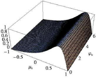
(a) (b)

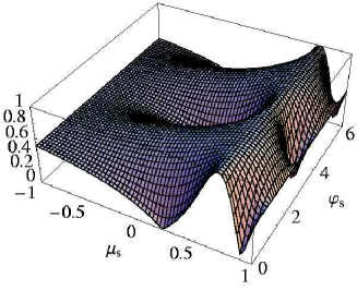
Figure 1: Polarization magnitude of the radiation field produced by Thomson scattering of a beam incident along the $z$-direction on an electron with velocity $0.7c$ also along the $z$-direction, for the following two cases of the polarization state of the incident beam: (a) $Q=U=V=0$, (b) $Q/I=1/2,\;U=V=0$ (where the Stokes parameters are defined in the basis $\bm{\epsilon}_{1}=\bm{x},\,\bm{\epsilon}_{2}=\bm{y}$).

Fig. 1 illustrates the results of using this procedure to compute the polarization magnitude $\Pi(\mu_{s},\varphi_{s})$ of the radiation field produced by Thomson scattering of a polarized beam incident along the $z$-direction (in lab) on a relativistic electron, as a function of the polar angles ($\mu_{s}=\cos\theta_{s},\,\varphi_{s}$) of the scattered photon about the $z$-axis (see Eqn. (195)). The Thomson scattered radiation field in the electron rest frame is derived in the next section. The polarization matrix of the scattered beam in the electron rest frame was computed, as given in Eqn. (191), and then boosted to lab frame, where the polarization magnitude was computed. The polarization magnitude is a scalar and thus changes under the boost due entirely to the aberration of the photon direction.

(a) (b)

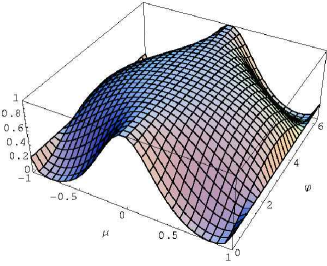
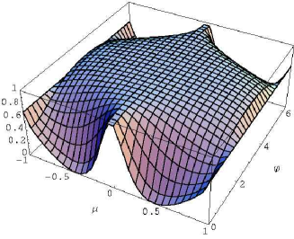
(c) (d)

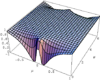
Figure 2: Polarization magnitude of the radiation field produced by Thomson scattering of an unpolarized beam incident along the $z$-direction scattering from an electron moving along the $x$-direction with velocity (a) zero, (b) $0.4c$, (c) $0.9c$, (d) $0.99c$.

V Thomson scattering

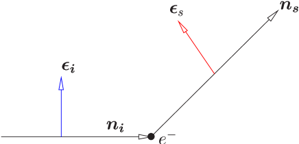
Figure 3: Thomson scattering of a pure incident beam from an electron at rest into a specified final polarization state.

In this section we present a derivation of the equation for the time evolution of the distribution function polarization tensor due to Thomson scattering from a distribution of stationary electrons, starting from the classical results for Thomson scattering, ignoring the effects of electron recoil and induced scattering. Note that throughout this and subsequent sections we work in flat spacetime.

Recall that for a completely linearly polarized beam, $Q^{\mu\nu}\epsilon^{\ast}_{\mu}\epsilon_{\nu}$ is the time-average energy density for electromagnetic radiation of polarization $\epsilon_{\mu}$, where $\epsilon_{\mu}$ is spacelike and normalized, $\vec{\epsilon}^{\ \ast}\cdot\vec{\epsilon}\equiv g^{\mu\nu}\epsilon^{\ast}_{\mu}\epsilon_{\nu}=1$. Consider a completely polarized beam with polarization vector $\vec{\epsilon}_{i}$ and momentum $\vec{p}_{i}$ incident upon an electron at rest (Fig. 3). The polarization matrix of the incident beam is $Q_{i}\vec{\epsilon}_{i}\otimes\vec{\epsilon}_{i}^{\ast}$ where $cQ_{i}$ is the incident flux (we choose units such that $c=1$). Normalization of the polarization vector implies $Q_{i}=Q_{i}^{\mu\nu}\epsilon^{\ast}_{i\,\mu}\epsilon_{i\,\nu}$. In the Thomson limit, in which the electron recoil is negligible, the differential cross section for Thomson scattering of a beam into final momentum $\vec{p}_{s}$ and polarization xs$\vec{\epsilon}_{s}$ is (Jackson, 1998)

$$\frac{d\sigma}{d\Omega_{s}}=\frac{3\sigma_{\rm T}}{8\pi}\left|\vec{\epsilon}^{\ \ast}_{i}\cdot\vec{\epsilon}_{s}\right|^{2}\ .$$ (179)

Thus the power per unit solid angle in the scattered beam is

$${dP_{s}\over d\Omega_{s}}={3\sigma_{\rm T}\over 8\pi}\,Q_{i}\left|\vec{\epsilon}^{\ \ast}_{i}\cdot\vec{\epsilon}_{s}\right|^{2}$$ (180)

where $d\Omega_{s}$ is the element of solid angle associated with the direction of $\vec{p}_{s}$. We may also write $Q_{i}|\vec{\epsilon}^{\ \ast}_{i}\cdot\vec{\epsilon}_{s}|^{2}=Q_{i}^{\mu\nu}\epsilon^{\ast}_{s\,\mu}\epsilon_{s\,\nu}$.

Next consider a gas of electrons all at rest with number density $n_{e}$: we work in the rest frame of the electrons throughout this section. Assuming incoherent scattering, multiplying Eqn. (180) by $n_{e}d\Omega_{s}$ converts scattered power per electron to the rate of change of energy density in final polarization state $\vec{\epsilon}_{s}$:

$${dQ_{s}^{\mu\nu}\over dt}\,\epsilon^{\ast}_{s\,\mu}\epsilon_{s\,\nu}={3\sigma_{\rm T}\over 8\pi}n_{e}Q_{i}^{\mu\nu}\epsilon^{\ast}_{s\,\mu}\epsilon_{s\,\nu}\,d\Omega_{s}\ .$$ (181)

Note that the time derivative $d/dt$ here should actually be interpreted as a total derivative taken along the ray, $d/dt=\partial/\partial t+\bm{n}\cdot\bm{\nabla}$, since eventually the left hand side of the evolution equation will be replaced with the left hand side of Eqn. (205). Using equation (98), and setting $p_{i}=p_{s}$ since we are working in the Thomson limit, we may convert this to the change in the phase space density matrix, giving

$${df_{s}^{\mu\nu}\over dt}\,\epsilon^{\ast}_{s\,\mu}\epsilon_{s\,\nu}d\Omega_{s}={3\sigma_{\rm T}\over 8\pi}n_{e}f_{i}^{\mu\nu}\epsilon^{\ast}_{s\,\mu}\epsilon_{s\,\nu}\,d\Omega_{i}d\Omega_{s}\ .$$ (182)

We would like an equation for the change in $f_{\mu\nu}$ due to scattering, but Eqn. (182) gives the change only for a particular (but arbitrary) polarization of the outgoing wave, $\vec{\epsilon}_{s}$. We cannot remove the polarization factors and conclude $df_{s}^{\mu\nu}\propto f_{i}^{\mu\nu}$ because the polarization of the incoming wave does not lie in the same plane as the polarization of the scattered wave. For a given outgoing momentum $\vec{p}_{s}$, the outgoing polarization is a linear combination of the two basis vectors $\vec{\epsilon}_{1}$ and $\vec{\epsilon}_{2}$ (associated with the photon of momentum $\vec{p}_{s}$) of §III. Thus, $f_{i}^{\mu\nu}\epsilon^{\ast}_{s\,\mu}\epsilon_{s\,\nu}$ projects out of the incoming density matrix $f_{i}^{\mu\nu}$ only those components lying in the $\vec{\epsilon}_{1}$-$\vec{\epsilon}_{2}$ plane. This projection is equivalent to first projecting $f_{i}^{\mu\nu}$ with $\vec{\epsilon}_{1}\otimes\vec{\epsilon}_{1}+\vec{\epsilon}_{2}\otimes\vec{\epsilon}_{2}$. But this is exactly the projection tensor of Eqn. (113), with $\vec{p}=\vec{p}_{s}$ being the outgoing photon momentum and $\vec{v}$ being the electron 4-velocity. Projecting the final polarization vector with $P_{\mu\nu}$ does not change it: $P^{\mu}_{\ \ \alpha}\epsilon_{s\,\mu}=\epsilon_{s\,\alpha}$. It follows that $f_{i}^{\mu\nu}\epsilon^{\ast}_{s\,\mu}\epsilon_{s\,\nu}=f_{i}^{\alpha\beta}P^{\mu}_{\ \ \alpha}P^{\nu}_{\ \ \beta}\epsilon^{\ast}_{s\,\mu}\epsilon_{s\,\nu}$. Now it is safe to remove the outgoing polarization vectors from Eqn. (182).

We conclude that, for any initial and final polarizations,

$${df_{s}^{\mu\nu}(\vec{p}_{s},\vec{v}_{e})\over dt}={3\sigma_{\rm T}\over 8\pi}n_{e}\,P^{\mu}_{\ \ \alpha}(\vec{p}_{s},\vec{v}_{e}\,)P^{\nu}_{\ \ \beta}(\vec{p}_{s},\vec{v}_{e}\,)\,\int d\Omega_{i}\,f_{i}^{\alpha\beta}(\vec{p}_{i},\vec{v}_{e})\ .$$ (183)

Eqn. (183) is the key result for Thomson scattering in the polarization tensor formalism. It gives the photon scattering rate per unit volume for given momenta and polarizations.

If this argument seems a little dry, we note that the appearance of these projection tensor follows straightforwardly from elementary classical electrodynamics. Consider scattering of a quasi-monochromatic beam with central frequency $\omega$ incident in direction $\bm{n}^{(i)}$ by a single electron at rest. Let the complex amplitude of the (analytic signal of the) incident electric field be $\bm{E}^{(i)}(t)$, with $\bm{E}^{(i)}\cdot\bm{n}^{(i)}=0$. The incident wavevector is $\bm{k}=\omega\bm{n}^{(i)}/c$. The complex dipole moment of the radiating electron induced by the incoming wave is $\bm{p}=(e^{2}/m\omega^{2})\bm{E}^{(i)}$. The analytic signal of the electric field of the dipole radiation in the far field produced by the oscillating electron (the scattered field) at position $\bm{x}^{\prime}=x^{\prime}\bm{n}_{s}$ is, using the formula for electric dipole radiation (Jackson, 1998),

$$\bm{E}_{s} = \frac{\mu_{0}}{4\pi}\frac{e^{i\omega x^{\prime}/c}e^{i\omega t}}{x^{\prime}}\omega^{2}\left[\bm{p}-(\bm{n}_{s}\cdot\bm{p})\bm{n}_{s}\right]\ .$$ (184)

The matrix $Q_{ij}$ matrix of the scattered beam is thus given by

$$x^{\prime 2}d\Omega^{\prime}\;Q_{ij}(\bm{n}_{s}) = x^{\prime 2}d\Omega^{\prime}\;\langle E_{r,i}E_{r,j}^{*}\rangle$$ (185)

$$= \frac{3}{4\pi}\sigma_{T}d\Omega^{\prime}\;\left[\bm{P}(\bm{n_{s}})\langle\bm{Q}(\bm{n}^{(i)})\rangle\bm{P}(\bm{n_{s}})\right]_{ij}\ ,$$

where $\sigma_{T}=(e^{2}/mc^{2})^{2}/12\pi\epsilon_{0}^{2}$ is the Thomson cross section (in SI units), and we have defined

$$\left[\bm{Q}(\bm{n}^{(i)})\right]_{ij} = \langle E_{i}^{(i)}(t)E_{j}^{(i)}(t)\rangle$$

$$\left[\bm{P}(\bm{n}_{s})\right]_{ij} = \delta_{ij}-[\bm{n}_{s}]_{i}[\bm{n}_{s}]_{j}\ .$$ (186)

The matrix $\bm{P}(\bm{n}_{s})$ is the projection tensor we saw before, which can be thought of as selecting the components of the incoming field which are transverse to the wavevector of the scattered field. The extension to a arbitrary “polychromatic” incident beam with frequencies not restricted to a small waveband follows provided the electric field components in seperate wavebands are completely uncorrelated.

If the integration time is sufficiently short that we can ignore multiple scatterings, we may replace $n_{e}\sigma_{\rm T}\,dt$ in Eqn. (183) with the optical depth to Thomson scattering, $\tau$. Then we have

$$f_{s}^{\mu\nu}(\vec{p}_{s},\vec{v}_{e})={3\tau\over 8\pi}\,P^{\mu}_{\ \ \alpha}(\vec{p}_{s},\vec{v}_{e}\,)P^{\nu}_{\ \ \beta}(\vec{p}_{s},\vec{v}_{e}\,)\,\int d\Omega_{i}\,f_{i}^{\alpha\beta}(\vec{p}_{i},\vec{v}_{e})\ .$$ (187)

It follows that scattering of a photon with a given incident momentum $\vec{p}_{i}$ leads to a scattered beam with normalized polarization tensor

$$\phi_{s}^{\mu\nu}(\vec{p}_{s},\vec{v}_{e})=\frac{P^{\mu}_{\ \ \alpha}(\vec{p}_{s},\vec{v}_{e}\,)P^{\nu}_{\ \ \beta}(\vec{p}_{s},\vec{v}_{e}\,)\,\phi_{i}^{\alpha\beta}(\vec{p}_{i},\vec{v}_{e})}{P_{\gamma\delta}(\vec{p}_{s},\vec{v}_{e}\,)\phi_{i}^{\gamma\delta}(\vec{p}_{i},\vec{v}_{e})}\ .$$ (188)

Taking the trace of the scattering rate Eqn. (183) yields the evolution equation for the scalar distribution functions $f_{i}(\vec{p}_{i})=g_{\alpha\beta}f_{i}^{\alpha\beta}(\vec{p}_{i})$, $f_{s}(\vec{p}_{i})=g_{\alpha\beta}f_{s}^{\alpha\beta}(\vec{p}_{s})$, which may be written in the following form (by definition of the differential scattering cross section):

$$\frac{d}{dt}(f_{s}\,d^{3}x\,d^{3}p_{s})=(n_{e}\,d^{3}x)\,\frac{d\sigma}{d\Omega_{s}}\,d\Omega_{s}\,(f_{i}\,d^{3}p_{i})\ ,$$ (189)

which yields the differential scattering cross section in the rest frame (and the Thomson limit):

$$\frac{d\sigma}{d\Omega_{s}}=\frac{3\sigma_{\rm T}}{8\pi}\;P_{\alpha\beta}(\vec{p}_{s},\vec{v}_{e})\phi_{i}^{\alpha\beta}(\vec{p}_{i},\vec{v}_{e})\ .$$ (190)

In rest frame coordinates, we may deal with $3\times 3$ matrices rather than tensors. Then we may write the normalized polarization matrix of the scattered beam in terms of that of the incident beam as:

$$\bm{\phi}_{s}(\bm{n}_{s})=\frac{\bm{P}(\bm{n}_{s})\bm{\phi}_{i}(\bm{n}_{i})\bm{P}(\bm{n}_{s})}{\mbox{Tr}[\bm{P}(\bm{n}_{s})\bm{\phi}_{i}(\bm{n}_{i})]}\ .$$ (191)

The polarization magnitude of the beam reduces to a familiar form in the case of an unpolarized incident beam. For example, consider the case of an unpolarized beam incident in the $z$-direction in the rest frame, and let the rest frame direction vector of the scattered beam have components

$$\bm{n}_{s}=(\cos\varphi_{s}\sqrt{1-\mu_{s}^{2}},\sin\varphi_{s}\sqrt{1-\mu_{s}^{2}},\mu_{s})\ .$$ (192)

The incident normalized polarization matrix is $\bm{\phi}(\bm{n}_{i})=\bm{P}(\bm{n}_{i})/2$.

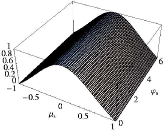
(a) (b)

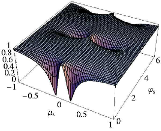
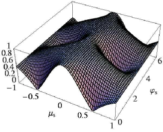
(c) (d)

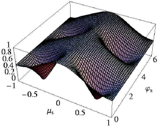
Figure 4: Polarization magnitude versus rest frame scattering angles (in polar coordinates). The plots for incident beams with Stokes parameters: (a) $Q=U=V=0$, (b) $Q/I=0.9,\;U=V=0$, (c) $Q/I=0.5,\;U=V=0$, (d) $U/I=0.5,\;Q=V=0$ .

The polarization magnitude of the scattered beam is given by

$$\Pi^{2}(\mu_{s},\varphi_{s})=2\mbox{Tr}[\bm{\phi}_{s}^{2}]/\mbox{Tr}[\bm{\phi}_{s}]^{2}-1=\left(\frac{1-\mu_{s}^{2}}{1+\mu_{s}^{2}}\right)^{2}\ ,$$ (193)

which is independent of $\varphi_{s}$ since the incident unpolarized beam picks out no preferred azimuth. In the case of an incident beam with a general polarization state, we may choose polarization basis 3-vectors for the incident beam $\bm{\epsilon}_{1}=\bm{e}_{x},\,\bm{\epsilon}_{2}=\bm{e}_{y}$ and write, in the $2\times 2$ polarization subspace,

$$\bm{\phi}_{i}=\frac{1}{2I}\left(\begin{array}[]{cc}I+Q&U+iV\\ U-iV&I-Q\end{array}\right)\ .$$ (194)

Then we find the scattered polarization magnitude

$$\Pi^{2}(\mu_{s},\varphi_{s})=1+\frac{4\,\left(-I^{2}+Q^{2}+U^{2}+V^{2}\right)\,{\mu_{s}}^{2}}{I^{2}{\left[1+{\mu_{s}}^{2}+\left(-1+{\mu_{s}}^{2}\right)\left(Q\,\cos(2\,\varphi_{s})+U\,\sin(2\,\varphi_{s})\right)/I\right]}^{2}}\ .$$ (195)

This may also be written as

$$\Pi^{2}(\mu_{s},\varphi_{s})=1+\frac{\left(-I^{2}+Q^{2}+U^{2}+V^{2}\right)\,{\mu_{s}}^{2}}{I^{2}{\left[1-n_{si}n_{sj}\phi_{i}^{ij}\right]}^{2}}\ .$$ (196)

This function is plotted for incident beams with various polarization states in Fig. 4.

From Eqn. (191) we can determine the probability for a photon to Thomson scatter into a particular solid angle element $d\Omega_{s}$, which is conventionally termed the phase function. This is simply proportional to the differential cross section, which in matrix notation is

$$\frac{d\sigma}{d\Omega_{s}}=\frac{3\sigma_{\rm T}}{8\pi}\;\mbox{Tr}[\bm{\phi}_{i}(\bm{n}_{i})\bm{P}(\bm{n}_{s})]\ .$$ (197)

Thus the phase function for Thomson scattering is a function of the scattered direction vector $\bm{n}_{s}$ and the elements of the incident polarization matrix $\bm{\phi}_{i}(\bm{n}_{i})$ (the dependence on $\bm{n}_{i}$ is implicit in $\bm{\phi}_{i}(\bm{n}_{i})$). Denoting the phase function as $\Phi[\bm{n}_{s},\bm{\phi}_{i}(\bm{n}_{i})]$, we use the normalization

$$\int\Phi[\bm{n}_{s},\bm{\phi}_{i}(\bm{n}_{i})]\;\frac{d\Omega_{s}}{4\pi}=1\ .$$ (198)

Since $\int P_{ij}(\bm{n}_{s})\;d\Omega_{s}/4\pi=2\delta_{ij}/3$, we have

$$\Phi[\bm{n}_{s},\bm{\phi}_{i}(\bm{n}_{i})]=\frac{3}{2}\;\mbox{Tr}[\bm{\phi}(\bm{n}_{i})\bm{P}(\bm{n}_{s})]\ .$$ (199)

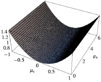
(a) (b)

Figure 5: Phase function $\Phi$ versus rest frame scattering angles (in polar coordinates, for a beam incident along the $z$-axis with Stokes parameters: (a) $Q=U=V=0$, (b) $Q/I=1,\;U=V=0$.

For example, consider the case of an incident beam with $\bm{n}_{i}=(0,0,1)$, and intensity polarization matrix with Stokes parameters defined with respect to polarization basis vectors (associated with the incident beam) $\bm{\epsilon}_{1}=\bm{e}_{x},\,\bm{\epsilon}_{2}=\bm{e}_{y}$:

$$\bm{I}(\bm{n})=\frac{1}{2}\left(\begin{array}[]{ccc}I+Q&U&0\\ U&I-Q&0\\ 0&0&0\end{array}\right)\ .$$ (203)

and let the scattered direction have the components (192). Then we obtain the phase function (Code & Whitney, 1995):

$$\Phi[\bm{n}_{s},\bm{\phi}_{i}(\bm{n}_{i})] = \frac{3}{4}\left[1+\mu_{s}^{2}-\;(1-\mu_{s}^{2})\;\left(Q\cos 2\phi_{s}+U\sin 2\phi_{s}\right)/I\right]\ .$$ (204)

In Fig. 5 this function is compared for unpolarized and completely polarized incident beams. The polarization of the incident beam destroys the azimuthal symmetry of the differential cross section and phase function.

This completes our discussion of the generation of polarization by classical Thomson scattering in the electron rest frame. In the next section we use these results to construct the photon Boltzmann equation for Thomson scattering.

VI Kinetic equation in the Thomson limit

The evolution of the polarization matrix of the radiation field due to Compton scattering is determined by the Boltzmann (or kinetic) equation

$$p^{\alpha}\partial_{\alpha}f_{\mu\nu}=C_{\mu\nu}\ ,$$ (205)

where $C_{\mu\nu}$ is the Compton scattering term. In this section we derive this scattering term for arbitrarily relativistic electrons and polarized photons. In fact, since the CMB photons have negligible momentum in comparison to the electron rest mass, the SZE can be calculated accurately with a simpler scattering term derived in the Thomson limit, in which the electron recoil is ignored. However, we go through the complete relativistic calculation in any case since there are other applications in which the recoil effect cannot be ignored.

We do however ignore the effect of induced (or stimulated) scattering, which is required for example to obtain the Kompaneets equation often used to derive the thermal SZ distortion. But the terms due to induced scattering in the Kompaneets equation are negligible in the case of cluster SZE, and in general in the unpolarized case it is known that induced scattering is a negligible effect unless electron energies are comparable to the electron rest mass. In any case a rigorous derivation of the induced effects require a quantum treatment (Nagirner & Poutanen, 2001), which we have not developed here. We also neglect electron polarization, assuming that frequent Coulomb collisions destroy any spin alignments, and Pauli blocking (which is irrelevant in the regimes of interest).

We now use the preceding results to derive the Boltzmann collision term in the electron rest frame. This is derived by the following heuristic line of reasoning. If we ignore polarization and assign a scalar distribution function $f(\bm{p})$ to each photon, the scattering rate is given by Eqn. (189) with the cross-section for the transition from $\bm{p}_{i}$ to $\bm{p}_{s}$ replaced by its unpolarized form, which in the Thomson limit is

$$\frac{d\sigma}{d\Omega_{s}}=\frac{3\sigma_{\rm T}}{16\pi}\left[1+(\bm{n}_{i}\cdot\bm{n}_{s})^{2}\right]\ .$$ (206)

We could then write the rate of change of phase space density by subtracting from Eqn. (189) the rate of scattering out of $\bm{p}_{s}$. That result is known as the master equation or Boltzmann equation for $f$ (Binney & Tremaine, 1987; Groot et al., 1980):

$$\frac{d}{dt}f(\bm{p})=n_{e}\int d\Omega_{s}\int d^{3}p_{i}\,\frac{d\sigma}{d\Omega_{s}}(\bm{p}_{s};\bm{p}_{i})\,f(\bm{p}_{i})\left[\delta^{3}(\bm{p}_{s}-\bm{p})-\delta^{3}(\bm{p}_{i}-\bm{p})\right]\ .\quad$$ (207)

The meaning of the master equation is that the rate of change of the photon number in a given phase space element is given by summing over all scatterings into and out of this element. In this expression, $\bm{p}_{s}$ is not a free variable, it is a function of the incident photon momentum and scattering angles, $\bm{p}_{s}=\bm{p}_{s}(\bm{p}_{i},\bm{n}_{s})$, determined by the scattering kinematics. In the Thomson limit, $|\bm{p}_{s}|=|\bm{p}_{i}|$, so the scattered photon momentum is simply given by $\bm{p}_{s}(\bm{p}_{i},\bm{n}_{s})=|\bm{p}_{i}|\bm{n}_{s}$. This allows completion of the integral over the first delta function.

The first and second terms inside the square brackets correspond to scatterings into and out of the beam (with momentum $\bm{p}$) respectively, and are termed the gain and loss terms.

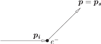
(a) Gain

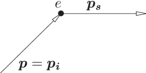
(b) Loss

Figure 6: Gain and loss processes in kinetic/master equation for Thomson scattering.

The delta functions select the appropriate states, as indicated in Fig. 6. Eqn. (207) is simply a statement of photon number conservation combined with the rate of scattering into the final momentum state (189).

Now we wish to generalize this to the polarized case. The polarization tensor allows us to extend equation (207) to a general polarization state. and write down the kinetic equation for polarization corresponding to Eqn. (183). Because the transition rate is linear in $\bm{f}_{i}$ and $\bm{f}_{s}$ it is possible to write the scattering rate for a linear superposition of initial states to a linear superposition of final states. Assuming linear superposition for incoherent light, we can write the most general incident state as $f^{\alpha\beta}(\vec{p}_{i},\vec{v}_{e})$ and ask for the transition rate of each element of this matrix. The transition rate is a linear transformation from $f^{\alpha\beta}(\vec{p}_{i},\vec{v}_{e})$ to $f^{\mu\nu}(\vec{p}_{s},\vec{v}_{e})$ and must therefore take the following form,

$$\frac{d}{dt}[f^{\mu\nu}(\vec{p}_{s},\vec{v}_{e})\,d^{3}p_{s}]=n_{e}\,\Phi^{\mu\nu}_{\alpha\beta}(\vec{p}_{s},\vec{v}_{e};\vec{p}_{i},\vec{v}_{e})\,f^{\alpha\beta}(\vec{p}_{i},\vec{v}_{e})\,d^{3}p_{i}\,d\Omega_{s}\ ,$$ (208)

with some matrix $\Phi^{\mu\nu}_{\alpha\beta}$ that we call the polarization scattering tensor. It is convenient to write this as $\Phi^{\mu\nu}_{\alpha\beta}(s;i)$, where the arguments $(i)$ and $(s)$ are abbreviations for the pairs of 4-vectors $(\vec{p}_{i},\vec{v}_{e})$ and $(\vec{p}_{s},\vec{v}_{e})$,

The polarization scattering tensor is effectively a $4\times 4$ matrix giving the transition rate between all possible initial and final polarization states. It follows from Eqn. (183) that in the Thomson limit the polarization scattering tensor is given by

$$\Phi^{\mu\nu}_{\alpha\beta}(s;i)=\frac{3\sigma_{\rm T}}{8\pi}P^{\mu}_{\ \ \alpha}(\vec{p}_{s},\vec{v}_{e})P^{\nu}_{\ \ \beta}(\vec{p}_{s},\vec{v}_{e})\ .$$ (209)

Now we make the following ansatz for polarized analogue of the master equation corresponding to Eqn. (207):

$$\frac{d}{dt}f^{\mu\nu}(\vec{p},\vec{v}_{e})=n_{e}\int\!d\Omega_{s}\int\!d^{3}p_{i}\,\Phi^{\alpha\beta}_{\gamma\delta}(\vec{p}_{s},\vec{v}_{e};\vec{p}_{i},\vec{v}_{e})\,f^{\gamma\delta}(\vec{p}_{i},\vec{v}_{e})\quad\quad$$

$$\quad\quad\quad\quad\times\left[\delta^{\mu}_{\ \,\alpha}\delta^{\nu}_{\ \,\beta}\,\delta^{3}(\bm{p}_{s}-\bm{p})-g_{\alpha\beta}\,\phi^{\mu\nu}(\vec{p},\vec{v}_{e})\,\delta^{3}(\bm{p}_{i}-\bm{p})\right]\ .$$ (210)

This is the rest frame form of the scattering term $C^{\mu\nu}$ in Eqn. (205). With this ansatz for the master equation, it may be checked that for any two initial and scattered pure states $f^{\alpha\beta}(\vec{p}_{i},\vec{v}_{e})=f_{i}\epsilon_{i}^{\alpha}(\epsilon_{i}^{\beta})^{\ast}$ and $f^{\mu\nu}(\vec{p}_{s},\vec{v}_{e})=f_{s}\epsilon_{s}^{\mu}(\epsilon_{s}^{\nu})^{\ast}$, Eqn. (VI) reduces to Eqn. (207) with the Thomson cross section Eqn. (190). Then since any polarized beam can be written as some superposition of pure states, it follows that Eqn. (VI) is true for all polarization states. This verifies that the ansatz (VI) is correct in the Thomson limit.

The first term in the square brackets is exactly the gain term of Eqn. (183). The second term represents losses to any final polarization state; the sum over polarizations is given by $g_{\alpha\beta}$. Each incident photon beam with polarization tensor $\phi^{\mu\nu}(\vec{p},\vec{v}_{e})$ is lost by scattering implying that the loss term must be proportional to $\phi^{\mu\nu}(\vec{p},\vec{v}_{e})$. Just as the loss term in Eqn. (207) is proportional to the same quantity occurring on the left-hand side of the equation, the same is true here. In fact this loss term is simply the phase function multiplied by the incident beam, and is thus proportional to the probability of a photon scattering from momentum $\vec{p}_{i}$ to $\vec{p}_{s}$. To see this, note that the loss term contains the scalar obtained by contracting the projection tensors which are orthogonal to the incident and scattered photons:

$$P^{\alpha\beta}(\vec{p}_{i},\vec{v}_{e})P_{\alpha\beta}(\vec{p}_{s},\vec{v}_{e})=2+\frac{2}{p_{i}p_{s}}\;\vec{p}_{i}\cdot\vec{p}_{s}+\frac{(\vec{p}_{i}\cdot\vec{p}_{s})^{2}}{(p_{i}p_{s})^{2}}\ .$$ (211)

where $p_{i}\equiv-\vec{p}_{i}\cdot\vec{v}_{e}$, $p_{s}\equiv-\vec{p}_{s}\cdot\vec{v}_{e}$. In the rest frame of $\vec{v}_{e}$, $p_{i}^{\mu}=p_{i}(1,\mbox{\boldmath$n$}_{i})$, $p_{s}^{\mu}=p_{s}(1,\mbox{\boldmath$n$}_{s})$, giving $\vec{p}_{i}\cdot\vec{p}_{s}=-p_{i}p_{s}(1-\mbox{\boldmath$n$}_{i}\cdot\mbox{\boldmath$n$}_{s})$, and the loss term scalar has the form

$$P^{\alpha\beta}(\vec{p}_{i},\vec{v}_{e})P_{\alpha\beta}(\vec{p}_{s},\vec{v}_{e})=1+(\mbox{\boldmath$n$}_{i}\cdot\mbox{\boldmath$n$}_{s})^{2}\ ,$$ (212)

which is the familiar angular dependence of the differential cross section for Thomson scattering of unpolarized radiation. The total loss term is thus simply proportional to the incident beam multiplied by the total cross section (in this case, since we have restricted to the Thomson limit, the Thomson cross section).

Note that the form of Eqn. (VI) guarantees photon number conservation (Compton scattering cannot change the overall photon number):

$$\int d^{3}p\;g_{\mu\nu}\frac{df^{\mu\nu}(\vec{p},\vec{v}_{e})}{dt}=0\ .$$ (213)

Integration over the delta functions yields the much simplified form of the rest frame kinetic equation :

$$\frac{d}{dt}f^{\mu\nu}(\vec{p},\vec{v}_{e})=n_{e}\sigma_{\rm T}\Biggl{[}\frac{3}{2}\int\!\frac{d\Omega_{i}}{4\pi}\,P^{\mu}_{\ \ \alpha}(\vec{p},\vec{v}_{e})P^{\nu}_{\ \ \beta}(\vec{p},\vec{v}_{e})f^{\alpha\beta}(\vec{p}_{i},\vec{v}_{e})\Biggr{.}-f^{\mu\nu}(\vec{p},\vec{v}_{e})\Biggr{]}\ .$$ (214)

This equation, in conjunction with the transformation to lab frame and integration over electron velocities, discussed in the next sections, is sufficient to compute all the Sunyaev-Zeldovich effects.

At this point we consider the form of Eqn. (214) in the case where the polarization tensors on the right hand side are taken to be unpolarized. This will be used in Paper II in the computation of the polarization generated by a single scattering of an unpolarized radiation field. In this case the integrand of the gain term in Eqn. (214) is proportional to the following combination of projection tensors:

$$G^{\mu\nu}(\vec{p}_{i},\vec{p}_{s},\vec{v}_{e})\equiv P^{\mu}_{\ \ \alpha}(\vec{p}_{s},\vec{v}_{e})P^{\nu}_{\ \ \beta}(\vec{p}_{s},\vec{v}_{e})P^{\alpha\beta}(\vec{p}_{i},\vec{v}_{e})\ .$$ (215)

In the electron rest frame, the spatial components of the integrand of the gain term are given by

$$G^{ij}(\vec{p}_{i},\vec{p}_{s},\vec{v}_{e}) = \left(\delta^{i}_{k}-n^{i}_{s}n_{s,k}\right)\left(\delta^{j}_{l}-n^{j}_{s}n_{s,l}\right)\left(\delta^{kl}-n^{k}_{i}n^{l}_{i}\right)$$ (216)

$$= (\delta^{ij}-n^{i}_{i}n^{j}_{i})-n^{i}_{s}n_{s}^{j}[1+(\bm{n}_{s}\cdot\bm{n}_{i})^{2}]+(n^{i}_{s}n^{j}_{s}+n^{j}_{s}n^{i}_{s})(\bm{n}_{s}\cdot\bm{n}_{i})\ .\quad\quad\quad$$

This form is convenient for the calculation of the polarization generated by scattering of the CMB quadrupole, in the companion paper (and, for example, in (Portsmouth, 2004)).

We close this section with a demonstration that the rest frame form of the kinetic equation, Eqn. (214), yields the well known results of Chandrasekhar (1960) for the polarized radiative transfer equations in the case of Thomson scattering from cold (i.e. stationary) electrons in a slab geometry. Since Chandrasekhar used a different formalism based on transformations of the Stokes parameters to derive his expressions, this is an important check of the formalism we have developed. These equations also yield the form of the scattering term for the polarization in the primary CMB calculation.

Consider a plane parallel atmosphere of cold electrons with uniform density filling the half-space $z<0$, illuminated by an unpolarized beam of monochromatic radiation incident along the normal to the plane (we do not specify the boundary conditions here, since we are only interested in deriving the form of the transfer equations and not their solution). By symmetry the radiation field in this case is clearly axisymmetric. We work entirely in the electron rest frame, where $I^{00}=I^{0i}=0$, and following Chandrasekhar (1960) define $\tau$ to be the optical depth from the surface $z=0$ along the downward normal. The Cartesian coordinates in the plane are $x$ and $y$, and The polar and azimuthal angles about the $z$-axis are denoted $\theta$ and $\varphi$ (and $\mu=\cos\theta$).

Then the kinetic equation for the lab frame intensity polarization matrix $\bm{I}(\mu,\varphi,\tau)$ is given by Eqn. (214) (replacing distribution function tensors by intensity tensors, which is trivially allowed here since the beam is monochromatic):

$$\mu\;\partial_{\tau}\bm{I}(\mu,\varphi,\tau) = -\frac{3}{2}\bm{P}(\bm{n})\int_{-1}^{1}d\mu_{s}\;\int_{0}^{2\pi}\frac{d\varphi_{s}}{4\pi}\bm{I}(\mu_{s},\varphi_{s},\tau)\bm{P^{T}}(\bm{n})+\;\bm{I}(\mu,\varphi,\tau)\ .$$

where $\bm{n}(\theta,\varphi)=(\cos\varphi\sin\theta,\sin\varphi\sin\theta,\cos\theta)$ is the direction 3-vector of the beam. Note that in this expression, following Chandrasekhar (1960), the gain and loss terms have picked up a minus sign since the direction of increasing optical depth (along the normal to the boundary $z=0$ directed into the half-space $z<0$) is defined to be opposite to the polar axis.

In contrast to the Stokes vector approach of Chandrasekhar (1960), the polarization matrix even in this azimuthally symmetric problem has azimuthal dependence. But we are free to exploit the azimuthal symmetry here by choosing a convenient azimuth to evaluate the projection factors, and then the result obtained for this azimuth may be transformed into the other directions trivially. Choosing $\varphi=0$, we have $(n^{x},n^{y},n^{z})=(\sqrt{1-\mu^{2}},0,\mu)$. In the $\varphi=0$ direction, $I^{ij}$ has the form (since the $yx$ and $yz$ cross-terms must vanish in order that the place of polarization is parallel or perpendicular to the $y-z$ plane as required by axisymmetry).

$$\bm{I}(\mu,0,\tau)=\left(\begin{array}[]{ccc}I_{l}\mu^{2}&0&I_{l}\mu\sqrt{1-\mu^{2}}\\ 0&I_{r}&0\\ I_{l}\mu\sqrt{1-\mu^{2}}&0&I_{l}(1-\mu^{2})\end{array}\right)\ .$$ (218)

Here $I_{l}(\mu,\tau)$ and $I_{r}(\mu,\tau)$ are the azimuth independent Stokes parameters, parallel and perpendicular respectively to the meridian plane, as defined in Chandrasekhar (1960). The matrices inside the $d\varphi_{s}$ integrals range over all values of $\varphi_{s}$ though, so an expression for $I^{kl}(\mu_{s},\varphi_{s},\tau)$ is required. By azimuthal symmetry, this is simply given by rotating $I^{kl}(\mu_{s},0,\tau)$ through an angle $\varphi_{s}$ about the $\hat{z}$ axis (since under rotation polarization matrices transform according to the vector rotation of the electric field strength vectors):

$$\bm{I}(\mu_{s},\varphi_{s},\tau)=\bm{R}(-\varphi_{s}\hat{z})\bm{I}(\mu_{s},0,\tau)\bm{R^{T}}(\varphi_{s}\hat{z})\ .$$ (219)

where $\bm{R}(\varphi_{s}\hat{z})$ is the matrix which rotates through angle $\varphi_{s}$ about the $z$-axis.

$$\bm{I}(\mu_{s},\varphi_{s},\tau) =\left[\begin{array}[]{ccc}I_{l}\mu_{s}^{2}\cos^{2}\varphi_{s}+I_{r}\sin^{2}\varphi_{s}&-I_{l}\mu_{s}^{2}\sin\varphi_{s}\cos\varphi_{s}+I_{r}\cos\varphi_{s}\sin\varphi_{s}&I_{l}\mu_{s}\sqrt{1-\mu_{s}^{2}}\cos\varphi_{s}\\ -I_{l}\mu_{s}^{2}\cos\varphi_{s}\sin\varphi_{s}+I_{r}\cos\varphi_{s}\sin\varphi_{s}&I_{l}\mu_{s}^{2}\sin^{2}\varphi_{s}+I_{r}\cos^{2}\varphi_{s}&-I_{l}\mu_{s}\sqrt{1-\mu_{s}^{2}}\sin\varphi_{s}\\ I_{l}\mu_{s}\sqrt{1-\mu_{s}^{2}}\cos\varphi_{s}&-I_{l}\mu_{s}\sqrt{1-\mu_{s}^{2}}\sin\varphi_{s}&I_{l}(1-\mu_{s}^{2})\end{array}\right]$$ (223)

Evaluating the $I^{xx}$ component first, we obtain

$$\mu\;\partial_{\tau}I^{xx}(\mu,0,\tau) = -\frac{3}{2}\int_{-1}^{1}d\mu_{s}\;\int_{0}^{2\pi}\frac{d\varphi_{s}}{4\pi}S^{xx}(\mu,\mu_{s},\varphi_{s},\tau)+\;I^{xx}(\mu,0,\tau)\ ,$$ (225)

where

$$S^{xx}(\mu,\mu_{s},\varphi_{s},\tau) = (\delta^{x}_{\;\;\;k}-n^{x}n_{k})(\delta^{x}_{\;\;\;l}-n^{x}n_{l})\;\;I^{kl}(\mu_{s},\varphi_{s},\tau)$$

$$= \mu^{4}I^{xx}(\mu_{s},\varphi_{s},\tau)+\mu^{2}(1-\mu^{2})I^{zz}(\mu_{s},\varphi_{s},\tau)-2\mu(1-\mu^{2})^{3/2}I^{xz}(\mu_{s},\varphi_{s},\tau)\ .$$

Breaking this into three terms for clarity

$$\mu\;\partial_{\tau}I^{xx}(\mu,0,\tau) = \mu^{3}\;\partial_{\tau}I_{l}(\mu,\tau)$$ (227)

$$= -\frac{3}{2}\int_{-1}^{1}d\mu_{s}\;\int_{0}^{2\pi}\frac{d\varphi_{s}}{4\pi}\;\;S^{xx}(\mu,\mu_{s},\varphi_{s},\tau)+\;I^{xx}(\mu,0,\tau)$$

$$= I_{1}(\mu,\tau)+I_{2}(\mu,\tau)+I_{3}(\mu,\tau)+\mu^{2}\;I_{l}(\mu,\tau)\ ,$$

where

$$I_{1}(\mu,\tau) = -\frac{3}{2}\mu^{4}\int_{-1}^{1}d\mu_{s}\;\int_{0}^{2\pi}\frac{d\varphi_{s}}{4\pi}\;\;\left(I_{l}(\mu_{s},\tau)\mu_{s}^{2}\cos^{2}\varphi_{s}+I_{r}(\mu_{s},\tau)\sin^{2}\varphi_{s}\right)$$

$$= -\frac{3}{8}\mu^{4}\int_{-1}^{1}d\mu_{s}\;\;\left(I_{l}(\mu_{s},\tau)\mu_{s}^{2}+I_{r}(\mu_{s},\tau)\right)\ ,$$

$$I_{2}(\mu,\tau) = -\frac{3}{2}\mu^{2}(1-\mu^{2})\int_{-1}^{1}d\mu_{s}\;\int_{0}^{2\pi}\frac{d\varphi_{s}}{4\pi}\;\;I_{l}(\mu_{s},\tau)(1-\mu_{s}^{2})$$

$$= -\frac{3}{4}\mu^{2}(1-\mu^{2})\int_{-1}^{1}d\mu_{s}\;I_{l}(\mu_{s},\tau)(1-\mu_{s}^{2})\ ,$$

$$I_{3}(\mu,\tau) = 3\mu(1-\mu^{2})^{3/2}\int_{-1}^{1}d\mu_{s}\;\int_{0}^{2\pi}\frac{d\varphi_{s}}{4\pi}\;\;\;I_{l}(\mu_{s},\tau)\mu_{s}\sqrt{1-\mu_{s}^{2}}\cos\varphi_{s}$$ (228)

$$= 0\ .$$

Adding the three terms above and dividing by $\mu^{2}$ gives

$$\!\!\!\!\!\!\!\!\!\!\!\!\!\!\!\!\!\mu\;\partial_{\tau}I_{l}(\mu,\tau) = I_{l}(\mu,\tau)-\frac{3}{8}\int_{-1}^{1}d\mu_{s}\;\;\biggl{\{}I_{l}(\mu_{s},\tau)\left[2(1-\mu_{s}^{2})(1-\mu^{2})+\mu^{2}\mu_{s}^{2}\right]+I_{r}(\mu_{s},\tau)\mu^{2}\biggr{\}}\ .$$ (229)

The equation for $I_{r}$ is obtained similarly from the evolution of the $I^{yy}$ component,

$$\mu\;\partial_{\tau}I^{yy}(\mu,0,\tau) = -\frac{3}{2}\int_{-1}^{1}d\mu_{s}\;\int_{0}^{2\pi}\frac{d\varphi_{s}}{4\pi}S^{yy}(\mu,\mu_{s},\varphi_{s},\tau)+\;I^{yy}(\mu,0,\tau)\ ,$$ (230)

where

$$S^{yy}(\mu,\mu_{s},\varphi_{s},\tau) = (\delta^{y}_{\;\;\;k}-n^{y}n_{k})(\delta^{y}_{\;\;\;l}-n^{y}n_{l})\;\;I^{kl}(\mu_{s},\varphi_{s},\tau)$$ (231)

$$= I^{yy}(\mu_{s},\varphi_{s},\tau)\ .$$

Therefore

$$\mu\;\partial_{\tau}I^{yy}(\mu,0,\tau) = \mu\;\partial_{\tau}I_{r}(\mu,\tau)$$ (232)

$$= I_{r}(\mu,0,\tau)-\frac{3}{2}\int_{-1}^{1}d\mu_{s}\;\int_{0}^{2\pi}\frac{d\varphi_{s}}{4\pi}\;\;\left(I_{l}(\mu_{s},\tau)\mu_{s}^{2}\sin^{2}\varphi_{s}+I_{r}(\mu_{s},\tau)\cos^{2}\varphi_{s}\right)$$

$$= I_{r}(\mu,0,\tau)-\frac{3}{8}\int_{-1}^{1}d\mu_{s}\;\biggl{\{}I_{l}(\mu_{s},\tau)\mu_{s}^{2}+I_{r}(\mu_{s},\tau)\biggr{\}}\ .$$

Eqns. (229) and (232) are the coupled radiative transfer equations for the Stokes parameters for Thomson scattering in slab geometry, first obtained by Chandrasekhar Chandrasekhar (1960).

These equations also yield straightforwardly the form of the polarization scattering term in the Boltzmann equation for the evolution of the primary CMB anisotropies, in the form given (but not derived) in (Dodelson, 2003), as follows. In a frame in which the $\bm{k}$-mode considered is aligned with the local $\bm{z}$-axis, and the observation direction is $\bm{n}=(\sqrt{1-\mu^{2}},0,\mu)$, the form of the polarization matrix of the CMB is:

$$\bm{I}(\mu)=\frac{1}{2}\left(\begin{array}[]{ccc}(I-\Pi)\mu^{2}&0&(I-\Pi)\mu\sqrt{1-\mu^{2}}\\ 0&I+\Pi&0\\ (I-\Pi)\mu\sqrt{1-\mu^{2}}&0&(I-\Pi)(1-\mu^{2})\end{array}\right)\ ,$$ (233)

where we have defined the total intensity $I=I_{l}+I_{r}$ and total polarization intensity $\Pi=I_{l}-I_{r}$. The polarization magnitude $\Pi$ is obvously independent of $\varphi$ in this azimuthally symmetrical situation. Using the previous equations for $I_{l}$ and $I_{r}$, we find

$$\dot{\Pi} = \Pi-\frac{3}{8}(1-\mu^{2})\int_{-1}^{1}d\mu^{\prime}\left[I_{l}(3\mu^{\prime 2}-1)-I_{l}+I_{r}\right]$$ (234)

$$= \Pi-\frac{1}{2}\left(1-P_{2}(\mu)\right)\int_{-1}^{1}\frac{d\mu^{\prime}}{2}\left[IP_{2}(\mu^{\prime})+\Pi\left(P_{2}(\mu^{\prime})-P_{0}(\mu^{\prime})\right)\right]\ .$$

Following (Dodelson, 2003), we define

$$\Delta_{l}\equiv(-i)^{l}\int_{1}^{-1}\frac{d\mu^{\prime}}{2}IP_{l}(\mu^{\prime})\ ,$$

$$\Delta_{Pl}\equiv(-i)^{l}\int_{1}^{-1}\frac{d\mu^{\prime}}{2}\Pi P_{l}(\mu^{\prime})\ .$$ (235)

With $\Pi=\Delta_{P}$, we obtain the standard form of the CMB polarization scattering term,

$$\frac{D}{D\tau}{\Delta}_{P}=-\dot{\tau_{\rm T}}\left[-\Delta_{P}+\frac{1}{2}\left(1-P_{2}(\mu)\right)\left(\Delta_{2}+\Delta_{P2}+\Delta_{P0}\right)\right]\ .$$ (236)

(Note $\tau$ is now conformal time, $\tau_{\rm T}$ is Thomson optical depth, $D/D\tau=\partial/\partial\tau+ik\mu$. The second term in the total derivative comes from the other terms in the Liouville equation).

VII Klein-Nishina scattering

Up to now we have worked in the Thomson limit. In this section we extend to the general case of Compton scattering with the full Klein-Nishina form of the scattering cross section, and taking into account the electron recoil.

For now we work still in the rest frame of the electron before scattering (the “initial” electron). To derive the polarization tensor kinetic equation our starting point is the Klein-Nishina differential cross-section (Greiner & Reinhardt, 1994), in the initial electron rest frame, for photons with 3-momentum $\bm{p}_{i}$ and polarization $\bm{\epsilon}_{i}$ to scatter into 3-momentum $\bm{p}_{s}$ and polarization $\bm{\epsilon}_{s}$, generalized to allow for arbitrary elliptical polarization (Stedman & Pooke, 1982):

$$\frac{d\sigma}{d\Omega_{s}}=\frac{3\sigma_{\rm T}}{8\pi}\left(\frac{p_{s}}{p_{i}}\right)^{2}\Biggl{[}|\bm{\epsilon}_{i}\cdot\bm{\epsilon}_{s}^{\,\ast}|^{2}+\frac{1}{4}\left(\frac{p_{s}}{p_{i}}+\frac{p_{i}}{p_{s}}-2\right)\left(1+|\bm{\epsilon}_{i}\cdot\bm{\epsilon}_{s}^{\,\ast}|^{2}-|\bm{\epsilon}_{i}\cdot\bm{\epsilon}_{s}|^{2}\right)\Biggr{]}\ .$$ (237)

where $p_{i}\equiv E(\bm{p}_{i})=|\bm{p}_{i}|$ and $p_{s}\equiv E(\bm{p}_{s})=|\bm{p}_{i}|$. We allow the polarization vector to be complex in order to treat elliptical polarization; the polarization vectors are normalized by $\bm{\epsilon}_{i}\cdot\bm{\epsilon}_{i}^{\,\ast}=\bm{\epsilon}_{s}\cdot\bm{\epsilon}_{s}^{\,\ast}=1$. The factor $(1+|\bm{\epsilon}_{i}\cdot\bm{\epsilon}_{s}^{\,\ast}|^{2}-|\bm{\epsilon}_{i}\cdot\bm{\epsilon}_{s}|^{2})$ is usually not given as it reduces to unity for linearly polarized light, but we allow for light of arbitrary polarization. Eqn. (237) assumes the transverse gauge condition $\bm{\epsilon}_{i}\cdot\bm{p}_{i}=\bm{\epsilon}_{s}\cdot\bm{p}_{s}=0$ and that the time component of both polarization 4-vectors vanishes in the initial electron rest frame. The factor $(p_{s}/p_{i})^{2}$ in the cross section is a phase space factor.

Conservation of energy-momentum relates the initial and final momenta and scattering angle:

$$\frac{p_{s}}{p_{i}}=\left[1+\frac{p_{i}}{m_{e}}(1-\bm{n}_{i}\cdot\bm{n}_{s})\right]^{-1}=1-\frac{p_{s}}{m_{e}}(1-\bm{n}_{i}\cdot\bm{n}_{s})\ ,$$ (238)

where $\bm{n}_{i}$ and $\bm{n}_{s}$ are unit three-vectors along the spatial parts of the photon momenta $\bm{p}_{i}=p_{i}\bm{n}_{i}$ and $\bm{p}_{s}=p_{s}\bm{n}_{s}$. Note that for fixed directions, $dp_{s}/dp_{i}=(p_{s}/p_{i})^{2}$.

Equations (237) and (238) both assume that all quantities are given in the rest frame of the incident electron. We note, incidentally, that the Klein-Nishina formula should be symmetric under the interchange of the initial and final states, but the gauge condition which was imposed to derive this form of the cross section required that the incident and scattered photon polarization basis 4-vectors be orthogonal to the incident electron, and it thus appears rather asymmetric. However, it is true that there is nothing special about this choice of gauge. In Appendix A, it is demonstrated that the cross section is manifestly symmetric under interchange of the initial and final states.

The 4-velocity of the incident electron will from now on be denoted $\vec{v}_{i}$, rather than $\vec{v}_{e}$ (since now we have to distinguish between the incident and scattered electron momenta). Now following the procedure in the previous section, we write the transition rate of the scattered polarization matrix $f^{\mu\nu}(\vec{p}_{s},\vec{v}_{i})$ as a linear transformation of the incident matrix $f^{\alpha\beta}(\vec{p}_{i},\vec{v}_{i})$, as in Eqns. (208) and (209), except we pull the phase space factor out for convenience:

$$\frac{d}{dt}[f^{\mu\nu}(\vec{p}_{s},\vec{v}_{i})\,d^{3}p_{s}]=n_{e}\,\Phi^{\mu\nu}_{\alpha\beta}(\vec{p}_{s},\vec{v}_{i};\vec{p}_{i},\vec{v}_{i})\,f^{\alpha\beta}(\vec{p}_{i},\vec{v}_{i})\left(\frac{p_{s}}{p_{i}}\right)^{2}d^{3}p_{i}\,d\Omega_{s}\ ,$$ (239)

The scattering polarization tensor $\Phi^{\mu\nu}_{\alpha\beta}$ for the Klein-Nishina cross-section is then given by the modified form:

$$\Phi^{\mu\nu}_{\alpha\beta}(s;i) = \frac{3\sigma_{\rm T}}{8\pi}\Biggl{\{}P^{\mu\nu}_{\alpha\beta}(s)+\frac{1}{4}\left(\frac{p_{s}}{p_{i}}+\frac{p_{i}}{p_{s}}-2\right)$$ (240)

$$\times\left[P^{\mu\nu}(s)P_{\alpha\beta}(i)+P^{\mu\nu}_{\alpha\beta}(s)-P^{\mu\nu}_{\beta\alpha}(s)\right]\Biggr{\}}\ ,$$

where

$$P^{\mu\nu}_{\alpha\beta}(s)\equiv P^{\mu}_{\ \,\alpha}(s)P^{\nu}_{\ \,\beta}(s)\ ,$$ (241)

and the arguments $(i)$ and $(s)$ are abbreviations for the pairs of 4-vectors $(\vec{p}_{i},\vec{v}_{i})$ and $(\vec{p}_{s},\vec{v}_{i})$, and $p_{s}=-\vec{v}_{i}\cdot\vec{p}_{s}$ and $p_{i}=-\vec{v}_{i}\cdot\vec{p}_{i}$. As a check, if we consider an unpolarized incident beam with $\phi^{\alpha\beta}(i)=\frac{1}{2}P^{\alpha\beta}(i)$ and sum over final polarizations, we get the usual spin-summed result for the Klein-Nishina cross section:

$$\frac{1}{2}P_{\mu\nu}(\vec{p}_{s},\vec{v}_{i})\Phi^{\mu\nu}_{\alpha\beta}(\vec{p}_{s},\vec{v}_{i};\vec{p}_{i},\vec{v}_{i})P^{\alpha\beta}(\vec{p}_{i},\vec{v}_{i})=\frac{3\sigma_{\rm T}}{16\pi}\left(\frac{p_{s}}{p_{i}}+\frac{p_{i}}{p_{s}}-\sin^{2}\theta\right)\ ,\quad$$ (242)

where $\theta$ is the scattering angle, $\cos\theta=\bm{n}_{i}\cdot\bm{n}_{s}$.

Now, as in the derivation in the Thomson limit case, we make an ansatz for the rest frame kinetic equation:

$$\frac{d}{dt}f^{\mu\nu}(\vec{p},\vec{v}_{i})=n_{e}\int\!d\Omega_{s}\int\!d^{3}p_{i}\,\left(\frac{p_{s}}{p_{i}}\right)^{2}\Phi^{\alpha\beta}_{\gamma\delta}(\vec{p}_{s},\vec{v}_{i};\vec{p}_{i},\vec{v}_{i})\,f^{\gamma\delta}(\vec{p}_{i},\vec{v}_{i})$$

$$\times\left[\delta^{\mu}_{\ \,\alpha}\delta^{\nu}_{\ \,\beta}\,\delta^{3}(\bm{p}_{s}-\bm{p})-g_{\alpha\beta}\,\phi^{\mu\nu}(\vec{p},\vec{v}_{i})\,\delta^{3}(\bm{p}_{i}-\bm{p})\right]\ .$$ (243)

That this expression is correct can be verified as in the Thomson limit case by substituting the matrices of pure states and checking that Eqn. (207) is regained with the the Klein-Nishina cross section (237). It is important to understand that, as in Eqn. (207), the scattered electron 3-momentum $\bm{p}_{s}$ in the expression above is not a free variable — it is determined by the scattering kinematics as $\bm{p}_{s}=p_{s}\bm{n}_{s}$, where $p_{s}$ is given as a function of $\bm{p}_{i}$ and $\bm{n}_{s}$ by Eqn. (238).

Having obtained the equation for polarized radiation transfer in the rest frame of the scattering electron, we now consider the general case of scattering from a distribution of electrons with varying velocity. To obtain this, first it is necessary to transform the kinetic equation to a common lab frame. Henceforth, components of 4-vectors in the rest frame of the initial electron are denoted with primes, and those in the lab frame without primes. The incident particles are denoted with a subscript $i$, and the scattered particle with a subscript $s$. Photon momenta are denoted by $p$, and electron momenta by $q$. As usual, quantities with arrows are 4-vectors, and boldface quantities are 3-vectors. The 4-momenta satisfy the mass shell conditions $\vec{p}_{i}\cdot\vec{p}_{i}=\vec{p}_{s}\cdot\vec{p}_{s}=0$, $\vec{q}_{i}\cdot\vec{q}_{i}=\vec{q}_{s}\cdot\vec{q}_{s}=-m_{e}^{2}$. The electron energies are given by $E(\mbox{\boldmath$q$})=\sqrt{m_{e}^{2}+|\mbox{\boldmath$q$}|^{2}}$.

In lab frame, the initial and scattering electron 4-momenta are written in terms of the lab frame electron 3-velocities as follows:

$$\vec{q}_{i} = m_{e}\vec{v}_{i}=\gamma_{i}m_{e}(1,\bm{v}_{i})\ ,\quad\gamma_{i}\equiv{1\over\sqrt{1-v_{i}^{2}}}$$

$$\vec{q}_{s} = m_{e}\vec{v}_{s}=\gamma_{s}m_{e}(1,\bm{v}_{s})\ ,\quad\gamma_{s}\equiv{1\over\sqrt{1-v_{s}^{2}}}\ .$$ (244)

The Lorentz transformation into the rest frame of the initial electron is given by the matrix:

$$\Lambda^{0}_{0} = \gamma_{i},\quad\Lambda^{0}_{i}=-\gamma_{i}\left[\bm{v}_{i}\right]_{i}\,\;\;\Lambda^{i}_{j}=\delta^{i}_{j}+(\gamma_{i}-1)\frac{\left[\bm{v}_{i}\right]_{i}\left[\bm{v}_{i}\right]_{j}}{v_{i}^{2}}\ .$$ (245)

This yields the transformation of the photon direction vector between frames:

$$\bm{n}^{\prime}_{i}=\left[\gamma_{i}(1-\bm{n}_{i}\cdot\bm{v}_{i})\right]^{-1}\left[\bm{n}_{i}+\frac{\gamma^{2}_{i}}{\gamma_{i}^{2}+1}\bm{v}_{i}(\bm{n}_{i}\cdot\bm{v}_{i})-\gamma_{i}\bm{v}_{i}\right]\ .$$ (246)

The relationship between the rest and lab frame momenta of the incident and scattered photons is

$$p_{s}^{\prime} = -\vec{p}_{s}\cdot\vec{q}_{i}/m_{e}=\frac{1}{m_{e}}\left[p_{s}q_{i}-\mbox{\boldmath$p$}_{s}\cdot\mbox{\boldmath$q$}_{i}\right]\ ,$$

$$p_{i}^{\prime} = -\vec{p}_{i}\cdot\vec{q}_{i}/m_{e}=\frac{1}{m_{e}}\left[p_{i}q_{i}-\mbox{\boldmath$p$}_{i}\cdot\mbox{\boldmath$q$}_{i}\right]\ .$$ (247)

Or in terms of the $\gamma_{i}$ factor,

$$\frac{p^{\prime}_{i}}{p_{i}} = \gamma_{i}\left(1-\bm{n}_{i}\cdot\bm{v}_{i}\right)\ ,$$

$$\frac{p^{\prime}_{s}}{p_{s}} = \gamma_{i}\left(1-\bm{n}_{s}\cdot\bm{v}_{i}\right)\ .$$ (248)

The scattered and incident photon energies in the rest frame are related by the familiar Compton scattering formula:

$$\frac{p^{\prime}_{s}}{p^{\prime}_{i}}=\frac{1}{1+\left(p^{\prime}_{i}/m_{e}\right)\left[1-\bm{n}^{\prime}_{i}\cdot\bm{n}^{\prime}_{s}\right]}\ .$$ (249)

The lab frame version of this is

$$p_{s}=\frac{p_{i}(1-\mbox{\boldmath$n$}_{i}\cdot\mbox{\boldmath$v$}_{i})}{1-\mbox{\boldmath$n$}_{s}\cdot\mbox{\boldmath$v$}_{i}+\left(p_{i}/\gamma_{i}m_{e}\right)(1-\bm{n}_{i}\cdot\bm{n}_{s})}\ .$$ (250)

We are now in a position to Lorentz transform Eqn. (VII) to a lab frame in which the electrons have 3-velocity $\bm{v}_{i}$. Four quantities need to be transformed: $n_{e}^{\prime}$, $dt^{\prime}$, the 3-vector $\bm{p}^{\prime}$ of the beam on the left hand side of the master equation, and $f^{\mu\nu}(\vec{p},\vec{v}_{i})$ itself because of its dependence on $\vec{v}_{i}$. Let the four-vector $\vec{p}$ have spatial components $p\bm{n}$ in the lab frame and $p^{\prime}\bm{n}^{\prime}$ in the electron rest frame. The transformation laws of $p$ and $\bm{n}$ have already been derived:

$$p^{\prime} = \gamma_{i}p(1-\bm{n}\cdot\bm{v}_{i})\ ,$$

$$\bm{n}^{\prime} = \left[\gamma_{i}(1-\bm{n}\cdot\bm{v}_{i})\right]^{-1}\left[\bm{n}+\frac{\gamma^{2}_{i}}{\gamma_{i}^{2}+1}\bm{v}_{i}(\bm{n}\cdot\bm{v}_{i})-\gamma_{i}\bm{v}_{i}\right]\ .$$ (251)

The Lorentz transformation of the electron density is

$$n_{e}^{\prime}=\gamma_{i}^{-1}n_{e}\ .$$ (252)

This is simply due to the Lorentz contraction of the volume element.

The Lorentz transformation of the time element is more subtle; $dt$ transforms like $p$, not like $n_{e}$:

$$dt^{\prime}=\gamma_{i}(1-\bm{n}\cdot\bm{v}_{i})\,dt\ .$$ (253)

From a mathematical point of view, this is because the transport operator on the left-hand side of the Boltzmann equation is actually the directional derivative $d/d\lambda\equiv(dx^{\mu}/d\lambda)\partial/\partial x^{\mu}+(dp^{\mu}/d\lambda)\partial/\partial p^{\mu}=p^{\mu}\partial/\partial x^{\mu}$ (in flat space). In a local Lorentz frame, $d/d\lambda=pd/dt$ where $d/dt\equiv\partial/\partial t+\bm{n}\cdot\bm{\nabla}$. Physically, the transformation of $dt$ arises due to the enhancement of the rate of scattering of photons from electrons which are approaching compared to that from electrons which are receding, which is due to the dependence of the flux of photons incident on the electrons on their relative velocity. Thus we refer to the factor $\gamma_{i}(1-\bm{n}\cdot\bm{v}_{i})$ which appears in Eqn. (253) as the flux factor. This factor is crucial in the derivation of the SZ effects!

It follows from the transformation of the time element and the invariance of the trace of the distribution function tensor, that the left-hand sides of the Boltzmann equation in rest and lab frame are related by

$$\frac{df^{\prime}(\vec{p})}{dt^{\prime}}=\frac{1}{\gamma_{i}(1-\bm{n}\cdot\bm{v}_{i})}\frac{df(\vec{p})}{dt}\ ,$$ (254)

or alternatively

$$\frac{df(\vec{p})}{dt}=\frac{1}{\gamma_{i}(1+{\bm{n}^{\prime}}\cdot\bm{v}_{i})}\frac{df^{\prime}(\vec{p})}{dt^{\prime}}\ .$$ (255)

(The photon occupation numbers in rest and lab frames also satisfy these equations, of course).

We now have all the ingredients needed to transform equation (VII) to the rest frame of an observer with 4-velocity $\vec{v}_{l}$ (the subscript standing for “lab”). The transformation of the polarization tensors from lab to rest frame was derived in §IV:

$$f^{\mu^{\prime}\nu^{\prime}}(\vec{p},\vec{v}_{i})=P^{\mu^{\prime}}_{\;\;\;\mu}(\vec{p},\vec{v}_{i})P^{\nu^{\prime}}_{\;\;\;\nu}(\vec{p},\vec{v}_{i})f^{\mu\nu}(\vec{p},\vec{v}_{l})\ .$$ (256)

It is convenient to insert the tensors which project into the electron rest frame into the scattering tensor, by redefining the tensor $P^{\mu\nu}_{\alpha\beta}(s)$ which appears in Eqn. (240) as

$$P^{\mu\nu}_{\alpha\beta}(s;i)\equiv P^{\mu}_{\ \,\gamma}(s)P^{\nu}_{\ \,\delta}(s)P^{\gamma}_{\ \,\alpha}(i)P^{\delta}_{\ \,\beta}(i)\ .$$ (257)

where the arguments $(i)$ and $(s)$ are abbreviations for the pairs of 4-vectors $(\vec{p}_{i},\vec{v}_{i})$ and $(\vec{p}_{s},\vec{v}_{i})$, and $p_{s}=-\vec{v}_{i}\cdot\vec{p}_{s}$ and $p_{i}=-\vec{v}_{i}\cdot\vec{p}_{i}$.

Finally, we can generalize the electron density to a distribution of electrons, $n_{e}=\int d^{3}q_{i}\,g_{e}(\bm{q}_{i})$ where $\bm{q}_{i}$ is the electron 3-momentum, and $g_{e}$ is the scalar phase space distribution function for the electrons. Putting everything together, we obtain

$$p\frac{d}{dt}f^{\kappa\lambda}(\vec{p},\vec{v}_{l})=P^{\kappa}_{\ \,\mu}(\vec{p},\vec{v}_{l})P^{\lambda}_{\ \,\nu}(\vec{p},\vec{v}_{l})\int\frac{d^{3}q_{i}}{E(\bm{q}_{i})}\,g_{e}(\bm{q}_{i}\,)\,m_{e}p^{\prime}\quad\quad\quad\quad$$

$$\times\int d\Omega^{\prime}_{s}\int d^{3}p^{\prime}_{i}\,\left(\frac{p^{\prime}_{s}}{p^{\prime}_{i}}\right)^{2}\Phi^{\alpha\beta}_{\gamma\delta}(\vec{p}_{s},\vec{v}_{i};\vec{p}_{i},\vec{v}_{i})\,f^{\gamma\delta}(\vec{p}_{i},\vec{v}_{l})\quad\quad$$

$$\times\left[\delta^{\mu}_{\ \,\alpha}\delta^{\nu}_{\ \,\beta}\,\delta^{3}(\bm{p}^{\prime}_{s}-\bm{p}^{\prime})-g_{\alpha\beta}\,\phi^{\mu\nu}(\vec{p}_{i},\vec{v}_{l})\,\delta^{3}(\bm{p}^{\prime}_{i}-\bm{p}^{\prime})\right]\ ,$$ (258)

where $E(\bm{q}_{i})=\gamma_{i}m_{e}$. Primes denote components in the rest frame of $\vec{v}_{i}=\vec{q}_{i}/m_{e}$, e.g. $p^{\prime}\equiv-\vec{v}_{i}\cdot\vec{p}$. The flux factor is contained in the $p^{\prime}$ factor in the first line on the right hand side (the Lorentz invariant measure $d^{3}q_{i}/E(\bm{q}_{i})$ is pulled out to facilitate the derivation of the covariant form to follow). Note that the projection operators which project $f^{\gamma\delta}$ into the rest frame of $\vec{v}_{i}$ are already present in $\Phi^{\alpha\beta}_{\gamma\delta}$. Similarly, it does not matter whether $\phi^{\mu\nu}$ is evaluated in the rest frame of $\vec{v}_{i}$ or $\vec{v}_{l}$, because of the projection operators in front of the integral. It follows that we may, without loss of generality, drop the 4-velocity argument from $f^{\mu\nu}$ and $\phi^{\mu\nu}$ provided it is understood that the final results must always be projected into the physical polarization space of the observer.

Eqn. (VII) looks complicated and is not the most convenient form for computation. The delta functions can be integrated over resulting in a simpler expression. This requires the Jacobian of $(\bm{p}^{\prime}_{i},\bm{n}^{\prime}_{s})$ and $(\bm{p}^{\prime}_{s},\bm{n}^{\prime}_{i})$, which follows from Eqns. (249) and  (VII), yielding:

$$d\Omega^{\prime}_{s}\,d^{3}p^{\prime}_{i}\left(\frac{p^{\prime}_{s}}{p^{\prime}_{i}}\right)^{2}=d\Omega^{\prime}_{i}\,d^{3}p^{\prime}_{s}\left(\frac{p^{\prime}_{i}}{p^{\prime}_{s}}\right)^{2}\ .$$ (259)

The Boltzmann equation now becomes

$$\frac{d}{dt}f^{\mu\nu}(\vec{p}\,)=\int d^{3}q_{i}\,g_{e}(\bm{q}_{i})\,(1-\bm{n}\cdot\bm{v}_{i})\quad\quad\quad\quad\quad\quad\quad\quad\quad\quad$$

$$\times\Biggl{[}\int d\Omega^{\prime}_{i}\left(\frac{p_{i}^{\prime}}{p^{\prime}}\right)^{2}\Phi^{\mu\nu}_{\alpha\beta}(\vec{p},\vec{v}_{i};\vec{p}_{i},\vec{v}_{i})\,f^{\alpha\beta}(\vec{p}_{i})\quad\quad\quad\quad\quad$$

$$-\int d\Omega^{\prime}_{s}\left(\frac{p^{\prime}_{s}}{p^{\prime}}\right)^{2}\phi^{\mu\nu}(\vec{p}\,)g_{\alpha\beta}\Phi^{\alpha\beta}_{\gamma\delta}(\vec{p}_{s},\vec{v}_{i};\vec{p},\vec{v}_{i})f^{\gamma\delta}(\vec{p}\,)\Biggr{]}\ .$$ (260)

This form is convenient for both analytic and Monte Carlo calculations. The flux factor is explicit in the integration over the electron momenta. (Recall that $f^{\mu\nu}$ must be projected into the observer frame at the end of the calculation.)

The covariant kinetic equation for Compton scattering was derived for unpolarized photons by Dodelson & Jubas (1995). Their expression for the time evolution of the photon phase space distribution function has the form (Eqn. (2.3) of Dodelson & Jubas (1995)):

$$p_{1}\frac{d}{dt}f(\vec{p}_{1})=\int\frac{d^{3}q_{1}}{E(\bm{q}_{1})}\int\frac{d^{3}q_{2}}{E(\bm{q}_{2})}\int\frac{d^{3}p_{2}}{E(\bm{p}_{2})}\,|M|^{2}\;\delta^{4}(\vec{p}_{1}+\vec{q}_{1}-\vec{p}_{2}-\vec{q}_{2})\quad\quad\quad\quad$$

$$\Biggl{[}f(\vec{p}_{2})(1+f(\vec{p}_{1}))g_{e}(\bm{q}_{2})-f(\vec{p}_{1})(1+f(\vec{p}_{2}))g_{e}(\bm{q}_{1})\Biggr{]}.\;\;\;\quad\quad$$ (261)

where $|M|^{2}$ is the squared matrix element for unpolarized Compton scattering. Note that this contains stimulated emission factors, which we ignore in our treatment of the polarized case. The integration measures are Lorentz invariant: $\int d^{3}q_{1}/E(\bm{q}_{1})=\int d^{4}q_{1}\delta[\frac{1}{2}(\vec{q}_{1}\cdot\vec{q}_{1}+m_{e}^{2})]$. $E(\bm{q})\equiv q^{0}$ is set by the mass shell condition. We complete our discussion of the Boltzmann equation by checking that the lab frame kinetic equation can be recast in such a manifestly covariant form. We will need the following identities:

$$\int\frac{d^{3}q_{1}}{E(\bm{q}_{1})}\int\frac{d^{3}q_{2}}{E(\bm{q}_{2})}\int\frac{d^{3}p_{2}}{E(\bm{p}_{2})}\,\delta^{4}(\vec{p}_{1}+\vec{q}_{1}-\vec{p}_{2}-\vec{q}_{2})\quad$$

$$=\int\frac{d^{3}q_{1}}{E(\bm{q}_{1})}\int\frac{d\Omega_{2}\,p_{2}^{2}}{(-\vec{p}_{2}\cdot\vec{q}_{2})}=\int\frac{d^{3}q_{2}}{E(\bm{q}_{2})}\int\frac{d\Omega_{2}\,p_{2}^{2}}{(-\vec{p}_{2}\cdot\vec{q}_{1})}\ .\quad$$ (262)

These follow from writing the time part of the delta function as $\delta[E(\bm{p}_{1})+E(\bm{q}_{1})-E(\bm{p}_{2})-E(\bm{p}_{1}+\bm{q}_{1}-p_{2}\bm{n}_{2})]$ or $\delta[E(\bm{p}_{1})+E(p_{2}\bm{n}_{2}+\bm{q}_{2}-\bm{p}_{1})-E(\bm{p}_{2})-E(\bm{q}_{2})]$. To get the forms that we finally need, we replace the denominators of the angular integrals using the identities $\vec{p}_{1}\cdot\vec{q}_{1}=\vec{p}_{2}\cdot\vec{q}_{2}$ and $\vec{p}_{1}\cdot\vec{q}_{2}=\vec{p}_{2}\cdot\vec{q}_{1}$, which follow from conservation of total 4-momentum.

With these identities, the Boltzmann equation finally takes a manifestly covariant form,

$$p_{1}\frac{d}{dt}f^{\mu\nu}(\vec{p}_{1}\,)=\int\frac{d^{3}q_{1}}{E(\bm{q}_{1})}\int\frac{d^{3}q_{2}}{E(\bm{q}_{2})}\int\frac{d^{3}p_{2}}{E(\bm{p}_{2})}\,\delta^{4}(\vec{p}_{1}+\vec{q}_{1}-\vec{p}_{2}-\vec{q}_{2})\quad\quad\quad\quad$$

$$\times\Biggl{[}\Phi^{\mu\nu}_{\gamma\delta}(\vec{p}_{1},\vec{v}_{2};\vec{p}_{2},\vec{v}_{2})f^{\gamma\delta}(\vec{p}_{2})g_{e}(\bm{q}_{2})-\phi^{\mu\nu}(\vec{p}_{1})g_{\alpha\beta}\Phi^{\alpha\beta}_{\gamma\delta}(\vec{p}_{2},\vec{v}_{1};\vec{p}_{1},\vec{v}_{1})f^{\gamma\delta}(\vec{p}_{1})g_{e}(\bm{q}_{1})\Biggr{]}.\;\;\;$$ (263)

The integration measures are Lorentz invariant: $\int d^{3}q_{1}/E(\bm{q}_{1})=\int d^{4}q_{1}\delta[\frac{1}{2}(\vec{q}_{1}\cdot\vec{q}_{1}+m_{e}^{2})]$. It may be checked that working backwards from this equation, integration over the 4-dimensional delta function yields the rest frame form of the master equation Eqn. (VII).

Appendix A Symmetry of Klein-Nishina Matrix Element

It is apparent that the square of the invariant amplitude for the Klein-Nishina formula should be symmetric under the interchange of the initial and final states, but it is written in a way that is very asymmetric. Here we show that it is possible to write the K-N invariant matrix element in a way that is manifestly symmetric between the initial and final states.

The matrix element for Compton scattering is usually written in an asymmetric way. One can call the initial and final electron 4-momenta $\vec{q}_{i}$ and $\vec{q}_{f}$, and the initial and final photon 4-momenta $\vec{p}_{i}$ and $\vec{p}_{f}$. Using conventions for which the Lorentz dot-product is defined as time minus space, one defines $p_{1}=\vec{p}_{i}\cdot\vec{q}_{i}$ and $p_{2}=\vec{p}_{f}\cdot\vec{q}_{i}$. That is, in the initial rest frame of the electron, $p_{1}$ and $p_{2}$ are the initial and final photon energies, multiplied by $m_{e}$, the mass of an electron. One also defines polarization vectors for the photons to have zero time-components in this frame, so $\vec{\epsilon}_{i}\cdot\vec{q}_{i}=0$, $\vec{\epsilon}_{f}\cdot\vec{q}_{i}=0$. The differential cross section is then

$${d\sigma\over d\Omega}={\alpha^{2}\over 4m_{e}^{2}}\,\left(p_{2}\over p_{1}\right)^{2}\,M^{2}\ ,$$

where

$$M^{2}={p_{2}\over p_{1}}+{p_{1}\over p_{2}}-2+4(\vec{\epsilon}_{i}\cdot\vec{\epsilon}_{f})^{2}\ .$$

The invariant matrix element $M^{2}$ should be symmetric under the interchange of initial and final states, $i\leftrightarrow f$, but it does not look that way. However, it really is. One might think that the non-invariance of the $\vec{\epsilon}_{i}\cdot\vec{\epsilon}_{f}$ term is perhaps canceled by the noninvariance of the rest, but it turns out that it is much simpler than that. Each part is separately symmetric. To see this, note that conservation of 4-momentum implies that

$$\vec{p}_{i}+\vec{q}_{i}=\vec{p}_{f}+\vec{q}_{f}\ .$$

Squaring both sides, and using the fact that $\vec{q}_{i}^{2}=\vec{q}_{f}^{2}$ and $\vec{p}_{i}^{2}=\vec{p}_{f}^{2}$, one has immediately that

$$\vec{q}_{i}\cdot\vec{p}_{i}=\vec{q}_{f}\cdot\vec{p}_{f}\ ,$$

so in fact $p_{1}$ is invariant under $i\leftrightarrow f$. Similarly conservation of 4-momentum implies that

$$\vec{q}_{i}-\vec{p}_{f}=\vec{q}_{f}-\vec{p}_{i}\ ,$$

and squaring implies that

$$\vec{q}_{i}\cdot\vec{p}_{f}=\vec{q}_{f}\cdot\vec{p}_{i}\ ,$$

so $p_{2}$ is invariant under $i\leftrightarrow f$.

The only remaining problem is the $(\vec{\epsilon}_{i}\cdot\vec{\epsilon}_{f})^{2}$ term, which is not manifestly invariant, since the $\vec{\epsilon}$’s were both defined to have vanishing 4th components in the initial rest frame of the electron, so $\vec{\epsilon}_{i}\cdot\vec{q}_{i}=0$, $\vec{\epsilon}_{f}\cdot\vec{q}_{i}=0$. One can use an arbitrary gauge for the polarization vectors, however, if one explicitly constructs the gauge transformation satisfying $\vec{\epsilon}\cdot\vec{q}_{i}=0$ before calculating the dot product. That is, if $\vec{\epsilon}_{i}$ does not satisfy $\vec{\epsilon}_{i}\cdot\vec{q}_{i}=0$, then one constructs

$$\vec{\epsilon}_{i}^{\prime}=\vec{\epsilon}_{i}-{\vec{\epsilon}_{i}\cdot\vec{q}_{i}\over\vec{p}_{i}\cdot\vec{q}_{i}}\,\vec{p}_{i}$$

and

$$\vec{\epsilon}_{f}^{\prime}=\vec{\epsilon}_{f}-{\vec{\epsilon}_{f}\cdot\vec{q}_{i}\over\vec{p}_{f}\cdot\vec{q}_{i}}\,\vec{p}_{f}\ ,$$

so $\vec{\epsilon}_{i}^{\prime}\cdot\vec{q}_{i}=\vec{\epsilon}_{f}^{\prime}\cdot\vec{q}_{i}=0$. To continue, it is useful to define a more compact notation. Let

$$A_{\alpha\beta}\equiv\vec{\epsilon}_{\alpha}\cdot\vec{q}_{\beta}$$

$$B_{\alpha\beta}\equiv\vec{\epsilon}_{\alpha}\cdot\vec{p}_{\beta}\ .$$

where $\alpha$ and $\beta$ can be either $i$ or $f$. Each polarization vector is orthogonal to its corresponding momentum, so $B_{ii}=B_{ff}=0$. In this notation Eqns. (A.7) and (A.8) become

$$\vec{\epsilon}_{i}^{\prime}=\vec{\epsilon}_{i}-{A_{ii}\over p_{1}}\,\vec{p}_{i}$$

and

$$\vec{\epsilon}_{f}^{\prime}=\vec{\epsilon}_{f}-{A_{fi}\over p_{2}}\,\vec{p}_{f}\ .$$

So, for polarization vectors $\vec{\epsilon}_{i}$ and $\vec{\epsilon}_{f}$ written in an arbitrary gauge, the equation for $M^{2}$ must be written by replacing $\vec{\epsilon}_{i}\cdot\vec{\epsilon}_{f}$ with

$$\vec{\epsilon}_{i}^{\prime}\cdot\vec{\epsilon}_{f}^{\prime}=\vec{\epsilon}_{i}\cdot\vec{\epsilon}_{f}-{A_{fi}B_{if}\over p_{2}}-{A_{ii}B_{fi}\over p_{1}}+{A_{ii}A_{fi}\over p_{1}p_{2}}\vec{p}_{i}\cdot\vec{p}_{f}\ .$$

To proceed, we want to use some identities that follow from energy-momentum conservation. Dotting both sides of Eqn. (A.3) with $\vec{\epsilon}_{i}$, one finds

$$A_{ii}=B_{if}+A_{if}\ ,$$

and dotting both sides with $\vec{\epsilon}_{f}$ (and reversing the sides of the equation) gives

$$A_{ff}=B_{fi}+A_{fi}\ .$$

Since one has 6 dot products — $A_{ii}$, $A_{if}$, $A_{fi}$, $A_{ff}$, $B_{if}$, and $B_{fi}$ — and two constraints (Eqns. (A.14) and (A.15)), one can eliminate two of the dot products from all expressions. The simplest result seems to arise from eliminating the $B$’s. One also needs to simplify $\vec{p}_{i}\cdot\vec{p}_{f}$, which can be done by dotting Eqn. (A.3) with $\vec{p}_{f}$:

$$p_{2}+\vec{p}_{i}\cdot\vec{p}_{f}=p_{1}\ ,$$

so

$$\vec{p}_{i}\cdot\vec{p}_{f}=p_{1}-p_{2}\ .$$

Finally, substituting into Eqn. (A.13),

 

$${\vec{\epsilon}_{i}^{\prime}\cdot\vec{\epsilon}_{f}^{\prime}}$$

 

Written in this form, the result is manifestly symmetric under the $i\leftrightarrow f$ interchange, and it is valid for polarization vectors $\vec{\epsilon}_{i}$ and $\vec{\epsilon}_{f}$ written in an arbitrary gauge. One can check that the expression vanishes if $\vec{\epsilon}_{i}$ is replaced by $\vec{p}_{i}$, or if $\vec{\epsilon}_{f}$ is replaced by $\vec{p}_{f}$.

References

Acquista & Anderson (1974)
Acquista, C., & Anderson, J. L. 1974, ApJ, 191, 567
Barakat (1963)
Barakat, R. 1963, J. Opt. Soc. Am., 53, 317
Bildhauer (1989a)
Bildhauer, S. 1989a, Astronomy & Astrophysics, 219, 25
Bildhauer (1989b)
—. 1989b, Classical and Quantum Gravity, 6, 1171
Bildhauer (1990)
—. 1990, Classical and Quantum Gravity, 7, 2367
Binney & Tremaine (1987)
Binney, J., & Tremaine, S. 1987, Galactic Dynamics (Princeton, NJ,
Princeton University Press)
Born & Wolf (1980)
Born, M., & Wolf, E. 1980, Principles of Optics (Oxford: Pergamon Press)
Breuer & Ehlers (1980)
Breuer, R. A., & Ehlers, J. 1980, Royal Society of London Proceedings
Series A, 370, 389
Breuer & Ehlers (1981)
—. 1981, Royal Society of London Proceedings Series A, 374, 65
Britton (2000)
Britton, M. C. 2000, ApJ, 532, 1240
Carozzi et al. (2000)
Carozzi, T., Karlsson, R., & Bergman, J. 2000, Phys. Rev. E, 61, 2024
Challinor (2000)
Challinor, A. 2000, Phys. Rev. D, 62, 43004
Challinor & van Leeuwen (2002)
Challinor, A., & van Leeuwen, F. 2002, Phys. Rev. D, 65, 103001
Chandrasekhar (1960)
Chandrasekhar, S. 1960, Radiative Transfer (Dover)
Code & Whitney (1995)
Code, A. D., & Whitney, B. A. 1995, ApJ, 441, 400
Costa et al. (2001)
Costa, E., Soffitta, P., Bellazzini, R., Brez, A., Lumb, N., &
Spandre, G. 2001, Nature (London), 411, 662
Dautcourt & Rose (1978)
Dautcourt, G., & Rose, K. 1978, Astronomische Nachrichten, 299, 13
Dialetis (1969)
Dialetis, D. 1969, J. Opt. Soc. Am., 59, 74
Dodelson (2003)
Dodelson, S. 2003, Modern cosmology (Academic Press)
Dodelson & Jubas (1995)
Dodelson, S., & Jubas, J. M. 1995, ApJ, 439, 503
Greiner & Reinhardt (1994)
Greiner, W., & Reinhardt, J. 1994, Quantum Electrodynamics (Springer)
Groot et al. (1980)
Groot, S. R. d., van Leeuwen, W. A., & van Weert, C. G. 1980,
Relativistic Kinetic Theory: Principles and Applications (North-Holland
Publishing Company)
Guth (2003)
Guth, A. H. 2003, private communication.
Hansen & Lilje (1999)
Hansen, F. K., & Lilje, P. B. 1999, MNRAS, 306, 153
Henney (1994)
Henney, W. J. 1994, ApJ, 427, 288
Jackson (1998)
Jackson, J. D. 1998, Classical Electrodynamics, 3rd Ed. (New York:
Wiley)
Kosowsky (1996)
Kosowsky, A. 1996, Annals of Phys., 246, 49
Lee et al. (1994)
Lee, H.-W., Blandford, R. D., & Western, L. 1994, MNRAS, 267, 303
Lightman et al. (1975)
Lightman, A. P., Press, W. H., Price, R. H., & Teukolsky, S. A. 1975,
Problem book in relativity and gravitation (Princeton University Press)
Misner et al. (1973)
Misner, C. W., Thorne, K. S., & Wheeler, J. A. 1973, Gravitation
(W.H. Freeman and Co.)
Nagirner & Poutanen (2001)
Nagirner, D. I., & Poutanen, J. 2001, Astronomy & Astrophysics, 379, 664
Nouri-Zonoz (1999)
Nouri-Zonoz, M. 1999, Phys. Rev. D, 60, 24013
Ochi (1990)
Ochi, M. K. 1990, Applied Probability and Stochastic Processes (Wiley)
Plebanski (1960)
Plebanski, J. 1960, Physical Review, 118, 1396
Portsmouth (2004)
Portsmouth, J. 2004, Phys. Rev. D, 70, 063504
(b)
(b)
(b)
(b)
(d)
(d)
(b)
(b)
(d)
(d)
(b)
(b)