Kinetic theory of polarization in the Sunyaev-Zeldovich effect

Abstract

We apply the coherency tensor formalism to the calculation of the spectral distortions imprinted in the intensity and polarization of the cosmic microwave background radiation due to the kinematic and thermal Sunyaev-Zeldovich effects (SZE). We obtain the first relativistic corrections to the intensity produced by the kinematic and thermal SZE, and the first correction to the polarization magnitude due to electron thermal motion.

In addition to the thermal and kinematic SZE which distort the CMB intensity, a CMB polarization signal can be generated in clusters of galaxies via Compton scattering. The basic process responsible for the generation of polarization is Thomson scattering (low energy Compton scattering) of a radiation field with a quadrupole anisotropy (Sunyaev & Zeldovich, 1980; Audit & Simmons, 1999; Sazonov & Sunyaev, 1999). There are several means by which this anisotropy may be generated, in the case of the CMB radiation incident on a galaxy cluster: the primary CMB temperature quadrupole at the cluster, the kinematic quadrupole arising from the Doppler boost of the isotropic CMB into the electron rest frame, and double scattering of the anisotropic radiation field due to the single scattering thermal and kinematic effects. In this paper we consider only the effect due to the kinematic quadrupole induced by electron motion.

Calculation of the frequency dependence of this effect requires a formalism for the treatment of the Compton scattering of a polarized radiation field. In looking at the details of these calculations it becomes apparent that the Stokes parameter formalism conventionally used in polarized radiative transfer (Chandrasekhar, 1960), and in the primary CMB calculations (Zaldarriaga & Seljak, 1997), is very cumbersome for this purpose, due to the fact that a separate set of polarization basis vectors has to be specified for every photon. Since Compton scattering involves a relativistic scattering electron in general, Lorentz transformation of the Stokes parameters is necessary, which turns out to be complicated. We were thus motivated to develop a more elegant formalism for dealing with the Compton scattering of polarized photons, described in (Portsmouth & Bertschinger, 2004) (hereafter referred to as Paper I).

Previous calculations have determined the intensity (Sunyaev & Zeldovich, 1980; Nozawa et al., 1998; Sazonov & Sunyaev, 1998a), and polarization magnitude (Sunyaev & Zeldovich, 1980; Sazonov & Sunyaev, 1999; Audit & Simmons, 1999; Challinor et al., 2000; Itoh et al., 2000) of the distortion of the scattered radiation field as expansions in the dimensionless electron temperature $\theta_{e}\equiv k_{B}T_{e}/m_{e}c^{2}$ and dimensionless bulk velocity magnitude $\beta_{b}\equiv V_{b}/c$ with various formalisms, but not in such a systematic and explicit fashion as we describe here. We present a detailed calculation of the polarization matrix of the scattered radiation, which yields in addition to the polarization magnitude, the unpolarized thermal and kinematic effects also. In the intensity we obtain the first relativistic correction to the thermal and kinematic SZE, and their cross term. In the polarization we obtain the first correction due to thermal electron motion. We work entirely in the Thomson limit (neglecting electron recoil).

We break the calculation into two stages. In §I we perform the calculation in the case of a clump of electrons with zero temperature moving with a collective bulk velocity $\beta_{b}$ along the $z$-direction in the “lab” frame (the CMB rest frame), working entirely in the rest frame of the electrons. The polarization matrix of the scattered radiation is obtained, which on transformation to the lab frame yields the kinematic effects to any desired order in $\beta_{b}$. In §II, we extend this calculation to allow for thermal motion of the electrons. This is done by first generalizing the calculation of the rest frame scattered matrix in §I to the case of a lab frame electron velocity in an arbitrary direction. Since the algebraic manipulations are lengthy and tedious, a computer algebra system is used (one of advantages of our formalism is that it is quite simple to implement on a computer algebra system capable of handling matrix manipulations). After transformation of the resulting scattered beam into lab, the integration over electron velocities is performed. The electrons are assumed to have a phase space density $g_{e}$ given by a relativistic Maxwellian distribution with electron temperature $T_{e}$ and a bulk 3-velocity $\bm{V}_{b}=\bm{\beta}_{b}c$.

I Cold electrons

In this section we use the formalism developed in Paper I to compute the CMB intensity and polarization distortion, in the approximation of a single scattering, due to scattering of the unpolarized isotropic part of the incident CMB intensity from electrons moving with a given bulk 3-velocity $\bm{V}_{b}=\bm{\beta}_{b}c$ with respect to the CMB rest frame. The CMB rest frame will henceforth be called the “lab frame” in this section. We deal only with an idealized galaxy cluster composed of a concentrated clump of electrons of density $n_{e}$ and corresponding optical depth $\tau_{\rm T}$ in lab frame.

In the single scattering limit, since the resulting scattered radiation field must be symmetric under rotations about the electron bulk velocity, the angular dependence of the intensity and polarization magnitude of the scattered radiation is a function only of the angle cosine $\mu=\bm{n}\cdot\bm{\beta}_{b}/|\bm{\beta}_{b}|$ between the electron bulk velocity and the line of sight. By symmetry, the actual polarization vectors on the sky produced by this effect are simply all orthogonal to the direction of the cluster bulk velocity (they could also be parallel to it, depending on the sign of the Stokes parameter $Q$, but turn out to be orthogonal (Sazonov & Sunyaev, 1999)). Note that in a calculation with a real cluster with spatially extended structure we may replace $\tau_{\rm T}$ with the optical depth integrated along the line of sight to obtain the intensity distortion for each viewing angle.

For simplicity we choose, without loss of generality, to align $\bm{V}_{b}$ with the $z$-axis of a Cartesian coordinate system. Our task is to calculate the polarization matrix resulting from Thomson scattering of the incident unpolarized CMB blackbody radiation in the lab frame into the lab frame viewing direction $\bm{n}$. We begin by writing down the intensity and polarization matrix of the incident photons in both lab and rest frames. Primes denote the rest frame, unprimed quantities denote lab frame. We align the velocity 3-vector of the electrons in lab frame with the $z$-axis, and write the electron velocity in lab frame coordinates as

$$\vec{v}_{e}=\gamma_{b}(1,\beta_{b}\mbox{\boldmath$\hat{z}$})\ ,\quad\gamma_{b}\equiv\frac{1}{\sqrt{1-\beta_{b}^{2}}}\ .$$ (1)

The lab frame 4-velocity is denoted $\vec{v}_{l}$. The rest frame momentum of the incident photon is $p^{\mu^{\prime}}_{i}=p^{\prime}_{i}(1,\bm{n}^{\prime}_{i})$, where the rest frame direction vector is expressed in polar coordinates with respect to the $z$-axis:

$$\bm{n}^{\prime}_{i} = \left(\cos\psi^{\prime}_{i}\sqrt{1-{\mu^{\prime}_{i}}^{2}},\;\sin\psi^{\prime}_{i}\sqrt{1-{\mu^{\prime}_{i}}^{2}},\;\mu^{\prime}_{i}\right)\ .$$ (2)

The coordinate system is illustrated in Fig. 1. The corresponding lab frame momentum is $p^{\mu}_{i}=p_{i}(1,\bm{n}_{i})$, where the lab frame direction vector is:

$$\bm{n}_{i} = \left(\cos\psi_{i}\sqrt{1-{\mu_{i}}^{2}},\;\sin\psi_{i}\sqrt{1-{\mu_{i}}^{2}},\;\mu_{i}\right)\ .$$ (3)

Assuming unpolarized isotropic incident CMB radiation in lab frame, the intensity polarization matrix of a photon incident in the lab frame with 4-momentum $\vec{p}_{i}$ is given by

$$I^{\mu\nu}(\vec{p}_{i},\vec{v}_{l})=\frac{1}{2}I_{0}(p_{i})P^{\mu\nu}(\vec{p}_{i},\vec{v}_{l})\ .$$ (4)

    

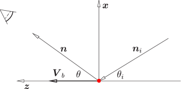
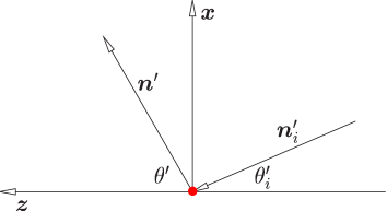
Figure 1: The coordinate system in the (a) lab frame, and (b) rest frame, used to evaluate the polarization matrix. In lab, the clump of electrons indicated at the origin travels along the $z$-axis with velocity $V_{b}$. Note that in the rest frame, we choose to consider the photons scattered in a direction $\bm{n}^{\prime}$ in the $x$-$z$ plane, but the incident photon direction $\bm{n}^{\prime}_{i}$ is in a general direction.

Here we restrict attention to the case where $I_{0}$ is the Planck function at the mean temperature of the CMB, $T_{\rm{CMB}}$:

$$I_{0}(p_{i})=\frac{2c}{h^{2}}\frac{p_{i}^{3}}{e^{p_{i}c/k_{B}T_{\rm{CMB}}}-1}\ .$$ (5)

The incident photon momentum in the lab frame is Doppler shifted on going to the rest frame:

$$p^{\prime}_{i}=\gamma_{b}p_{i}(1-\beta_{b}\mu_{i})\ ,$$ (6)

This may be written in terms of the incident polar angle in the rest frame. Using the formula for relativistic aberration,

$$\mu_{i}=\frac{\mu^{\prime}_{i}+\beta_{b}}{1+\beta_{b}\mu^{\prime}_{i}}\ ,$$ (7)

we obtain

$$p^{\prime}_{i}=\frac{p_{i}}{\gamma_{b}(1+\beta_{b}\mu^{\prime}_{i})}\ .$$ (8)

The specific intensity tensor in the rest frame can be obtained from that in the lab frame using the transformation law of the intensity between frames,

$$I^{\prime}(p^{\prime}_{i},\mu^{\prime}_{i}) = \left(\frac{p^{\prime}_{i}}{p_{i}}\right)^{3}I_{0}(p_{i})=\frac{I_{0}[\gamma_{b}p^{\prime}_{i}(1+\beta_{b}\mu^{\prime}_{i})]}{\gamma_{b}^{3}(1+\beta_{b}\mu^{\prime}_{i})^{3}}$$ (9)

$$= \frac{2h}{c^{2}}\frac{{p^{\prime}_{i}}^{3}}{e^{\gamma_{b}p^{\prime}_{i}(1+\beta_{b}\mu^{\prime}_{i})/k_{B}T_{\rm{CMB}}}-1}\ .$$

The isotropic specific intensity in the lab frame, $I_{0}(p_{i})$, transforms into an anisotropic intensity in the rest frame which is still of blackbody form but with a temperature with angular dependence:

$$T(\mu^{\prime}_{i})=\frac{T_{\rm{CMB}}}{\gamma_{b}(1+\beta_{b}\mu^{\prime}_{i})}\ .$$ (10)

The incident radiation field in the rest frame is of course also unpolarized and has intensity normalized polarization tensor:

$$\bm{I^{\prime}}(\vec{p}_{i},\vec{v}_{e})=I^{\mu^{\prime}\nu^{\prime}}(\vec{p}_{i},\vec{v}_{e})=\frac{1}{2}I^{\prime}(p^{\prime}_{i},\mu^{\prime}_{i})P^{\mu^{\prime}\nu^{\prime}}(\vec{p}_{i},\vec{v}_{e})\ .$$ (11)

In Paper I, the following kinetic equation for the time evolution of the polarization matrix due to Thomson scattering in the electron rest frame was derived (Eqn. (168), Paper I):

$$\frac{d}{dt}I^{\mu\nu}(\vec{p},\vec{v}_{e})=n_{e}\sigma_{\rm T}\Biggl{[}\frac{3}{2}\int\!\frac{d\Omega_{i}}{4\pi}\,P^{\mu}_{\ \ \alpha}(\vec{p},\vec{v}_{e})P^{\nu}_{\ \ \beta}(\vec{p},\vec{v}_{e})I^{\alpha\beta}(\vec{p}_{i},\vec{v}_{e})\Biggr{.}-I^{\mu\nu}(\vec{p},\vec{v}_{e})\Biggr{]}\ ,$$ (12)

where

$$P_{\mu\nu}(\vec{p},\vec{v}\,) = \eta_{\mu\nu}+{1\over p}(p_{\mu}v_{\nu}+p_{\nu}v_{\mu})-{p_{\mu}p_{\nu}\over p^{2}}\quad\quad\mbox{where}\;\;\;p\equiv-v^{\mu}p_{\mu}\ .$$ (13)

Here we have changed the polarization matrix normalization from phase space density to intensity, which is valid in the Thomson limit since the incident and scattered photons have the same energy in the rest frame. The Thomson limit form is appropriate here since even with the boost from the lab to rest frame, the CMB photon momenta are a tiny fraction of the electron mass and therefore recoil is negligible. We evaluate the kinetic equation at photon 4-momentum $\vec{p}$, with the following components in rest frame coordinates:

$$p^{\mu^{\prime}}=p^{\prime}(1,\bm{n}^{\prime}),\;\;\;\bm{n}^{\prime}=\left(\cos\psi^{\prime}\sqrt{1-{\mu^{\prime}}^{2}},\sin\psi^{\prime}\sqrt{1-{\mu^{\prime}}^{2}},\mu^{\prime}\right)\ ,$$ (14)

where $p^{\prime}=p^{\prime}_{i}$ since we are working in the Thomson limit.

In the single scattering limit, we may insert the polarization tensor of the incident unpolarized radiation field in the right hand side of the kinetic equation to obtain the scattered beam:

$$\frac{d}{dt^{\prime}}I^{\mu^{\prime}\nu^{\prime}}(\vec{p},\vec{v}_{e}) = \frac{3}{4}n^{\prime}_{e}\sigma_{T}\int\frac{d\Omega^{\prime}_{i}}{4\pi}I^{\prime}(p^{\prime}_{i},\mu^{\prime}_{i})G^{\mu^{\prime}\nu^{\prime}}(\mu^{\prime},\psi^{\prime};\mu^{\prime}_{i},\psi^{\prime}_{i})-\frac{1}{2}I^{\prime}(p^{\prime},\mu^{\prime})P^{\mu^{\prime}\nu^{\prime}}(\vec{p},\vec{v}_{e})\ ,$$

where

$$G^{\mu^{\prime}\nu^{\prime}}(\mu^{\prime},\psi^{\prime};\mu^{\prime}_{i},\psi^{\prime}_{i}) = P^{\mu^{\prime}}_{\ \ \alpha^{\prime}}(\vec{p},\vec{v}_{e})P^{\nu^{\prime}}_{\ \ \beta^{\prime}}(\vec{p},\vec{v}_{e})P^{\alpha^{\prime}\beta^{\prime}}(\vec{p}_{i},\vec{v}_{e})\ .$$ (16)

The $00$ and $0i$ components of this tensor equation obviously vanish when evaluated in electron rest frame coordinates. We evaluate the gain term by first performing the integral over azimuthal angles $d\psi^{\prime}_{i}$, using the explicit form of the spatial part of the projection tensor:

$$P^{i^{\prime}j^{\prime}}(\vec{p}_{i},\vec{v}_{e})=\left(\begin{array}[]{ccc}1+({\mu^{\prime}_{i}}^{2}-1)\cos^{2}\psi^{\prime}_{i}&({\mu^{\prime}_{i}}^{2}-1)\cos\psi^{\prime}_{i}\sin\psi^{\prime}_{i}&-\mu^{\prime}_{i}\sqrt{1-{\mu^{\prime}_{i}}^{2}}\cos\psi^{\prime}_{i}\\ ({\mu^{\prime}_{i}}^{2}-1)\cos\psi^{\prime}_{i}\sin\psi^{\prime}_{i}&1+({\mu^{\prime}_{i}}^{2}-1)\sin^{2}\psi^{\prime}_{i}&-\mu^{\prime}_{i}\sqrt{1-{\mu^{\prime}_{i}}^{2}}\sin\psi^{\prime}_{i}\\ -\mu^{\prime}_{i}\sqrt{1-{\mu^{\prime}_{i}}^{2}}\cos\psi^{\prime}_{i}&-\mu^{\prime}_{i}\sqrt{1-{\mu^{\prime}_{i}}^{2}}\sin\psi^{\prime}_{i}&1-{\mu^{\prime}_{i}}^{2}\end{array}\right)\ .$$ (20)

Performing the integral over azimuth yields

$$\int_{0}^{2\pi}\frac{d\psi^{\prime}_{i}}{2\pi}P^{i^{\prime}j^{\prime}}(\vec{p}_{i},\vec{v}_{e})=\left(\begin{array}[]{ccc}\frac{1}{2}(1+{\mu^{\prime}_{i}}^{2})&0&0\\ 0&\frac{1}{2}(1+{\mu^{\prime}_{i}}^{2})&0\\ 0&0&\frac{1}{2}(1-{\mu^{\prime}_{i}}^{2})\end{array}\right)\ .$$ (24)

To further simplify, we may evaluate the rest of the scattering term at $\psi^{\prime}=0$, since by azimuthal symmetry of the radiation field in the rest frame the intensity tensor for a general $(\mu^{\prime},\psi^{\prime})$ is related to that at $\psi^{\prime}=0$ by a rotation about the $z$–axis through angle $\psi^{\prime}$, and the polarization magnitude is independent of azimuth. Putting $\bm{n}^{\prime}=\left(\sqrt{1-{\mu^{\prime}}^{2}},0,\mu^{\prime}\right)$, the explicit form of the spatial part of the projection tensor is $P^{i^{\prime}j^{\prime}}(\vec{p},\vec{v}_{e})$ is:

$$P^{i^{\prime}j^{\prime}}(\vec{p},\vec{v}_{e})=\left(\begin{array}[]{ccc}{\mu^{\prime}}^{2}&0&-\mu^{\prime}\sqrt{1-{\mu^{\prime}}^{2}}\\ 0&1&0\\ -\mu^{\prime}\sqrt{1-{\mu^{\prime}}^{2}}&0&1-{\mu^{\prime}}^{2}\end{array}\right)\ .$$ (28)

Now performing the multiplication of two of the matrices in Eqn. (28) with the matrix in Eqn. (24), yields the azimuthal integral of Eqn. (16) required in the gain term of the kinetic equation (I):

$$\bar{G}^{i^{\prime}j^{\prime}}\equiv\int_{0}^{2\pi}\frac{d\psi^{\prime}_{i}}{2\pi}\;G^{i^{\prime}j^{\prime}}(\mu^{\prime},0;\mu^{\prime}_{i},\psi^{\prime}_{i})\;=$$

$$\quad\quad\frac{1}{2}\left(\begin{array}[]{ccc}G_{\parallel}(\mu^{\prime},\mu^{\prime}_{i}){\mu^{\prime}}^{2}&0&-\mu^{\prime}\sqrt{1-{\mu^{\prime}}^{2}}G_{\parallel}(\mu^{\prime},\mu^{\prime}_{i})\\ 0&G_{\perp}(\mu^{\prime},\mu^{\prime}_{i})&0\\ -\mu^{\prime}\sqrt{1-{\mu^{\prime}}^{2}}G_{\parallel}(\mu^{\prime},\mu^{\prime}_{i})&0&G_{\parallel}(\mu^{\prime},\mu^{\prime}_{i})\left(1-{\mu^{\prime}}^{2}\right)\end{array}\right)\ ,\quad\quad\quad\quad$$ (32)

where

$$G_{\parallel}(\mu^{\prime},\mu^{\prime}_{i}) = 2-{\mu^{\prime}}^{2}+{\mu^{\prime}_{i}}^{2}\left(3{\mu^{\prime}}^{2}-2\right)\ ,$$

$$G_{\perp}(\mu^{\prime},\mu^{\prime}_{i}) = 1+{\mu^{\prime}_{i}}^{2}\ .$$ (33)

One can check that

$$\frac{1}{2}\int_{-1}^{1}d\mu^{\prime}_{i}\;\bar{G}^{\mu^{\prime}\nu^{\prime}}=\frac{2}{3}P^{\mu^{\prime}\nu^{\prime}}(\vec{p},\vec{v}_{e})\ ,$$ (34)

(evaluated at $\psi^{\prime}=0$). Thus as $\beta_{b}\to 0$, $\frac{d}{dt}I^{\mu^{\prime}\nu^{\prime}}(\vec{p},\vec{v}_{e})\to 0$, since by symmetry scattering of an isotropic radiation field from a stationary electron cannot alter the radiation field.

Now putting together the gain and loss terms, and integrating $\mu^{\prime}_{i}$, we find for a finite rest frame time interval $\Delta t^{\prime}$ (all evaluated at $\psi^{\prime}=0$ in rest frame coordinates):

$$\frac{\bm{\Delta I^{\prime}}(\vec{p},\vec{v}_{e})}{\tau_{\rm T}^{\prime}}=\frac{1}{2}\left(\begin{array}[]{ccc}I_{\parallel}(p^{\prime},\mu^{\prime}){\mu^{\prime}}^{2}&0&-\mu^{\prime}\sqrt{1-{\mu^{\prime}}^{2}}I_{\parallel}(p^{\prime},\mu^{\prime})\\ 0&I_{\perp}(p^{\prime},\mu^{\prime})&0\\ -\mu^{\prime}\sqrt{1-{\mu^{\prime}}^{2}}I_{\parallel}(p^{\prime},\mu^{\prime})&0&I_{\parallel}(p^{\prime},\mu^{\prime})\left(1-{\mu^{\prime}}^{2}\right)\end{array}\right)\ ,\quad\quad$$ (35)

where we set the optical depth in the rest frame to $\tau_{\rm T}^{\prime}\equiv n^{\prime}_{e}\sigma_{T}\Delta t^{\prime}$, and defined

$$I_{\parallel}(p^{\prime},\mu^{\prime}) = \frac{3}{8}\left[(2-\mu^{\prime 2})J(p^{\prime})+(3\mu^{\prime 2}-2)K(p^{\prime})-\frac{8}{3}I^{\prime}(p^{\prime},\mu^{\prime})\right]\ ,$$

$$I_{\perp}(p^{\prime},\mu^{\prime}) = \frac{3}{8}\left[J(p^{\prime})+K(p^{\prime})-\frac{8}{3}I^{\prime}(p^{\prime},\mu^{\prime})\right]\ ,$$ (36)

and the functions (note that these are functions of $p^{\prime}_{i}$, but in the Thomson limit this equals the scattered photon momentum $p^{\prime}$):

$$J(p^{\prime}) \equiv \int_{-1}^{1}d\mu^{\prime}_{i}\;I^{\prime}(p^{\prime},\mu^{\prime}_{i})\ ,$$

$$K(p^{\prime}) \equiv \int_{-1}^{1}d\mu^{\prime}_{i}\;I^{\prime}(p^{\prime},\mu^{\prime}_{i}){\mu^{\prime}_{i}}^{2}\ .$$ (37)

Using the dimensionless frequency $x^{\prime}=cp^{\prime}/k_{B}T_{\rm{CMB}}$, and the constant $i_{0}=2(k_{B}T_{\rm{CMB}})^{3}/(hc)^{2}$, these functions are given by the integrals

$$J(x^{\prime},\beta_{b}) = i_{0}x^{\prime 3}\int_{-1}^{1}d\mu^{\prime}_{i}\left[e^{\gamma_{b}x^{\prime}(1+\beta_{b}\mu^{\prime}_{i})}-1\right]^{-1}\ ,$$

$$K(x^{\prime},\beta_{b}) = i_{0}x^{\prime 3}\int_{-1}^{1}{\mu^{\prime}_{i}}^{2}d\mu^{\prime}_{i}\left[e^{\gamma_{b}x^{\prime}(1+\beta_{b}\mu^{\prime}_{i})}-1\right]^{-1}\ .$$ (38)

The intensity of the scattered radiation in the lab frame is thus given by the trace

$$\Delta I^{\prime}(x^{\prime},\mu^{\prime}) = \mbox{Tr}[\bm{\Delta I^{\prime}}(\vec{p},\vec{v}_{e})]$$ (39)

$$= \frac{3}{16}\tau_{\rm T}^{\prime}\left[(3-\mu^{\prime 2})J(x^{\prime},\beta_{b})+(3\mu^{\prime 2}-1)K(x^{\prime},\beta_{b})-\frac{16}{3}I^{\prime}(x^{\prime},\mu^{\prime})\right]\!\!\quad\quad\quad$$

where

$$I^{\prime}(x^{\prime},\mu^{\prime})=i_{0}x^{\prime 3}\left[e^{\gamma_{b}x^{\prime}(1+\beta_{b}\mu^{\prime})}-1\right]^{-1}\ .$$ (40)

The polarization magnitude, in the limit of small $\tau_{\rm T}^{\prime}$ is given by the formula for the polarization of a perturbed unpolarized beam, given in Eqn. (52) of Paper I:

$$\Pi(x^{\prime},\mu^{\prime})=\Pi(\bm{I^{\prime}}(\vec{p},\vec{v}_{e})+\bm{\Delta I^{\prime}}(\vec{p},\vec{v}_{e}))=\left(\frac{\mbox{Tr}[\bm{\Delta I^{\prime}}]}{\mbox{Tr}[\bm{I^{\prime}}]}\right)\Pi(\bm{\Delta I^{\prime}})\ ,$$ (41)

where

$$\Pi^{2}(\bm{\Delta I^{\prime}})=\frac{2\mbox{Tr}[\bm{\Delta I^{\prime}}^{2}]}{\mbox{Tr}[\bm{\Delta I^{\prime}}]^{2}}-1\ .$$ (42)

Evaluating this, we find

$$\Pi(x^{\prime},\mu^{\prime})=\frac{3}{16}\tau_{\rm T}^{\prime}\;\left(1-\mu^{\prime 2}\right)\;\frac{3K(x^{\prime},\beta_{b})-J(x^{\prime},\beta_{b})}{I^{\prime}(x^{\prime},\mu^{\prime})}\ .$$ (43)

This formula, and the $\mu^{\prime}_{i}$ angular dependence inside the integrands of $K$ and $J$, shows that only the quadrupole in the incident intensity in the rest frame generates polarization. The polarization magnitude has the familiar $\sin^{2}\theta^{\prime}$ dependence. As $\beta_{b}\rightarrow 0$, the incident radiation field in the rest frame becomes isotropic, $I^{\prime}(x^{\prime},\mu^{\prime})\rightarrow I_{0}$ (of Eqn. (5)), yielding $J\rightarrow 2I_{0},K\rightarrow 2I_{0}/3$, and thus $\Pi(x^{\prime},\mu^{\prime})\rightarrow 0$ as expected.

We now expand the integrands of $J(x^{\prime},\beta_{b})$ and $K(x^{\prime},\beta_{b})$ in powers of $\beta_{b}$:

$$\left[e^{\gamma_{b}x^{\prime}(1+\beta_{b}\mu^{\prime})}-1\right]^{-1}=n_{0}(x)-\frac{e^{x^{\prime}}}{(e^{x^{\prime}}-1)^{2}}\sum_{n=0}^{\infty}\left(\frac{e^{x^{\prime}}}{e^{x^{\prime}}-1}\right)^{n}(-1)^{n}\delta^{n+1}\ ,$$ (44)

where

$$\delta\equiv e^{(\gamma_{b}-1)x^{\prime}}e^{\gamma_{b}\beta_{b}\mu^{\prime}x^{\prime}}-1\ .$$ (45)

Expanding $\delta$ up to second order in $\beta_{b}$, we find:

$$\int_{-1}^{1}d\mu^{\prime}\;\delta = \beta_{b}^{2}x^{\prime}\left(1+\frac{1}{3}x^{\prime}\right)+O(\beta_{b}^{4})\ ,$$

$$\int_{-1}^{1}d\mu^{\prime}\;\delta^{2} = \frac{2}{3}\beta_{b}^{2}x^{\prime 2}+O(\beta_{b}^{4})\ ,$$

$$\int_{-1}^{1}d\mu^{\prime}\;\mu^{\prime 2}\;\delta = \frac{1}{3}\beta_{b}^{2}x^{\prime}\left(1+\frac{3}{5}x^{\prime}\right)+O(\beta_{b}^{4})\ ,$$

$$\int_{-1}^{1}d\mu^{\prime}\;\mu^{\prime 2}\;\delta^{2} = \frac{2}{5}\beta_{b}^{2}x^{\prime 2}+O(\beta_{b}^{4})\ .$$ (46)

To obtain $\Pi(x^{\prime},\mu^{\prime})$ to second order in $\beta_{b}$, since the numerator is already second order, we may replace $I^{\prime}(x^{\prime},\mu^{\prime})$ in Eqn. (43) with $I_{0}$.

Using the results in the previous equation we obtain finally the polarization magnitude in the rest frame to second order in $\beta_{b}$:

$$\Pi(x^{\prime},\mu^{\prime})=\frac{1}{20}\;\tau_{\rm T}^{\prime}x^{\prime 2}\frac{e^{x^{\prime}}(e^{x^{\prime}}+1)}{(e^{x^{\prime}}-1)^{2}}\beta_{b}^{2}\;(1-\mu^{\prime 2})\ .$$ (47)

On Lorentz transforming into the lab frame, the polarization magnitude of the scattered photons does not change, but the photon angle is aberrated, with

$$\mu^{\prime}=\frac{\mu-\beta_{b}}{1-\beta_{b}\mu}\ .$$ (48)

Since $\mu^{\prime 2}=\mu^{2}+O(\beta_{b})$, and $x^{\prime}=x+O(\beta_{b})$, and the optical depth $\tau^{\prime}_{\rm T}$ transforms like $dt^{\prime}$, we have the same result in the lab frame quantities to this order:

$$\Pi(x,\mu)=\frac{1}{20}\;\tau_{\rm T}x^{2}\frac{e^{x}(e^{x}+1)}{(e^{x}-1)^{2}}\beta_{b}^{2}\;(1-\mu^{2})\ .$$ (49)

 

(a)   Dimensionless $\Pi/\tau_{\rm T}$

(b)   Brightness temperature $\Pi$

Figure 2: Polarization magnitude of the CMB scattered by a concentrated cloud of cold electrons with a bulk flow velocity $V_{b}$ transverse to the line of sight. In (a), we plot the dimensionless polarization magnitude $\Pi(x)$ divided through by the optical depth $\tau_{\rm T}$. In (b), we plot the polarization magnitude $\Pi(x)$ as a (Rayleigh-Jeans) brightness temperature distortion, taking $\tau_{\rm T}=0.01$. The upper and lower curves in both (a) and (b) correspond to $V_{b}=5000\;\mbox{km s}^{-1}$ and $V_{b}=1000\;\mbox{km s}^{-1}$ respectively.

This result was obtained before by Sazonov & Sunyaev (1999); Audit & Simmons (1999); Challinor et al. (2000), all using different methods. Note that the $(1-\mu^{2})$ dependence implies that this component of the CMB polarization is a direct measure of the peculiar velocity of the cluster gas perpendicular to the line of sight, which in conjunction with the intensity measurement allows, in principle, measurement of all the components of the cluster peculiar velocity. This will be an important cosmological probe, if the polarization measurements can be made. This will be a considerable experimental challenge, since the polarization magnitude is rather small, typically $0.1\,\mu\mbox{K}$ at most, as illustrated in Fig. 2 (note that cluster bulk velocities rarely exceed $1000\,\mbox{km \!s}^{-1}$). In panel (b) we show the polarization magnitude as a Rayleigh-Jeans (RJ) brightness temperature, given by

$$\Delta T_{B}=\frac{T_{\rm{CMB}}}{i_{0}x^{2}}\sqrt{\Delta Q^{2}_{\nu}+\Delta U^{2}_{\nu}}\ .$$ (50)

One might worry that the dimensionless polarization magnitude $\Pi$ goes quadratically in $x$ as $x\rightarrow\infty$, which would seem to be a problem since the polarization magnitude must be bounded by unity. However, the analysis we have given is only the lowest order result - at high photon frequencies, relativistic corrections will modify Eqn. (49). Since we essentially expanded in powers of $\beta_{b}x$, our analysis cannot be trusted for frequencies greater than $x\approx 1/\beta_{b}$.

We finish this section by expanding the total intensity of the scattered radiation, given in Eqn. (39), to second order in $\beta_{b}$, and performing the transformation to lab frame to obtain the kinematic SZ distortion and its first relativistic correction. To do this calculation it is convenient to work with the phase space density rather than the intensity. The intensity distortion $\Delta I^{\prime}(x^{\prime},\mu^{\prime})$ is related to the phase space density distortion by

$$\frac{\Delta I^{\prime}(x^{\prime},\mu^{\prime})}{I^{\prime}(x^{\prime},\mu^{\prime})}=\frac{\Delta f^{\prime}(x^{\prime},\mu^{\prime})}{f^{\prime}(x^{\prime},\mu^{\prime})}\ .$$ (51)

From the transformation law of the left hand side of the kinetic equation, given by Eqn. (204) of Paper I, we find an equation for the rate of change of the phase space density in lab:

$$\frac{1}{f(x,\mu)}\frac{df(x,\mu)}{dt}=\gamma_{b}(1-\beta_{b}\mu)\;n^{\prime}_{e}\sigma_{\rm T}\left(\frac{\Delta I^{\prime}(x^{\prime},\mu^{\prime})}{\tau_{\rm T}^{\prime}I^{\prime}(x^{\prime},\mu^{\prime})}\right)\ .$$ (52)

Expanding the functions $K(x^{\prime},\beta_{b})$ and $J(x^{\prime},\beta_{b})$ in Eqn. (39) up to second order in $\beta_{b}$ as before, and expressing the right hand side in lab frame quantities by making the replacements $x^{\prime}=\gamma_{b}x(1-\beta_{b}\mu)$, $\mu^{\prime}=(\mu-\beta_{b})/(1-\beta_{b}\mu)$ and $n^{\prime}_{e}=n_{e}/\gamma_{b}$, we find to $O(\beta_{b}^{2})$ the fractional intensity distortion in lab:

$$\frac{\Delta I(x,\mu)}{I_{0}(x)}=\tau_{\rm T}\frac{xe^{x}}{e^{x}-1}\left[\mu\,\beta_{b}+\left(-1-{\mu}^{2}+\frac{x\left(3+11\,{\mu}^{2}\right)\,\coth(\frac{x}{2})}{20}\right)\,{\beta_{b}}^{2}\right]\ ,$$ (53)

where the lab frame optical depth is defined by $\tau_{\rm T}=n_{e}\sigma_{\rm T}\Delta t$. This is the first relativistic correction to the kinematic SZ effect, obtained previously by Sazonov & Sunyaev (1998a, b). Note that without the correct “flux factor” $\gamma_{b}(1-\beta_{b}\mu)$ in Eqn. (52), this would differ at second order in $\beta_{b}^{2}$. The first term is simply the lowest order kinematic SZ distortion, where $V_{r}=-\mu\beta_{b}$ is the bulk velocity projected along the line of sight (which is opposite to the direction of the scattered photon momentum, hence the minus sign).

II Hot electrons

We now extend to the more general case of a Maxwellian distribution of electrons with dimensionless temperature $\theta_{e}\equiv k_{B}T_{e}/m_{e}$ moving with a bulk velocity $\bm{V}_{b}$ with respect to the CMB rest frame (lab frame). In the single scattering limit, the Thomson scattering of isotropic blackbody radiation from a Maxwellian distribution of electrons moving with a bulk velocity $\bm{V}_{b}=\bm{\beta}_{b}c$ produces a scattered radiation field whose intensity and polarization magnitude are azimuthally symmetric about $\bm{V}_{b}$. Our goal is to compute the polarization matrix of the scattered radiation field, as an expansion in powers of $V_{b}$ and $\theta$. This computation will yield, to lowest order, the usual thermal and kinematic SZ distortion of the intensity, and the polarization magnitude to lowest order in $V_{b}$. Going to higher order yields the “interference” terms between the thermal and kinematic effects, in both the intensity and polarization, and the relativistic corrections.

The first task is to determine the lab frame polarization matrix of the scattered beam due to scattering of an incident unpolarized isotropic blackbody radiation field in lab by an electron with a general lab frame velocity $\bm{\beta}$. This is not the bulk velocity but rather the velocity of some of the electrons in the thermal distribution, which will eventually be integrated over. This part is just a generalization of the calculation performed in section §I. The resulting polarization matrix of the lab frame scattered radiation field as a function of electron velocity may then be averaged over a distribution of lab frame electron velocities to yield the observed lab frame result. The steps required to compute this are described below. The actual calculation, even at lowest order, is quite lengthy, so a computer algebra system (Mathematica (Wolfram, 1991)) was used to perform the calculation. We do not give all the algebra but just outline the procedure. Henceforth in this section primed indices refer to components of 4-vectors in the electron rest frame, and unprimed indices to components in the lab frame.

It is convenient to integrate over angles in the electron rest frame, but to express the electron velocity and final state photon momentum in lab coordinates throughout (to avoid a cumbersome transformation of rest frame angles to lab frame). In lab frame coordinates, the electron 4-velocity is

$$v^{\mu}_{e}=\gamma(1,\bm{\beta})\ ,\quad\gamma\equiv\frac{1}{\sqrt{1-\beta^{2}}}\ ,\quad\beta\equiv|\bm{\beta}|\ .$$ (54)

The Cartesian coefficients of $\bm{\beta}$ are denoted $\beta_{i}$. In rest frame coordinates, the velocity of the lab frame is of course

$$v^{\mu^{\prime}}_{l}=\gamma(1,-\bm{\beta})\ .$$ (55)

The scattered photon momentum in lab frame coordinates is written

$$p^{\mu}_{s}=p_{s}(1,\bm{n}_{s})\ .$$ (56)

To simplify the computation, we set up a polar coordinate system with polar axis along the $z$-direction and evaluate the scattered polarization matrix at azimuth $\psi_{s}=0$:

$$\bm{n}_{s} = \left(\sqrt{1-\mu_{s}^{2}},\;0,\;\mu_{s}\right)\ .$$ (57)

This is no loss of generality provided we choose the bulk velocity $\bm{V}_{b}$ to lie along the $z$–direction, in which case the polarization matrix for a general $\bm{n}_{s}$ is related to the one calculated here by a simple rotation about the $z$–axis.

The scattered photon momentum in the electron rest frame is found by applying Lorentz transformation matrices to obtain $p_{s}^{\mu^{\prime}}=\Lambda^{\mu^{\prime}}_{\;\;\;\mu}(\bm{\beta})\;p_{s}^{\mu}$, where

$$\Lambda^{0}_{\;\;\;0} = \gamma=1/\sqrt{1-\beta^{2}},\quad\quad\Lambda^{0}_{\;\;\;i}=\Lambda^{i}_{\;\;\;0}=-\gamma\beta^{i}\ ,$$

$$\Lambda^{i}_{\;\;\;j} = (\gamma-1)\frac{\beta^{i}\beta_{j}}{\beta^{2}}+\delta^{i}_{\;\;\;j}\ .$$ (58)

Using the notation of §LABEL:ch3:sec3, we denote the momenta of the incident photons in the lab and rest frames as follows:

$$p^{\mu}_{i} = p_{i}(1,\bm{n}_{i})\ ,\quad p^{\mu^{\prime}}_{i}=p^{\prime}_{i}(1,\bm{n}^{\prime}_{i})\ ,$$

$$\bm{n}^{\prime}_{i} = \left(\cos\psi^{\prime}_{i}\sqrt{1-{\mu^{\prime}_{i}}^{2}},\;\sin\psi^{\prime}_{i}\sqrt{1-{\mu^{\prime}_{i}}^{2}},\;\mu^{\prime}_{i}\right)\ .$$ (59)

with $p_{i}=-\vec{v}_{l}\cdot\vec{p}_{i}$, $p^{\prime}_{i}=-\vec{v}_{e}\cdot\vec{p}_{i}$. In the lab frame, the scalar occupation number of the incident photons is isotropic with a Planck spectrum:

$$n_{i}(\vec{p}_{i})=\frac{1}{e^{p_{i}/k_{B}T_{\rm CMB}}-1}\ .$$ (60)

(Note, do not confuse $\bm{n}_{i}$, a direction vector, with $n_{i}$, the occupation number!). In the rest frame, $n^{\prime}_{i}(\vec{p}_{i})=n_{i}(\vec{p}_{i})$, but the occupation number of the incident photons is no longer isotropic since photons with different momenta are aberrated through different angles. Thus $n_{i}$ becomes a function of $p^{\prime}_{i}$ and $\bm{n}^{\prime}_{i}$ through $p_{i}$:

$$n^{\prime}_{i}(\vec{p}_{i})=\frac{1}{e^{p_{i}(p^{\prime}_{i},\bm{n}^{\prime}_{i})/k_{B}T_{\rm CMB}}-1}\ ,$$ (61)

where in terms of $\bm{\beta}$,

$$p_{i}(p^{\prime}_{i},\bm{n}^{\prime}_{i})=\gamma p^{\prime}_{i}\left(1+\bm{\beta}\cdot\bm{n}^{\prime}_{i}\right)\ .$$ (62)

The angular dependence of the incident radiation field in the rest frame is obtained by expanding (61) in powers of the velocity components $\beta_{i}$. For the lowest order polarization computation, the expansion must be taken up to at least second order in the velocity components.

Then as in the previous section, the right hand side of the rest frame master equation (12) is constructed, and the integration over the rest frame angles of the incident beam performed. The resulting matrix is then transformed into lab frame by the application of two projection tensors, and the lab frame fractional intensity distortion obtained, making sure, as in Eqn. (52), to multiply by the correct flux factor, which now has the form $\gamma(1-\bm{\beta}\cdot\bm{n})$.

We thus obtain the lab frame polarization matrix as a function of the lab frame photon direction and the velocity components $\bm{\beta}$. In the lab frame, the integration over electron velocities is performed. To do this we need first to construct the distribution function of electron velocities in lab frame. In the “comoving frame”, denoted with primes, in which the average electron velocity vanishes, the electron phase space distribution function as a function of the electron 3-momentum $\bm{q}^{\prime}$ is assumed to be a relativistic Maxwellian at dimensionless temperature $\theta_{e}$:

$$g_{e}(\bm{q}^{\prime})=g_{0}\,e^{-E(\bm{q}^{\prime})/(m_{e}\theta_{e})}\ .$$ (63)

where $E(\bm{q}^{\prime})=\sqrt{\bm{q}^{\prime 2}+m_{e}^{2}}$, and $g_{0}$ is a normalization constant which depends on the total number density of electrons. We use a relativistic Maxwellian in order to retain the corrections to the SZ effect in a mildly relativistic plasma.

With $\bm{q}^{\prime}=m_{e}\gamma^{\prime}\bm{\beta}^{\prime}$, where $\bm{\beta}^{\prime}$ is the electron 3-velocity in the comoving frame, and $\gamma^{\prime}\equiv 1/\sqrt{1-\beta^{\prime 2}}$, we have (as a function of $\beta$ since the distribution is isotropic in the comoving frame)

$$g_{e}(\beta^{\prime})=g_{0}\,e^{-\gamma^{\prime}/\theta_{e}}\ .$$ (64)

The number density of electrons in each comoving frame momentum element $d^{3}p^{\prime}$ is thus

$$dn^{\prime}_{e}=4\pi g_{0}\,p^{\prime 2}\;dp^{\prime}e^{-\gamma^{\prime}/\theta_{e}}\ .$$ (65)

Integrating this distribution over the element $d^{3}p^{\prime}$ yields the electron number density in the comoving frame $n^{\prime}_{e}$. Using $p^{\prime}=m_{e}\gamma^{\prime}\beta^{\prime}$, we find $p^{\prime 2}dp^{\prime}=m_{e}^{3}\gamma^{\prime 5}\beta^{\prime 2}d\beta^{\prime}$. Thus

$$n^{\prime}_{e} = g_{0}\int 4\pi\gamma^{\prime 5}\beta^{\prime 2}d\beta^{\prime}e^{-\gamma^{\prime}/\theta_{e}}$$ (66)

$$= 4\pi g_{0}\,m_{e}^{3}\;\theta_{e}K_{2}(1/\theta_{e})\ ,$$

where $K_{2}$ is a modified Bessel function (for a derivation of this result see for example Synge (1957)).

Thus in the comoving frame, the number density of electrons in each comoving frame velocity element $d^{3}v^{\prime}$, is

$$dn^{\prime}_{e} = n^{\prime}_{e}\frac{d^{3}\beta^{\prime}}{4\pi}\frac{\gamma^{\prime 5}e^{-\gamma^{\prime}/\theta_{e}}}{\theta_{e}K_{2}(1/\theta_{e})}\ .$$ (67)

For small $\theta_{e}$, the denominator can be expanded:

$$4\pi\theta_{e}K_{2}(1/\theta_{e})e^{1/\theta_{e}}=(2\pi\theta_{e})^{3/2}\left[1+15\theta_{e}/8+\cdots\right]\ ,$$ (68)

yielding the familiar prefactor of the non-relativistic Maxwellian to lowest order.

Now we wish to compute the analogous lab frame quantity by a Lorentz transformation from the comoving frame. Since the distribution function is a Lorentz scalar, the number density element transforms like the momentum space volume element in Eqn. (65). Using the Lorentz invariance of the quantity $d^{3}p/p=d^{3}p^{\prime}/p^{\prime}$, it follows that

$$p^{\prime 2}dp^{\prime}=m_{e}^{3}\gamma^{\prime 5}\beta^{\prime 2}d\beta^{\prime}=m_{e}^{3}\gamma^{5}\beta^{2}d\beta(\gamma^{\prime}/\gamma)\ .$$ (69)

Choosing the bulk velocity of the comoving frame with respect to the lab frame to be $V_{b}=\beta_{b}c$ in the $z$-direction, we have

$$\gamma^{\prime}/\gamma=\gamma_{b}\left(1-\beta_{z}\beta_{b}\right)\ ,\quad\quad\gamma_{b}\equiv(1-\beta_{b}^{2})^{-1/2}\ .$$ (70)

For calculations it is convenient to write the distribution function in lab frame in a form in which the non-relativistic part of the Maxwellian, which has Gaussian form, is pulled out and the rest expanded in a series in powers of the velocity relative to the dimensionless bulk velocity $\bm{\beta}_{b}=(0,0,\beta_{b})$:

$$\frac{dn_{e}}{n_{e}}=\frac{e^{-(\gamma-1)/\theta_{e}}}{\theta_{e}e^{1/\theta_{e}}K_{2}(1/\theta_{e})}\left[\gamma^{5}\gamma_{b}\left(1-\beta_{z}\beta_{b}\right)e^{-\gamma\left[\gamma_{b}(1-\beta_{z}\beta_{b})-1\right]/\theta_{e}}\right]\frac{d^{3}\bm{\beta}}{4\pi}\ .$$ (71)

Making the substitution $\beta_{z}\rightarrow\tilde{\beta}_{z}+V_{b}$, the part in square brackets may be expanded straightforwardly about unity in powers of $\beta_{x},\beta_{y},\tilde{\beta}_{z}$, $\beta_{b}$ and $\theta_{e}$. Defining

$$\tilde{\beta}^{2}\equiv\beta_{x}^{2}+\beta_{y}^{2}+\tilde{\beta}_{z}^{2}\ ,$$ (72)

the exponential factor in front can be written as

$$e^{-\tilde{\beta}^{2}/2\theta_{e}}\times\mbox{prefactor}\ ,$$ (73)

where the prefactor is an expansion about unity in powers of $\tilde{\beta_{z}},\beta_{x},\beta_{y}$. The result is a Gaussian multiplied by a prefactor which is polynomial in the components $\beta_{i}$ with coefficients which are functions of $\beta_{b}$ and $\theta_{e}$.

A further transformation is required before the lab frame integral can be done. The integral $d^{3}\bm{\beta}$ ranges over the velocity sphere $|\bm{\beta}|\leq 1$. To simplify the Gaussian integrals, it is easier to make the transformation $\beta_{i}\rightarrow u_{i}/\gamma$, and integrate $d^{3}\bm{u}$ over all space. With this transformation, we find

$$\gamma=\sqrt{1+u^{2}}\ ,\quad\quad\gamma^{5}\beta^{2}d\beta=u^{2}du\ .$$ (74)

Steps similar to those described above yield an expansion about the transformed bulk velocity $\bm{\beta}_{b}\rightarrow\bm{U}_{b}=(0,0,\beta_{b}/\sqrt{1+\beta_{b}^{2}})$ in powers of $\tilde{u}_{z}=u_{z}-\beta_{b}/\sqrt{1-\beta_{b}^{2}}$, $u_{x},u_{y}$. This form is then convenient for integration by a symbolic algebra package.

We expand the prefactor to terms up to sixth order in the coefficients, and up to second order in both $\beta_{b}$ and $\theta_{e}$. Integration over the electron distribution function then yields the lab frame polarization matrix as a function of the bulk velocity $\beta_{b}$ and electron temperature $\theta_{e}$. Taking the trace of this matrix gave the following result for the intensity distortion:

 

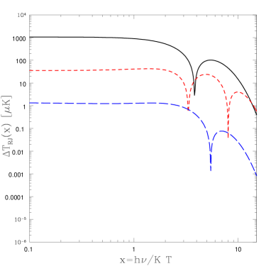
(a)   Thermal effect

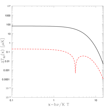
(b)   Kinematic effect

Figure 3: The frequency dependence of the thermal and kinematic SZ effects and their first relativistic corrections (as RJ brightness temperature distortions, as defined in Eqn. (50)). The solid lines in each plot show the lowest order effect, and the short dashed lines show the first relativistic correction. The long dashed line in plot (a) shows the “interference” term $F_{1}^{TK}$.

$$\frac{\Delta I}{I_{0}} = \tau_{\rm T}\frac{xe^{x}}{e^{x}-1}\left[\theta_{e}F^{T}_{0}(x)+\theta^{2}_{e}F^{T}_{1}(x)\right.$$ (75)

$$\left.\quad\quad\quad+\,\beta_{b}F^{K}_{0}(\mu)+\beta_{b}^{2}F^{K}_{1}(x,\mu)+\theta_{e}\beta_{b}F^{TK}_{1}(x,\mu)+\cdots\right]\ .$$

Here $F^{T}_{0}$ is the well known thermal SZ distortion piece, and $F^{T}_{1}$ is the first relativistic correction to the thermal effect:

$$F^{T}_{0}(x) = -4+x\,\coth\left(\frac{x}{2}\right)$$

$$F^{T}_{1}(x) = e^{\frac{3\,x}{2}}\,\left[5\,{\left(-1+e^{x}\right)}^{3}\right]^{-1}\left[x\,\left(-235+77\,x^{2}\right)\,\cosh\left(\frac{x}{2}\right)\right.$$ (76)

$$\left.+x\,\left(235+7\,x^{2}\right)\,\cosh\left(\frac{3\,x}{2}\right)\right.$$

$$\left.-8\,\left(-25+42\,x^{2}+\left(25+21\,x^{2}\right)\,\cosh(x)\right)\,\sinh\left(\frac{x}{2}\right)\right]\ .$$

The frequency dependence obtained here agrees with that obtained by Sazonov & Sunyaev (1998a, b); Itoh et al. (2000); Challinor et al. (2000).

The terms $F_{0}^{K}$ and $F_{1}^{K}$ are the lowest order kinematic effect and the first relativistic correction respectively:

$$F^{K}_{0}(\mu) = \mu\ ,$$

$$F^{K}_{1}(x,\mu) = -1-{\mu}^{2}+\frac{x\left(3+11\,{\mu}^{2}\right)\,\coth(\frac{x}{2})}{20}\ .$$ (77)

which agree with the forms in Sazonov & Sunyaev (1998a, b); Itoh et al. (2000); Challinor et al. (2000). The “interference” term between the thermal and kinematic effects is:

$$F^{TK}_{1}(x,\mu) = \mu\,\frac{\left[-45+14\,x^{2}+\left(45+7\,x^{2}\right)\,\cosh(x)-47\,x\,\sinh(x)\right]}{10\;{\sinh^{2}\left(x/2\right)}}\,\ .$$ (78)

The thermal and kinematic effects, their relativistic corrections, and the interference term are plotted for representative cluster parameters in Fig. 3. These were computed for a cluster with electrons at temperature $k_{B}T_{e}=10$ keV, a bulk flow velocity $V_{b}=1000\;\mbox{km s}^{-1}$ at an angle cosine $\mu=1/\sqrt{2}$ to the line of sight, and an optical depth to scattering of $\tau_{\rm T}=0.01$. (Note that the dips in the curves are zero crossings).

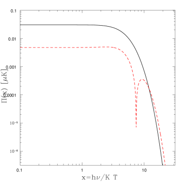
Figure 4: Polarization magnitude generated by scattering of CMB monopole (solid line), and the first relativistic correction (dashed line), as RJ brightness temperature distortions, in the case of a concentrated cluster with electrons at temperature $k_{B}T_{e}=10$ keV, a bulk flow velocity $V_{b}=1000\;\mbox{km s}^{-1}$ perpendicular to the line of sight, and an optical depth to scattering of $\tau_{\rm T}=0.01$.

Computing the polarization magnitude of the final lab frame matrix, we find:

$$\Pi(x,\mu) = \tau_{\rm T}\;\beta_{b}^{2}\,\left(1-{\mu}^{2}\right)\left[F^{P}_{0}(x)+F^{P}_{1}(x)\theta_{e}+O(\theta_{e}^{2})\right]\ ,$$ (79)

where

$$F^{P}_{0}(x) = \frac{e^{x}\,\left(1+e^{x}\right)\,x^{2}\,}{20\,{\left(-1+e^{x}\right)}^{2}}\ ,$$ (80)

and

$$F^{P}_{1}(x) = \frac{e^{\frac{5\,x}{2}}\,x^{2}\,}{10\,{\left(-1+e^{x}\right)}^{4}}\left[\left(-4+11\,x^{2}\right)\,\cosh\left(\frac{x}{2}\right)+\left(4+x^{2}\right)\,\cosh\left(\frac{3\,x}{2}\right)\right.$$ (81)

$$\left.\quad\quad\quad\quad\quad\quad\quad\quad-8\,x\,\left(3\,\sinh\left(\frac{x}{2}\right)+\sinh\left(\frac{3x}{2}\right)\right)\right]\ .$$

As $\theta_{e}\rightarrow 0$ this reduces to the cold electron result Eqn. (49). The frequency dependence of these results for a cluster with typical parameters is shown in Fig. 4.