Star formation in globules in IC 1396

We present a large-scale study of the IC 1396 region using new deep NIR and optical images, complemented by 2MASS data. For ten globules in IC 1396 we determine (H-K, J-H) colour-colour diagrams and identify the young stellar population. Five of these globules contain a rich population of reddened objects, most of them probably young stellar objects. Two new HH objects (HH 865 and HH 864) could be identified by means of [SII] emission, one of them a parsec-scale flow. Using star counts based on 2MASS data we create an extinction map of the whole region. This map is used to identify 25 globules and to estimate their mass. The globule masses show a significant increase with the distance from the exciting O6.5V star HD 206267. We explain this correlation by the enhanced radiation pressure close to this star, leading to evaporation of the nearby clouds and hence smaller globule masses. We see evidence that the radiation from HD 206267 has a major impact on the star formation activity in these globules.

1 Introduction

Star formation takes place not only in giant molecular clouds but also in small isolated globules. Works e.g. by Sugitani et al. (1991ApJS…77…59S (1991)), Schwartz et al. (1991ApJ…370..263S (1991)) and others showed that such places are associated with young stellar objects. The identification of young stellar clusters or outflow activity in such globules hints an ongoing star formation process. Star formation in globules might be induced by the propagation of an ionisation shock front, the so-called radiation driven implosion mechanism (Reipurth 1983A&A…117..183R (1983)). However, it is not fully clear what the main properties are that influence star formation within these globules (e.g. density, mass, or size of the globule, strength of the ionisation shock front). Further, it would be interesting to see if and how these properties influence the number and clustering of the forming stars. The investigation of a larger, homogeneous, and as far as possible unbiased sample of globules is an ideal way to obtain a deeper understanding of these issues.

IC 1396 is one of the youngest and most active H II regions in the Cep OB 2 group of loosely clustered OB stars (Schwartz et al. 1991ApJ…370..263S (1991)). The nebula is excited by the O6.5V star HD 206267 (Walborn & Panek 1984ApJ…286..718W (1984)) and contains 15 small clouds and globules associated with red IRAS sources (Schwartz et al. 1991ApJ…370..263S (1991)) at a distance of about 750 pc (Matthews 1979A&A….75..345M (1979)). Large-scale observations of this region in the rotational CO lines were done by Patel et al. (1995ApJ…447..721P (1995)) and Weikard et al. (1996A&A…309..581W (1996)). The numerous sharp-rimmed clouds and the relative proximity make this region an ideal place to study star formation in a large, homogeneous sample of small globules.

Some of the globules in IC 1396 were already investigated in detail (IC 1396 N: Beltran et al. 2002ApJ…573..246B (2002), Nisini et al. 2001A&A…376..553N (2001), Codella et al. 2000ApJ…542..464C (2000); IC 1396 W: Froebrich & Scholz 2003A&A…407..207F (2003); IC 1396 A or the Elephant Trunk Nebula: Nakano et al. 1989PASJ…41.1073N (1989), Hessman et al. 1995A&A…299..464H (1995), Reach et al. 2004ApJS..154..385R (2004)) and/or are known to harbour outflow sources (IRAS 21388+5622, Duvert et al. 1990A&A…233..190D (1990), Sugitani et al. 1997ApJ…486L.141S (1997), De Vries et al. 2002ApJ…577..798D (2002), Ogura et al. 2002AJ….123.2597O (2002); IRAS 22051+5848, Reipurth & Bally 2001ARA&A..39..403R (2001)). Relatively little is known about most of the other globules, which are therefore targets for this new study. As shown e.g. in Froebrich & Scholz (2003A&A…407..207F (2003)), deep NIR imaging in JHK and the construction of (H-K, J-H) colour-colour diagrams can reveal embedded young objects or clusters in such globules. These data can be used in conjunction with star counts (see e.g. Kiss et al. 2000A&A…363..755K (2000)) to estimate the extinction and hence determine the mass of the globules. Simultaneous observations of the region in narrow-band filters centred either on the 1-0 S(1) line of molecular hydrogen at 2.122 $\mu$m or the [SII] lines at 671.6 and 673.1 nm will uncover outflow activity from young stars.

This paper is structured as follows: In Sect. 2 we describe our data obtained in the optical and NIR and specify the data reduction process. Our photometry in the NIR images with emphasis on (H-K, J-H) colour-colour diagrams is shown in Sect. 3. The creation of NIR extinction maps to estimate the mass of the globules is described in Sect. 4, followed by a discussion of the determined globule properties in Sect. 5 and the characterisation of the newly discovered outflows in Sect. 6. Finally, the results are discussed and summarised in Sect. 7. Some more detailed technical descriptions of the data analysis procedures can be found in Appendices A - C.

2 Observations and data reduction

2.1 Near infrared data

The near infrared (NIR) observations were made towards 10 out of the 15 IRAS sources listed in Schwartz et al. (1991ApJ…370..263S (1991)). Two of them have been studied before (IC 1396 N, Beltran et al. 2002ApJ…573..246B (2002), Nisini et al. 2001A&A…376..553N (2001), Codella et al. 2000ApJ…542..464C (2000); IC 1396 W Froebrich & Scholz 2003A&A…407..207F (2003)), and another three globules could not be observed due to bad weather conditions during our run. The observed globules are listed on the top of Table 1. One main purpose of the NIR data was to construct colour-colour diagrams for each globule in which we want to detect reddened sources. This can be done by comparing the measured colours of the targets with that of the main sequence. To get an estimate for the colours of the main sequence, we observed main sequence stars with known spectral type in the same way as our IC 1396 targets. These standard stars were selected from the SIMBAD database and deliver an unreddened main sequence for our colour-colour diagrams. We preferred to define this main sequence by observations rather than with theoretical evolutionary tracks, because this avoids mismatches from inconsistent photometric systems, which can be substantial, as we have shown in Froebrich & Scholz (2003A&A…407..207F (2003)). We selected the standard stars so that they are generally less than 10 degrees away from the IC 1396 region. Thus, they can be observed roughly at the same airmass as IC 1396, which excludes systematic offsets because of differential extinction.

Our near infrared data were obtained on six nights from the 18th to 23rd of July in 2003 with the 2.2-m telescope on Calar Alto, Spain. We observed with the MAGIC camera (Herbst et al. 1993SPIE.1946..605H (1993)) in its wide-field mode (6′.92 $\times$ 6′.92 FoV). Using a 3 x 3 dither pattern around the central coordinates with a shift of half a detector size we obtained 13′.5 $\times$ 13′.5 sized mosaics of the IC 1396 globules. This field size is comparable with the typical diameter of small globules in this region (see Table 1).

For the standard star observations, we chose a smaller shift between the images to reduce overhead times. All fields were observed in J, H, and K^′, the IC 1396 globules additionally in a narrow-band filter centred on the 1-0 S(1) line of molecular hydrogen at 2.122 $\mu$m (hereafter called the H₂-filter). The K^′ filter is very similar to the 2MASS Ks band and will be called K in the following. The total per-pixel integration time in the IC 1396 mosaics was 324 s in each broad-band filter. The integration times for the H₂-filter were at least 2160 s per pixel, in most cases we reached 3240 s per pixel. For the standard stars, appropriate integration times were chosen to avoid detector saturation.

The weather conditions during the observations of the standard stars were photometric. Our ten globules in IC 1396 were also mainly observed under photometric conditions. For each globule, we obtained at least one full set of mosaics (JHK), and we took care to assure that at least one of these sets was observed under photometric conditions, so that a calibration of the whole dataset is possible. In case of cirrus, some of the globules were observed longer to obtain a uniform limiting magnitude in all fields. The narrow-band observations of the globules in the H₂-filter were done mostly under non-photometric conditions or at higher air mass. The seeing conditions during our run were excellent (below 1″), but we are limited by the large pixel scale of 1″.6 per pixel. All broad-band images, IC 1396 globules as well as standard stars, were obtained in the airmass range between 1.07 and 1.5. The positions of the observed globules are shown in Fig. LABEL:obsfield (small squares).

units ¡12.58mm,22.563mm¿ point at 100 0 x from 319.5 to 333 , y from 56 to 59.5

2.2 Optical data

A large-scale optical survey of the IC 1396 region was carried out with the Schmidt camera at the 2-m telescope of the Thüringer Landessternwarte Tautenburg in two observing runs (9.-12. Sept. 1999 and 21.-25. June 2004). We observed with a narrow-band filter centred on the [SII] emission line as well as with a broad-band I-filter, to be able to identify emission regions. These optical observations cover about 12 sqdeg. The survey field is shown in Fig. LABEL:obsfield. A standard data reduction was performed including bias subtraction and flat-field correction. Emission features were searched for by comparing the narrow-band [SII] images with the I-band images.

3 Photometry

3.1 Technique

For source detection, we applied the SExtractor (Bertin & Arnouts 1996A&AS..117..393B (1996)) to our deep K-band mosaic of the globule. The relative offsets between the positions in this ’master’ mosaic and all other mosaics of the same field were determined by measuring the pixel coordinates of a bright star in each image. Applying these offsets to the source catalogue of the ’master’ mosaic, we obtained catalogues for all mosaics of the field. Subsequently, we performed aperture photometry for each object in the catalogues using the daophot package within IRAF. Because of the large pixel scale, the seeing is more or less constant in all mosaics. Therefore, we decided to hold the aperture for the photometry constant for all mosaics. Sky coordinates for the sources were determined by applying the plate solution to the pixel coordinates. As the result we obtained for each globule a database with sky coordinates and instrumental magnitudes in JHK and H₂.

The instrumental magnitudes of the standard stars were measured in a very similar way as the IC 1396 object values, i.e. with aperture photometry using daophot. Since all these stars were observed under photometric conditions and airmass similar to the IC 1396 object fields, their colours can be directly compared with them. According to the spectral types given in the literature, our standard stars span a spectral range from B0 to K8, hence they can be used to establish a main sequence in the colour-colour diagram.

Tests were performed to verify the reliability of our instrumental photometry (e.g. repeated observations, field overlap). Only in one of the ten fields (IRAS 21539+5821) were larger systematic photometry mismatches found, and hence the field was excluded from further analysis. For a more detailed discussion see Appendix A.

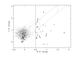
Figure 1: Colour-colour diagram of the IRAS 21324+5716 globule. Small dots are objects in and around the globule. Filled triangles are field stars with known spectral type (which mark the unreddened main sequence). Filled squares, arrows up (lower limit in J-H), and arrows right (lower limit in H-K and arbitrary J-H) mark reddened objects. The dashed line shows the criterion used to select these red sources. Dotted lines indicate the interstellar extinction path according to the extinction law of Mathis (1990eism.conf…63M (1990)). The two nearly vertical dotted lines mark extinctions of $A_{\rm V}$ = 10 and 20 mag. Note that the colour scales are in instrumental units.

3.2 Colour-colour diagrams and reddened sources

We show colour-colour diagrams for five of the nine globules, which contain more than 20 reddened objects, in Figs. 1-5. These figures contain a) datapoints for the IC 1396 objects as small dots, b) the main sequence datapoints as filled triangles, c) the extinction path calculated with the extinction law given by Mathis (1990eism.conf…63M (1990)) as dotted lines, d) reddened objects as filled squares and arrows. To allow a reliable comparison between the objects in IC 1396 and the standard stars, these diagrams are shown in instrumental magnitudes, which avoids colour mismatches. A rough transformation into the 2MASS photometric system can be obtained by adding about 0.3 mag to the H-K values. The diagrams show all datapoints in the 13′.5$\times$ 13′.5 field for each globule. We generally selected objects with H-K $>$ 0.5 mag as reddened sources. A more detailed discussion of the colour-colour diagrams and transformation of instrumental to 2MASS colours can be found in Appendix B.

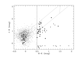
Figure 2: Colour-colour diagram of the IRAS 21346+5714 globule. Symbols as in Fig. 1.

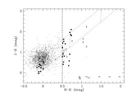
Figure 3: Colour-colour diagram of the IRAS 21352+5715 globule. Symbols as in Fig. 1.

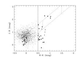
Figure 4: Colour-colour diagram of the IRAS 21445+5712 globule. Symbols as in Fig. 1.

Figure 5: Colour-colour diagram of the IRAS 22051+5848 globule. Symbols as in Fig. 1. For this globule the selection criterion for the reddened objects was shifted to H-K $>$ 0.7 mag, because all objects in this field show reddening of 0.2 mag.

As noted above, we found a large population of reddened objects for five of the nine globules. The remaining four globules contain only a small number of reddened sources. To assess the nature of all these red objects, we estimated the number of field stars in the direction of IC 1396 using the Besançon Galaxy model of Robin et al. (2003A&A…409..523R (2003)). This model is available online and is able to generate a photometry catalogue of objects in a certain Galactic direction with user-defined colour constraints. Our selection criterion for red objects was H-K $>$ 0.5 mag in instrumental colours, which translates into about H-K $>$ 0.8 mag in absolute colours.

In a first step, we executed several simulations with standard Galactic optical extinction (0.7 mag/kpc) and found that the number of objects with H-K $>$ 0.8 mag (and even with H-K $>$ 0.5 mag) is zero. This Galaxy model, however, does not include ultracool dwarfs with spectral types L and T. According to the DUSTY models of Chabrier et al. (2000ApJ…542..464C (2000)), evolved ultracool objects with T_eff = 1700 K have an H-K colour above 0.8 mag, and thus could be selected as red objects with our diagrams. On the other hand, objects with T_eff below 1300 K are too faint to be seen in our images. For this range of effective temperatures, Gizis et al. (2000AJ….120.1085G (2000)) give a space density of $2.11\cdot 10^{-3}\,pc^{-3}$. Our limiting magnitude constrains the distance at which we could detect these ultracool objects to $<$ 50 pc. With these values, the number of L-type objects in a 1 sqare degree field is $\approx$ 0.03. From this estimate, we conclude that the number of Galactic L-type stars in our red sample is negligible.

For this first calculation, however, we made the assumption of uniform Galactic extinction, which is not given in our fields, since we observe regions with high extinction in the direction of IC 1396. The Besançon Galaxy model is able to include clouds with a given distance and extinction. In a second set of simulations, we therefore assumed a cloud at a distance of IC 1396 (750 pc) with various extinction values ranging from A_V = 3 mag to A_V = 10 mag. The basic effect of such an additional cloud is that the main sequence in the colour-colour diagram is split. While the foreground objects remain unreddened, the background stars are shifted along the reddening path. From these simulations, we found that the background stars begin to exceed the H-K = 0.8 mag limit if the extinction of the cloud is higher than A_V = 5 mag. Thus, we expect a significant number of reddened background stars for globules with A_V $>$ 5 mag. According to the Galaxy model, these reddened objects will be mostly M type giants for a cloud with A_V = 5 mag, but with stronger extinction stars with earlier spectral types also would appear to have H-K $>$ 0.8 mag.

Based on these results, we can make the following conclusions about the nature of the reddened objects: We can exclude that our reddened objects contain a significant fraction of foreground stars. This includes also ultracool dwarfs with spectral types L and T. For globules with high extinction, we expect a significant number of highly reddened background stars, mostly late-type giants, along the reddening path. The remaining reddened sources, particularly the objects whose colours place them below the reddening path in the colour-colour diagram, should be young stellar objects (YSO) associated with the globules in IC 1396, which are intrinsically red because of excess emission from circumstellar matter. From photometry alone, it is not possible to unambiguously distinguish between YSOs and background stars.

Five of our nine globules clearly show a cumulation of reddened objects, whereas the number of reddened objects in the remaining four globules is $<$10. It is now interesting to analyse whether an excessive number of red objects is caused by a high density of YSOs in the globule or a high cloud extinction, leading to a high number of background stars which appear reddened. From the position of the reddened objects in the colour-colour diagram, we are able to get a rough idea of whether they are mostly YSOs or background stars, since background stars will be reddened along the reddening path, whereas YSOs may also appear below the extinction path. We define as YSO candidates all objects whose photometry does not rule out the possibility that they are located below the reddening band. This includes all objects with photometry in all three bands, which are below the reddening band, but also objects with upper limit in J, that could be located below the extinction band, and all reddened objects for which only K-band magnitudes are available. For each globule, we counted the number of YSO candidates and the total number of reddened objects. For globules without a large reddened population, it was found that only 77 % of the red sources are YSO candidates, whereas the remaining objects are in the extinction path. On the other hand, for globules with a large reddened population, the fraction of YSO candidates is 68%, i.e. significantly lower than in the ’empty’ globules. The most straightforward interpretation of this result is that the globules with many red objects have both a high density of YSO and strong extinction, leading to a high number of reddened background stars. The other globules possess smaller extinction values and fewer young stellar objects.

Assuming a distance of 750 pc for IC 1396 and no significant extinction, our reddened targets have absolute J-band magnitudes between 3.1 and 7.3 mag. This constrains the masses for these objects to a range roughly between 0.05 and 0.9 M_⊙ (Baraffe et al. 1998A&A…337..403B (1998)). Note that there are also no brighter sources significantly below the reddening path but with H-K $<$ 0.5 mag. Hence no unextincted Herbig AeBe stars are present. Since the globules show J-band extinction of at least 0.9 mag (see Table 1), there could be a few higher mass stars in our sample. On the other hand, it is unlikely that our faintest objects have substellar masses, rather than just being strongly influenced by extinction.

4 Extinction maps

4.1 Method

We determined extinction maps of the region 21${}^{\rm h}\!\!$.3 to 22${}^{\rm h}\!\!$.2 in R.A. and 56^∘ to 60^∘ in DEC (J2000) using accumulated star counts (Wolf-diagrams) in the 2MASS database. An example Wolf-diagram is shown in Fig. 12. Stars are counted in 3′ $\times$ 3′  boxes every 20″  down to the completness limit of the catalogue. A co-centred 1^∘ x 1^∘ sized field was chosen as ”unextincted” comparison. Minimum and maximum traceable extinction values are calculated and shown in Fig. 13, depending on the resolution used. We can trace about one to 20 mag optical extinction. Details of the star count method and the determination of the detection limits can be found in Appendix C.

4.2 Results

The extinction map of the whole IC 1396 field shows several regions of high extinction (see Fig. LABEL:obsfield). These are the globules around the star HD 206267, and a further group towards the north-east. We defined a ’globule’ as an object with an extinction of at least 3 $\sigma$ above the noise level and a size of at least 9 square arcminutes. With these criteria, an automated search using the SExtractor (Bertin & Arnouts 1996A&AS..117..393B (1996)) revealed 20 globules in IC 1396. Five of these globules were contained in the target list for our near-infrared survey with MAGIC from Schwartz et al. (1991ApJ…370..263S (1991)). The globules in this list that could not be detected in our extinction maps possess sizes and masses below our detection limits (see also Patel et al. 1995ApJ…447..721P (1995)). Adding the remaining five objects from this list, there are 25 dark clouds in the field. The large region of high extinction at about (21${}^{\rm h}\!\!$.73:58.8$\degr$) is caused by the bright star $\mu$ Cep, which prevented the detection of stars in its vicinity. Similarly the star $\zeta$ Cep at (22${}^{\rm h}\!\!$.19:58.2$\degr$) causes such a fake globule. The full list of all globules with their coordinates and known identifications is given in Table 1. Figure 6 shows as examples the extinction maps for the globules where we detected a large number of reddened sources.

Figure 6: Contour plots of the extinction obtained from the J-band 2MASS data for the globules 11 (upper left), 3 (upper right), 9 (lower left), and 4 and 5 (lower right). Contours start at 1 mag optical extinction and increase by 1 mag. Conversion from extinction in the J-band to optical extinction was done according to Mathis et al. (1990eism.conf…63M (1990)). Dashed lines mark the borders of the observed NIR fields. $+$ signs indicate reddened objects in the reddening path, while circles mark the YSO candidates, and arrows the principle direction towards the O6.5V star HD 206267. Note that the contours are slightly smoothed and hence peak extinction values are somewhat lower than in Table 1.

To measure the mass we integrated the total extinction in the globules (A${}_{\rm V}^{\rm tot}$). Only regions with an extinction above the one sigma noise level where considered, and the outer radius of the globule was taken as the size given by the SExtractor software (FWHM, assuming a Gaussian core). From these integrated extinction values we determined the mass of the globules using the fact that the column density N(H) of hydrogen atoms can be expressed as 6.83 10²¹ cm^-2 $\times$ A_V/R_V where R_V is typically 3.0 (see e.g. Mathis 1990eism.conf…63M (1990)). Using a distance of 750 pc for the globules, and the 20″  pixel scale in our maps, the total mass in a globule can be determined from the integrated optical extinction (A${}_{\rm V}^{\rm tot}$) in the globule by: M_glob $[$M${}_{\odot}]$ = 0.098 A${}_{\rm V}^{\rm tot}$ $[{\rm mag}]$. Note that the obtained extinction values are averaged over the box-size of 3′ $\times$ 3′. If the dust is concentrated in a smaller area, the obtained masses are lower limits. The error of the estimated mass depends on the mean extinction within the globule compared to the noise level in our map. As a typical value we find that the mean extinction is about 5 $\sigma$ of the noise level and hence the uncertainties in the inferred masses are about 20 %. In the case of IC 1396 N we can compare our mass estimate with literature values. Wilking et al. (1993AJ….106..250W (1993)) estimate 380 M_⊙ and Serabyn et al. (1993ApJ…404..247S (1993)) give 480$\pm$120 M_⊙ within the central 0.3 pc. Given the large uncertainties and the fact that the object is rather small and the mass is concentrated close to the actual star forming core (see e.g. Codella et al. 2001A&A…376..271C (2001)), our lower limit for the whole globule of 300 M_⊙ agrees well with these estimates. Weikard et al. (1996A&A…309..581W (1996)) give an estimate of 12000 M_⊙ for the total mass of their mapped region (about six square degrees centred on HD 206267). The mass estimated from our extinction maps in the same field is 9000 M_⊙, reasonably close.

Within the errors of about 20 % the total optical extinction values and globule masses, obtained from the J- and H-band 2MASS data, are consistent. Some of the masses calculated with the K-band data differ by a larger amount. There are two groups of objects: 1) The mass from the K-band data is much smaller than the mass obtained from the J- and H-band data. The reason could be that the globule contains an embedded cluster of stars. These stars are easier to detect in K and hence decrease the apparent extinction. In these cases the given masses M_J,H are lower limits for the globule mass. 2) The mass from the K-band data is much larger than the mass obtained from the J- and H-band data. An explanation could be that the conversion of extinction in the K-band to optical extinction cannot be performed following Mathis et al. (1990eism.conf…63M (1990)) that assume an opacity index of 1.7. A lower value might be valid in these globules. Note that this effect could counter-balance 1) in the case of an embedded cluster.

5 Globule properties

Table 1: All detected globules in the IC 1396 region. The upper part of the table lists the objects observed with MAGIC in JHK, while in the lower part the additional globules detected in our extinction maps are given. Column 4 lists the projected distance of the globule from the exciting star HD 206267. The size in square arcminutes is the value we obtained from the SExtractor software (a ? marks the globules that were not detected in the extinction maps.). Column 6 contains the number of reddened objects (in brackets: number of YSO candidates as defined in Sect. 3.2). In columns 7 to 9 we give the peak extinction values in the three filters obtained from our extinction maps, while columns 10 to 12 list the masses estimated for the globules. ^∗ The given masses are measured for both globules together.

Nr.	Name(s)	($\alpha$;$\delta$) (J2000)		Distance	Size	Red stars	AJ	AH	AK	MJ	MH	MK
		[h m]	[° ′ ]	[pc]	[$\Box\arcmin$]		[mag]			[M⊙]
1	IRAS 21246+5743	21 26	57 58	24.7	114	31(18)	3.1	1.9	1.3	515	541	401
	IC 1396 W
2	IRAS 21312+5736	21 33	57 50	11.7	?	9(7)	0.9	0.7	0.7
3	IRAS 21324+5716	21 34	57 32	8.6	50	27(20)	2.0	1.2	1.1	224	182	207
	LDN 1093
	LDN 1098
4	IRAS 21346+5714∗	21 36	57 28	5.4	?	51(38)	1.1	1.0	0.7	120	119	74
5	IRAS 21352+5715∗	21 37	57 30	3.1	?	36(22)	0.8	0.7	0.6	120	119	74
	LDN 1099
	LDN 1105
6	IRAS 21354+5823	21 37	58 37	15.2	?	4(3)	0.9	0.8	1.1
	LDN 1116
7	IRAS 21388+5622	21 40	56 36	12.3	?	7(5)	0.9	0.7	0.9
8	IRAS 21428+5802	21 44	58 17	13.8	?	10(8)	1.1	0.9	0.9
	LDN 1130
9	IRAS 21445+5712	21 46	57 26	13.2	?	24(16)	0.9	0.8	0.7	120	141	195
	IC 1396 E
10	IRAS 21539+5821	21 55	58 35	32.9	115	–	2.0	1.3	0.9	374	351	458
11	IRAS 22051+5848	22 07	59 08	55.9	226	51(36)	2.7	2.1	1.5	788	714	847
	LDN 1165
	LDN 1164
12		21 25	57 53	25.5	77		1.8	1.4	1.5	279	285	187
13		21 25	58 37	29.3	50		1.4	0.9	1.1	160	158	109
14	LDN 1086	21 28	57 31	19.4	50		1.5	1.1	1.0	273	273	233
15		21 33	59 30	29.2	39		1.1	1.1	1.1	86	146	160
16	LDN 1102	21 33	58 09	14.0	46		1.4	1.1	1.2	189	182	206
17	LDN 1088	21 38	56 07	18.6	64		1.4	1.0	0.8	298	299	372
18	LDN 1131	21 40	59 34	28.2	45		1.6	1.2	1.1	265	303	305
19	IC 1396 N	21 40	58 20	11.6	84		1.5	1.2	1.0	285	294	271
20	LDN 1131	21 41	59 36	28.6	87		1.6	1.2	1.2	390	353	452
21	LDN 1129	21 47	57 46	14.9	147		1.4	1.0	0.9	385	403	498
22		21 49	56 43	21.3	70		1.2	0.9	0.8	207	199	311
23	LDN 1153	22 01	58 54	44.7	270		2.3	1.7	1.2	927	875	933
24	LBN 102.84+02.07	22 08	58 23	53.7	74		1.7	1.3	0.9	402	382	376
25	LBN 102.84+02.07	22 08	58 31	54.1	36		1.3	1.1	0.9	201	205	247

With the results of Sect. 3 and 4, a homogeneous sample of globules is now at our disposal (see Table 1). To evaluate possible trends in this dataset, we selected the following globule properties and tested them for correlations: projected distance of the globule from the exciting O star HD 206267, projected size of the globule, number of YSO candidates within the field of the globule, peak extinction value, total mass, mean column density within the globule (total mass divided by the size). For each pair of these properties, we fitted their relationship linearly and calculated the correlation coefficient $r$. Since the value $t=r\sqrt{\frac{(N-2)}{1-r^{2}}}$ ($N$: number of datapoints) follows Student’s $t$-distribution, this gives us the probability that the two parameters show indeed a significant correlation. In order to perform these tests, we set globule sizes to 30 square arcminutes and masses to 120 M_⊙, if they could not be determined. These values are the upper limits from our detection procedure for globules in the extinction maps. As peak extinction, we used the values from the J-band, since they have the best signal-to-noise ratio.

The best correlations are obtained when comparing size and mass, peak extinction and mass, and size and peak extinction. The false alarm probabilities (FAP) for linear relationships between these three parameters are below $10^{-3}$ %. These are expected correlations, since the mass is proportional to the mean extinction and the size of the globule. The correlation of size and peak extinction might be due to our method that smooths the extinction over a 3′ $\times$ 3′  field, naturally leading to lower peak extinction values for small globules.

Additionally, we found a non-obvious correlation between mass $M$ and distance $d$ from the exciting star: Globules farther away from HD 206267 have on average larger masses. The least-square fit gives $M[M_{\odot}]=8.6\,d\,[pc]+84$, and the FAP for this correlation is 0.078 %. We repeated this test excluding the four globules with $d>40$ pc, because it might be that these regions are too far away from HD 206267 to be influenced by its radiation. Without the data points for these globules, the FAP is still only 2.2 %. Thus, there is a significant connection between globule mass and distance from the exciting star (see Fig. 7).

There are two possible explanations for this correlation: 1) The mass loss rate of a cloud induced by photo-ionisation of the external layers is inversely proportional to the distance from the exciting star (see e.g Codella et al. 2001A&A…376..271C (2001)). Hence, more distant globules do not lose as much mass due to evaporation. 2) Globules closer to the exciting star contain more young objects (see below) and hence the mass estimates of these globules lead to too low values due to the star count method. Connected to the distance-mass correlation are correlations of distance and globule size as well as distance and peak extinction value. These are consequences of the interrelations described in the above paragraph.

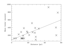
Figure 7: Globule masses vs. distance from the exciting O star. A linear least-square fit is shown as dashed line. This correlation has a FAP of 0.078 %. If we exclude the four globules with $d$ $>$ 40 pc, the correlation is still significant with a FAP of 2.2 %.

The remaining combinations of parameters show no significant correlations, i.e. with FAP below 10 %. Particularly, we see no correlation between distance and number of YSO candidates. This can be used to rule out the second explanation for the mass-distance correlation. This relationship is therefore most likely related to mass loss via photo-evaporation, as explained above. For all correlation tests that use the number of YSO candidates, we are restricted to those globules in which red objects were identified (see Table 1). Thus, small number statistics hamper the correlation tests for these parameters.

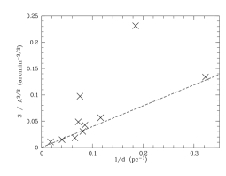
Figure 8: Diagram of star density vs. inverse distance from the exciting O star. A linear least square fit is shown as dashed line. The correlation has a FAP of 2.5 %. If we exclude globules with $d$ $>$ 40 pc a FAP of 5.0 % is still reached.

How do these findings fit in a scenario where the radiation pressure of the O star is the primary triggering mechanism for star formation in the globules? In a first order interpretation, we assume that the density of young objects $S/A^{3/2}$ (S - numer of YSO candidates; A - projected size of the globule) is positively correlated with the mass of the globule $M$ and the pressure $P$ exerted by the radiation flux $\Phi$ from the star: $S/A^{3/2}\propto M\times P$. The radiation pressure or ionising flux is inversely proportional to the square of the distance ($P\propto\Phi\propto d^{-2}$; Codella et al. 2001A&A…376..271C (2001)) and the mass is proportional to the distance ($M\propto d$ as shown in Fig. 7). Hence we should expect a correlation of the star density with the inverse distance from the star: $S/A^{3/2}\propto M\times P\propto d^{-1}$. Indeed, such a correlation is seen tentatively in our data. A linear fit gives $S/A^{3/2}=0.555d^{-1}$, with a FAP of 2.5 % (see Fig. 8). If we exclude the one globule with $d>40$ pc, the FAP increases to 5.0%. Although this result clearly needs to be substantiated with more datapoints, it tentatively confirms our initial assumption that the star forming activity is driven by the radiation pressure of the O star.

We re-examined the conclusion of Sect. 3.2 where we found that globules with a rich population of young stars also show high extinction leading to a high number of reddened background objects. Although there is no correlation between extinction A_J and the number of YSO candidates $N$, the data show a clear tendency: All globules with $N$ $<$ 10 have A_J $\leq$ 1.1 mag. On the other hand, 50 % of the globules with $N$ $>$ 10 exhibit A_J $\geq$ 2 mag. Thus, globules that harbour many red objects tend to show high extinction values, confirming our result from Sect. 3.2.

We further investigated the positions of the YSO candidates in the globules with respect to the direction of the O6.5V star HD 206267. Figure 6 shows the positions of the reddened sources overplotted on the extinction map for the five globules where a large number of reddened objects was found (the two overlapping fields are combined in one figure). In three of the fields the YSO candidates (circles) seem to be preferentially positioned towards the direction of the exciting O6.5V star. Objects within the reddening path (plus signs) seem to be more concentrated towards the high extinction regions. This picture agrees well with the expectations of triggered star formation via radiation-driven implosion, although this behaviour is not present in all investigated globules.

6 New HH objects and H₂ outflows

Table 2: Coordinates of the brightest knots in the newly detected Herbig-Haro objects. ^∗ Counterparts of the optical knots detected in H₂ in Froebrich & Scholz (2003A&A…407..207F (2003)).

Object	H${}_{2}^{*}$	$\alpha$(J2000)	$\delta$(J2000)
		[h m s]	[°  ′  ″ ]
HH 588 NE3		21 41 00.0	56 37 19
		21 41 01.0	56 37 25
HH 865 A		21 44 28.5	57 32 01
		21 44 29.3	57 32 24
HH 865 B		21 45 10.5	57 29 51
HH 864 A	2-j	21 26 01.4	57 56 09
	2-j	21 26 02.0	57 56 09
HH 864 B	5	21 26 07.9	57 56 03
HH 864 C	2-b	21 26 21.3	57 57 40
	2-d	21 26 18.6	57 57 12

In our observed field there are several known Herbig-Haro objects and outflows. These are mainly the well investigated flows in the IC 1396 N globule (HH 589-595 found by Ogura et al. 2002AJ….123.2597O (2002) and HH 777-780 discovered by Reipurth et al. 2003ApJ…593L..47R (2003)). The H₂ outflow from IC 1396 W which was shown in Froebrich & Scholz (2003A&A…407..207F (2003)) has no published optical emission counterpart. Connected to IRAS 21388+5622 is the HH 588 object (Ogura et al. 2002AJ….123.2597O (2002)). In the IRAS 22051+5848 field a giant outflow HH 354 was found by Reipurth & Bally (2001ARA&A..39..403R (2001)).

In our [SII] images we were able to re-discover all of the known HH objects around IC 1396 N. The whole field is full of extended emission line objects (visible as excess emission in the [SII] images compared to the I-band fluxes). These filaments are excited by the strong UV emission of the O6.5V star HD 206267. Many of these filaments show a similar appearance to some of the HH objects near IC 1396 N. Hence, it is very difficult to decide from the shape of the emission alone if we see an outflow or just UV excited filaments. This might be the reason why HH 777 was not mentioned by Ogura et al. (2002AJ….123.2597O (2002)) although it is clearly visible in their image.

We also detect the HH 354 and HH 588 flows from IRAS 22051+5848 and IRAS 21388+5622, respectively. There is an additional emission feature 1$\arcmin\!\!$.4 east of HH 588 NE2, consisting of two fuzzy blobs (for positions see Table 2). This object was slightly outside the field shown in Ogura et al. (2002AJ….123.2597O (2002)). The knot-like appearance of this object suggests an HH object (HH 588 NE3) connected to the HH 588 flow, rather than being a UV-excited emission feature (see Fig. 9). None of the optical emission features of HH 588 is detected in our H₂ images.

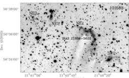
Figure 9: [SII] image of the HH 588 region. The newly detected emission knots HH 588 NE3 are seen in the upper left corner.

We detected two new groups of HH objects in our optical field. We found the H₂ flow from IC 1396 W also in [SII] and call it HH 864 (see Fig. 10). The bright H₂ knot 2-j (Froebrich & Scholz 2003A&A…407..207F (2003)) has a [SII] counterpart (HH 864 A) which shows a bow shape with two maxima in the emission. The two knots (2-b and 2-d) in the north-eastern lobe are visible in the optical emission line also (HH 864 C). Knot 5 (50″  east of 2-l) has an optical counterpart as well (HH 864 B). It is still not clear if this emission knot is connected to the IRAS 21246+5743 source or another (unknown) source in the IC 1396 W globule.

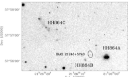
Figure 10: Our [SII] image of the outflow from IC 1396 W (HH 864) shows clearly some of the brightest emission knots, previously detected in H₂ by Froebrich & Scholz (2003A&A…407..207F (2003)).

We find in our optical field a giant flow emerging from the IRAS 21445+5712 source, which is also called IC 1396 E. There are two bright bow shocks heading to the north-west of the source, HH 865 A and HH 865 B (see Fig. 11). The distance of about 0.2°  of the terminating bow HH 865 A from the source makes this flow 2.6 pc in length in one lobe (assuming a distance of 725 pc). No counterflow is found in our images. The globule was also observed in H₂. The closer of the two bow shocks is unfortunately just outside our NIR field and hence could not be detected. There is no H₂ emission in our image that might be connected to this flow. Only a few very faint features are found south and east of the IRAS source. These are UV excited emission coinciding with cloud borders.

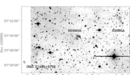
Figure 11: The new flow HH 865 in the [SII] filter, heading away from the possible driving source IRAS 21445+5712.

In IRAS 21312+5736 we see some faint H₂ filaments that might be UV excited. The field of IRAS 21324+5716 is full of bright H₂ emission features coinciding with the optical emission. This applies also for the neighbouring fields IRAS 21346+5714 and IRAS 21352+5715. No H₂ features are detected near IRAS 21354+5823, IRAS 21428+5802, IRAS 21539+5821 and IRAS 22051+5848.

7 Summary and discussion

NIR observations of IC 1396 in conjunction with extinction maps obtained from 2MASS data reveal star forming activity and a large number of globules in this region. Twenty five globules were identified using our extinction maps and the list of Schwartz et al. (1991ApJ…370..263S (1991)). Four of them were previously uncatalogued in the SIMBAD database. In all but four cases the masses (or at least lower limits) of the globules could be determined. Also the size could be measured properly for all but seven objects.

For nine globules observed deeper than 2MASS in this work, the content of heavily reddened objects was derived by means of colour-colour diagrams. Five of these globules exhibit a rich population of red objects. At least half of these objects are good candidates for young stellar objects, the remaining half is probably contaminated by reddened background stars. The five globules with many red objects include the targets with the highest extinction values, suggesting a correlation of the strength of the star formation activity with the mass of the globule.

Star formation in small globules is often thought to be strongly influenced by the radiation pressure of a nearby bright star. It was therefore investigated how the globule properties in IC1396 depend on the distance from the O star HD 206267. The masses of the globules show a clear positive correlation with the distance from this star. We conclude that evaporation due to photo-ionisation affects the mass distribution of the globules around HD 206267. Our data are consistent with a scenario in which the radiation pressure from the O star regulates the star forming activity (expressed as density of young sources) in the globules, in the sense that the radiation pressure compresses the gas and thus leads to enhanced star formation.

Our optical data lead to the discovery of several new HH objects. These are the counterpart of the previously known H₂ emission of the flow from IC 1396 W and a new parsec scale flow from IC 1396 E. Further a new emission knot belonging to the known HH 588 object was discovered.

Appendix A Reliability of instrumental photometry

Several tests were executed to evaluate the reliability of the instrumental photometry. Since we observed each globule at least twice (and six of them three times), we can compare the instrumental magnitudes from different mosaics of the same region to look for systematic mismatches. With one exception (see below), we found good agreement within $\pm 0.05$ mag. The photometry from mosaics which were taken under non-photometric conditions (see Sect. 2.1) shows the highest deviations, as expected. These deviations, however, affect all broadband mosaics equally, thus they are not visible in the colours. For one field (IRAS 21539+5821) we see large systematic photometry mismatches between all mosaics, which are also visible in the colours. The most probable explanation is variable weather conditions, e.g. cirrus clouds which we did not recognise during the observations. We excluded this field from all further analysis.

As mentioned in Sect. 2.1, all broad-band images were obtained at low airmass; the maximum airmass difference is 0.45. Since the NIR extinction coefficient on Calar Alto is usually below 0.1 mag/airmass (Hopp & Fernández hf02 (2002)), the differential extinction offsets between the instrumental magnitudes of different fields are safely below 0.05 mag. More important, the extinction coefficient in the NIR is nearly wavelength independent. Therefore, differential extinction does not significantly affect the colours of our targets. Thus, we did not perform an extinction correction. Another test of our photometry was enabled by field overlap of the mosaics around IRAS 21346+5714 and IRAS 21352+5715. Again we found no significant offsets between the colours of the targets which were detected in both fields. For these reasons, we conclude that the instrumental colours of the targets observed under photometric conditions are reliable.

If available, the deep, stacked mosaics of the globules were calibrated by measuring the magnitude offsets to a mosaic obtained under photometric conditions and applying these offsets to the instrumental magnitudes of the deep mosaics. Thus, the photometry of the deep mosaics is now directly comparable with all other data obtained under photometric conditions, in particular with the standard star main sequence.

Appendix B Colour-colour diagrams and absolute calibration

For the colour-colour diagrams, we used the photometry from the deep mosaics if more than one mosaic is available, otherwise the photometry from the single mosaic. We only consider objects with errors below 0.2 mag. There are, however, only very few objects (typically below 1%) with larger errors.

The bulk of the IC 1396 objects in the diagrams coincides with the late-type end of the main sequence. There is one exception – Fig. 5 – which will be discussed below. This is expected because most stars are late-type. Moreover, giant stars also concentrate towards the late-type end of the main sequence. Since our main sequence ends at spectral type K8, it is not surprising that there are many field objects above the upper end of this sequence. These could be M-type dwarf or giant stars. The bulk of the field objects is (again with one exception) always in the same position in each diagram, which makes us confident that the colours from the different fields can be compared with each other.

There is one field (IRAS 22051+5848, see Fig. 5), where the bulk of the datapoints is clearly offset by about 0.2 mag in (H-K) and 0.2 mag in (J-H), i.e. roughly in the direction of the reddening vector. This field shows large-scale structures of nebulosity and large voids without any objects, indicative of strong extinction. Thus, in this field background objects are probably significantly reddened because their light must pass through extended regions of dust. The 0.2 mag offset in both colours then corresponds to a mean visual extinction of A${}_{\rm V}\approx 2$ mag.

We are now interested in detecting objects whose position in the colour-colour diagram indicates significant intrinsic reddening, i.e whose position is clearly shifted in the direction of the extinction path or even below these lines. The following criteria were used to select such reddened objects:

a) If an object is detected in all three filters, its H-K colour should exceed 0.5 mag: H-K $>$ 0.5 mag. (For the IRAS 22051+5848 field, we require H-K $>$ 0.7 mag, because all objects in this field show a 0.2 mag shift in H-K, see above.) Objects that satisfy this condition are shown as filled squares in the diagrams.

b) If the object is only detected in H and K, we demand again that H-K $>$ 0.5 mag (or $>$ 0.7 mag for IRAS 22051+5848). These objects are marked with an ’arrow up’, and their J-H colour is a lower limit estimated from the H-band photometry and our sensitivity limit in the J-band.

c) If the object is only detected in K, we can only determine a lower limit for the H-K colour by subtracting the K-band photometry from the sensitivity limit in the H-band. We require that this lower limit is $>$ 0.5 mag (or $>$ 0.7 mag for IRAS 22051+5848). These objects are shown with an ’arrow to the right’, and their J-H colours are chosen arbitrarily.

We selected all objects that satisfy one of these conditions and examined these targets in the images. We rejected all objects that are clearly not star-shaped (i.e. galaxies or H₂ emission knots), as well as spurious detections (i.e. cosmics or spikes of bright stars). The remaining objects are good candidates for objects with intrinsic reddening in the globules. This selection might be incomplete, since some young objects could have H-K $<$ 0.5, and thus would fall out of our selection criteria. As noted above, the colour-colour diagrams contain only objects with errors below 0.2 mag. With larger error bars a reliable separation between reddened and unreddened objects is not possible. In most cases, however, the objects with errors $>$ 0.2 mag do not appear strongly reddened.

After this selection process, the globules clearly fall in two groups: Four of them show only very few reddened objects, i.e. their number is $\leq$ 10. The remaining five globules harbour more than 20 reddened objects, in two cases (IRAS 21346+5714, IRAS 22051+5848) the number of reddened objects is larger than 50. For these five globules we show the colour-colour diagrams in Figs. 1-5.

As noted above, the colours in the diagrams are instrumental. We determined, however, the offsets to the photometric system of the 2MASS catalogue, which is available online. For all detected objects, we searched for counterparts in the 2MASS database. In each field, several hundred common objects were identified. For these objects, we determined the average offset $\Delta$ between 2MASS photometry and our instrumental magnitudes in J, H, and K. These offsets (called $\Delta_{J}$, $\Delta_{H}$, $\Delta_{K}$ in the following) include a zero-point as well as extinction correction.

The offsets in a certain band are not constant for all globules; they differ by as much as 0.3 mag, depending on the weather conditions during the observations (see above). The difference between the offsets, in particular the values of $\Delta_{J}-\Delta_{H}$ and $\Delta_{H}-\Delta_{K}$, are comparable for all globules, confirming again that the relative colours are reliable. We obtain $\Delta_{J}-\Delta_{H}=0.03\pm 0.06$ and $\Delta_{H}-\Delta_{K}=0.29\pm 0.08$. Thus, our colour-colour diagrams can be roughly transformed into the 2MASS photometric system by adding 0.3 mag to the H-K values. We note, however, that this transformation does not include colour terms, which means that the offsets are probably not constant for all colours, in particular not for the main sequence and the reddened targets (see Froebrich & Scholz 2003A&A…407..207F (2003)). This was the main reason why we kept the diagrams in the instrumental colours, as described above.

The absolute calibration also allows us to estimate the sensitivity limit of our survey, i.e. the faintest objects for which a 5$\sigma$ detection is possible. We reach about 17.0 mag in J, 16.5 mag in H, and 16.0 mag in K. For comparison, the 2MASS catalogue for this region contains objects down to 16.9 mag in J, 16.1 mag in H, and 15.6 mag in K. Our images are thus significantly deeper than the 2MASS catalogue for this region, particularly in the H- and K-band.

Appendix C Extinction map determination

A determination of absolute magnitudes of the stars within the globules, as well as an estimation of the dust mass in the globules, requires a measurement of the extinction. As discussed above, the assumption of a uniform Galactic extinction is not valid in our field. There are local extinction enhancements connected to the globules and even within these small clouds the dust and so the extinction is not uniformly distributed. Hence we need to determine the local extinction enhancements for our globules, compared to the neighbouring star field. These extinction enhancements will be used to estimate the mass of the globules by adopting a distance of 750 pc. Measuring the extinction from colour-colour diagrams is relatively difficult due to the photometric errors and the large scatter of the main sequence (see e.g. our Figs. 1-5). Hence this method only allows a rough estimate of at best $\pm$ 3 mag of the optical extinction averaged over the whole globule and is in particular not able to determine the extinction/mass distribution within the globules. A more accurate method is to create accumulative star counts (Wolf diagrams) as described e.g. in Kiss et al. (2000A&A…363..755K (2000)). Since we expect high extinction values within the globules (A_V $\geq$ 5 mag), creating these diagrams from NIR observations obviously is the best choise. The 2MASS database provides an ideal basis for this purpose.

units ¡10.5mm,17mm¿ point at 0 0 x from 10 to 17 , y from -0.5 to 2.2 10.0 -0.39794 10.1 -0.30103 10.2 -0.30103 10.3 -0.30103 10.4 -0.22184 10.5 -0.22184 10.6 -0.15490 10.7 -0.15490 10.8 -0.09691 10.9 -0.04575 11.0 0.00000 11.1 0.04139 11.2 0.07918 11.3 0.11394 11.4 0.14612 11.5 0.20412 11.6 0.23044 11.7 0.27875 11.8 0.30103 11.9 0.34242 12.0 0.38021 12.1 0.41497 12.2 0.46239 12.3 0.50515 12.4 0.54406 12.5 0.57978 12.6 0.61278 12.7 0.65321 12.8 0.69019 12.9 0.72427 13.0 0.75587 13.1 0.79934 13.2 0.83250 13.3 0.86332 13.4 0.89762 13.5 0.93449 13.6 0.97312 13.7 1.00860 13.8 1.04139 13.9 1.07918 14.0 1.11059 14.1 1.14613 14.2 1.18184 14.3 1.21484 14.4 1.24797 14.5 1.28103 14.6 1.31387 14.7 1.34635 14.8 1.37840 14.9 1.40993 15.0 1.44248 15.1 1.47422 15.2 1.50651 15.3 1.53782 15.4 1.56820 15.5 1.59879 15.6 1.62839 15.7 1.65801 15.8 1.68842 15.9 1.71850 16.0 1.74819 16.1 1.77597 16.2 1.80754 16.3 1.84011 16.4 1.86982 16.5 1.90037 16.6 1.92840 16.7 1.95376 16.8 1.96661 16.9 1.97313 17.0 1.97313 / 10.0 -0.04575 10.1 -0.04575 10.2 0.00000 10.3 0.04139 10.4 0.07918 10.5 0.11394 10.6 0.14612 10.7 0.17609 10.8 0.20412 10.9 0.23044 11.0 0.27875 11.1 0.32221 11.2 0.36172 11.3 0.41497 11.4 0.44715 11.5 0.47712 11.6 0.51851 11.7 0.55630 11.8 0.59106 11.9 0.62324 12.0 0.66275 12.1 0.69897 12.2 0.73239 12.3 0.76342 12.4 0.79934 12.5 0.83250 12.6 0.86923 12.7 0.90309 12.8 0.93951 12.9 0.96848 13.0 1.00432 13.1 1.04139 13.2 1.07555 13.3 1.11059 13.4 1.14301 13.5 1.17898 13.6 1.21219 13.7 1.24551 13.8 1.27875 13.9 1.31175 14.0 1.34242 14.1 1.37291 14.2 1.40483 14.3 1.43297 14.4 1.46240 14.5 1.49415 14.6 1.52375 14.7 1.55509 14.8 1.58433 14.9 1.61490 15.0 1.64640 15.1 1.67761 15.2 1.70927 15.3 1.74036 15.4 1.77232 15.5 1.80209 15.6 1.83569 15.7 1.86629 15.8 1.89542 15.9 1.91960 16.0 1.93702 16.1 1.94645 16.2 1.94939 16.3 1.95036 16.4 1.95085 16.5 1.95085 16.6 1.95085 16.7 1.95085 16.8 1.95085 16.9 1.95085 17.0 1.95085 / 10.0 0.04139 10.1 0.07918 10.2 0.11394 10.3 0.14612 10.4 0.17609 10.5 0.20412 10.6 0.23044 10.7 0.27875 10.8 0.32221 10.9 0.36172 11.0 0.39794 11.1 0.43136 11.2 0.47712 11.3 0.50515 11.4 0.54406 11.5 0.57978 11.6 0.62324 11.7 0.65321 11.8 0.68124 11.9 0.71600 12.0 0.75587 12.1 0.79239 12.2 0.81954 12.3 0.85125 12.4 0.88649 12.5 0.92427 12.6 0.95904 12.7 0.99563 12.8 1.02938 12.9 1.06446 13.0 1.09691 13.1 1.13033 13.2 1.16732 13.3 1.19866 13.4 1.23553 13.5 1.26717 13.6 1.29885 13.7 1.33041 13.8 1.35984 13.9 1.39094 14.0 1.41996 14.1 1.44716 14.2 1.47712 14.3 1.50651 14.4 1.53908 14.5 1.56937 14.6 1.59988 14.7 1.63347 14.8 1.66370 14.9 1.69373 15.0 1.72673 15.1 1.75891 15.2 1.79169 15.3 1.82413 15.4 1.85309 15.5 1.87506 15.6 1.88705 15.7 1.89098 15.8 1.89098 15.9 1.89098 16.0 1.89098 16.1 1.89098 16.2 1.89098 16.3 1.89098 16.4 1.89098 16.5 1.89098 16.6 1.89098 16.7 1.89098 16.8 1.89098 16.9 1.89098 17.0 1.89098 /

16.6 2.2 16.6 -0.5 / 15.6 2.2 15.6 -0.5 / 15.2 2.2 15.2 -0.5 /

left label logN ticks in long numbered from -0.5 to 2.0 by 0.5 short unlabeled from -0.5 to 2.2 by 0.1 / right label ticks in long unlabeled from -0.5 to 2.0 by 0.5 short unlabeled from -0.5 to 2.2 by 0.1 / bottom label apparent brightness [mag] ticks in long numbered from 10 to 17 by 2 short unlabeled from 10 to 17 by 0.5 / top label ticks in long unlabeled from 10 to 17 by 2 short unlabeled from 10 to 17 by 0.5 /

Figure 12: Example of a Wolf diagram for the three filters (J - solid; H - dashed; K - dotted) at $\alpha$ = 21^h52^m00^s $\delta$ = 57°00′00″  (J2000). The accumulated number of stars N is averaged over a 1° x 1°field and normalised to an area of nine square arcminutes. The vertical lines correspond to the completeness limit in JHK (line type as for the Wolf diagrams) at which we measured the extinction. The mean slope $<$X$>$ varies with the filter (0.36 for J and 0.34 for H and K) and also with the position on the sky. As can be seen the slope is also not constant, due to extinction from the ISM (the slope in J ranges from 0.38 (at 11 to 12 mag) to 0.30 (at 15 to 16 mag)).

Using star counts to estimate the extinction is based on several assumptions: 1) The stars are equally distributed and all apparent voids or less densely populated regions are caused by extinction. 2) All stars possess the same absolute brightness. 3) The completeness limit of the input catalogue does not depend on the position in the sky. Since in general these assumptions are not valid, we performed our star counts in a way that ensures as small as possible errors due to the assumptions made. 1) As reference or control field we choose a 1^∘ x 1^∘ field around the position where the stars are counted. This running average ensures that large scale variations in the average star numbers due to Galactic position or large scale structures are corrected. 2) The box size in which we count the stars for each position was varied between 1′$\times$1′  and 5′$\times$5′. In boxes larger than 3′$\times$3′  of the order of 100 stars are enclosed on average. This ensures that we enclose a ’typical’ sample of stars in our box, that represents the ’average’ star very well. 3) The completeness limit of the 2MASS catalogue varies over the field. Star counts where hence only performed down to a magnitude to which the catalogue is complete over the whole field (J=16.6, H=15.6, K=15.2).

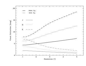
Figure 13: Minimum and maximum values of optical extinction that could be traced with our extinction maps obtained from the 2MASS data in JHK, using different box sizes. A_V values are determined from extinction in JHK using the conversion factors given in Mathis et al. (1990eism.conf…63M (1990)).

In order to investigate not only the extinction distribution in our globules but also the large scale dust distribution in the entire Cep OB 2 region, we created an extiction map of the whole field, ranging from 21${}^{\rm h}\!\!$.3 to 22${}^{\rm h}\!\!$.2 in R.A. and from 56^∘ to 60^∘ in DEC (J2000). In Fig. LABEL:obsfield we show an example of the extinction map obtained from the J-band 2MASS data. Since we had a large amount of data to process we decided to parallelise the problem. We wrote an MPI-parallel C++ code in order to get maximum performance from our 32-node hyperthreaded cluster of the so-called ”Beowulf” type. It took 13 hours to process all the data on this cluster - without the parallelisation of the problem it would have taken of the order of 60 times as long (about 33 days).

For the star counts we selected all 2MASS objects in our field with a signal-to-noise ratio of larger than five (quality flag A, B, or C). With this selection criteria we extracted 841908, 783474, and 635478 objects in JHK, respectively. This converts to an average density of stars of about 1 star per 20″ x 20″  field. Hence, we performed the star counts every 20″  in order to obtain the final extinction map. This method ensures a maximum gain of information from the 2MASS catalogue. Figure 12 shows an example of a Wolf diagram in each of the three filters at $\alpha$ = 21^h52^m00^s $\delta$ = 57°00′00″  (J2000). In order to find the best compromise between box-size and extinction regime that can be traced, the box-sizes were varied in steps of 0′.25. Depending on the box-size the average number of stars in the boxes varies and hence we can trace different extinction regimes. In Fig. 13 we plot the minimum and maximum value of traceable extinction (converted to A_V) with our method in IC 1396, depending on the chosen box-size and the three 2MASS filters. The lower limit (A${}_{\lambda}^{\rm min}$) is calculated from the three sigma noise level of the determined extinction in the whole Cep OB 2 field. This limit can be transformed into a ratio F_σ/F_back by

$${\rm A}_{\lambda}^{\rm min}=-\frac{1}{\rm X}*\log{\left(1-\frac{{\rm F}_{\sigma}}{{\rm F}_{\rm back}}\right)}.$$ (1)

F_σ is the noise of the number of stars in the star count map. If this number of stars is missing in the presence of F_back stars in the comparison field, an apparent extinction of A${}_{\lambda}^{\rm min}$ is detected. The factor X is the slope in the Wolf-diagram. Note that this factor, as well as the number of background stars varies with the position and filter. The maximum tracable extinction A${}_{\lambda}^{\rm max}$ can now be determined by assuming that only F_σ stars are present.

$${\rm A}_{\lambda}^{\rm max}=-\frac{1}{\rm X}*\log{\left(\frac{{\rm F}_{\sigma}}{{\rm F}_{\rm back}}\right)}$$ (2)

This is a conservative assumption, because F_σ represents actually the noise of the number of background and foreground stars, but only the latter determines the maximum of tracable extinction. Note: If we assume that the scatter of foreground stars accounts only for half of F_σ, the maximum tracable extinction values increase by about 4, 6, and 10 mag optical extinction for JHK, respectively (assuming X = 0.3). We selected a box-size of 3′ $\times$ 3′  to perform all our measurements. The lower limit (A${}_{\lambda}^{\rm min}$) is also comparable to the error of our determined extinction values. As can be seen in Fig. 13 this is much lower than the estimated accuracy of $\pm$ 3 mag when the extinction is inferred from the colour-colour diagrams.

References

- (1) Baraffe, I., Chabrier, G. Allard, F. & Hauschildt, P.H. 1998, A&A, 337, 403
- (2) Beltrán, M.T., Girart, J.M., Estalella, R., Ho, P.T.P. & Palau, A. 2002, ApJ, 573, 246
- (3) Bertin, E. & Arnouts, S. 1996, A&AS, 117, 393
- (4) Chabrier, G., Baraffe, I., Allard, F. & Hauschildt, P. 2000, ApJ, 542, 464
- (5) Codella, C., Bachiller, R., Nisini, B., Saraceno, P. & Testi, L. 2001, A&A, 376, 271
- (6) De Vries, C.H., Narayanan, G. & Snell, R.L. 2002, ApJ, 577, 798
- (7) Duvert, G., Cernicharo, J., Bachiller, R. & Gómez-González, J. 1990, A&A, 233, 190
- (8) Froebrich, D. & Scholz, A. 2003, A&A, 407, 207
- (9) Gizis, J.E., Monet, D.G., Reid, I.N., Kirkpatrick, J.D., Liebert, J. & Williams, R.J. 2000, AJ, 120, 1085
- (10) Herbst, T.M., Beckwith, S.V., Birk, C., Hippler, S., McCaughrean, M.J., Mannucci, F. & Wolf, J. 1993, SPIE, 1946, 605
- (11) Hessman, F.V., Beckwith, S.V.W., Bender, R., Eislöffel, J., Götz, W. & Guenther, E. 1995, A&A, 299, 464
- (12) Hopp, U. & Fernández, M. 2002, Calar Alto Newsletter Nr. 4
- (13) Kiss, C,. Tóth, L.V., Moór, A., Sato, F., Nikolic, S. & Wouterloot, J.G.A. 2000, A&A, 363, 755
- (14) Mathis, J.S. 1990, ARA&A, 28, 37
- (15) Matthews, H.I. 1979, A&A, 75, 345
- (16) Nakano, M., Tomita, Y., Ohtani, H., Ogura, K. & Sofue, Y. 1989, PASJ, 41, 1073
- (17) Nisini, B., Massi, F., Vitali, F., Giannini, T., et al. 2001, A&A, 376, 553
- (18) Ogura, K., Sugitani, K. & Pickles, A. 2002, AJ, 123, 2597
- (19) Patel, N.A., Goldsmith, P.F., Snell, R.L., Hezel, T. & Xie, T. 1995, ApJ, 447, 721
- (20) Reach, W.T., Rho, J., Young, E., et al. 2004, ApJS, 154, 385
- (21) Reipurth, B. 1983, A&A, 117, 183
- (22) Reipurth, B., Armond, T., Raga, A. & Bally, J. 2003, ApJ, 593, 47
- (23) Reipurth, B. & Bally, J. 2001, ARA&A, 39, 403
- (24) Robin, A. C., Reylé, C., Derriere, S. & Picaud, S. 2003, A&A, 409, 523
- (25) Schwartz, R.D., Wilking, B.A. & Giulbudagian, A.L. 1991, ApJ, 370, 263
- (26) Serabyn, E., Guesten, R. & Mundy, L. 1993, ApJ, 404, 247
- (27) Stanford, S.A., Eisenhardt, P.R.M. & Dickinson, M. 1995, ApJ, 450, 512
- (28) Sugitani, K., Fukui, Y. & Ogura, K. 1991, ApJS, 77, 59
- (29) Sugitani, K., Morita, K.-I., Nakano, M., Tamura, M. & Ogura, K. 1997, ApJ, 486, 141
- (30) Weikard, H., Wouterloot, J.G.A., Castets, A., Winnewisser, G. & Sugitani, K. 1996, A&A, 309, 581
- (31) Wilking, B., Mundy, L., McMullin, J., Hezel, T. & Keene, J. 1993, AJ, 106, 205
- (32) Walborn, N.R. & Panek, R.J. 1984, ApJ, 286, 718