The dependence of protoplanet migration rates on coorbital torques

Abstract

We investigate the migration rates of high-mass protoplanets embedded in accretion discs via two and three-dimensional hydrodynamical simulations. The simulations follow the planet’s radial motion and employ a nested-grid code that allows for high resolution close to the planet. We concentrate on the possible role of the coorbital torques in affecting migration rates. We analyse two cases: (a) a Jupiter-mass planet in a low-mass disc and (b) a Saturn-mass planet in a high-mass disc. The gap in case (a) is much cleaner than in case (b). Planet migration in case (b) is much more susceptible to coorbital torques than in case (a). We find that the coorbital torques in both cases do not depend sensitively on whether the planet is allowed to migrate through the disc or is held on a fixed orbit. We also examine the dependence of the planet’s migration rate on the numerical resolution near the planet. For case (a), numerical convergence is relatively easy to obtain, even when including torques arising from deep within the planet’s Hill sphere, since the gas mass contained within the Hill sphere is much less than the planet’s mass. The migration rate in this case is numerically on order of the Type II migration rate and much smaller than the Type I rate, if the disc has $0.01$ solar-masses inside $26\,\mbox{{AU}}$. Torques from within the Hill sphere provide a substantial opposing contribution to the migration rate. In case (b), the gas mass within the Hill sphere is larger than the planet’s mass and convergence is more difficult to obtain. Torques arising from within the Hill sphere are strong, but nearly cancel. Any inaccuracies in the calculation of the torques introduced by grid discretization can introduce spurious torques. If the torques within the Hill sphere are ignored, convergence is more easily achieved but the migration rate is artificially large. At our highest resolution, the migration rate for case (b) is much less than the Type I rate, but somewhat larger than the Type II rate.

1 Introduction

When the first planetary systems were discovered, migration provided the natural explanation for the existence of the so-called “Hot Jupiters” (Lin, Bodenheimer & Richardson, 1996). For this explanation to hold, migration time-scales should be no longer than disc life-times of several million years (e.g., Haisch, Lada & Lada, 2001). However, the migration and planet formation processes are inter-related. Clearly, there would be complications and possibly difficulties in understanding planet formation by a process whose time-scale is long compared to the migration time-scale.

In the case of giant planet formation by the core accretion process (e.g., Bodenheimer & Pollack, 1986; Wuchterl, 1991a), the formation time-scale of about $10^{7}$ years (Pollack et al., 1996; Tajima & Nakagawa, 1997) is rather long compared to migration time-scales of about $10^{5}$ years (e.g., Lin & Papaloizou, 1986; Ward, 1997) for a Jupiter-mass planet and about $10^{6}$ years for an Earth-mass core (Tanaka, Takeuchi & Ward, 2002; D’Angelo, Kley & Henning, 2003; Bate et al., 2003).

However, it has been found recently (Rice & Armitage, 2003; Alibert, Mordasini & Benz, 2004) that the effects of accretion and migration of a planetary core can significantly reduce the time needed by the core to reach the mass necessary for the nucleated instability to occur (Wuchterl, 1991b; Magni & Coradini, 2004). Furthermore, several recent studies have suggested that additional effects may be of importance to migration. These include thermal effects of the disc material near a planet (Morohoshi & Tanaka, 2003; Jang-Condell & Sasselov, 2004), effects of radial opacity jumps in the disc (Menou & Goodman, 2004), effects of vortices induced by a planet (Koller, Li & Lin, 2003), effects of turbulent fluctuations (Nelson & Papaloizou, 2004), and effects of coorbital material (Masset & Papaloizou, 2003, hereafter MP03). In the current study, we consider effects of coorbital material, along the lines of MP03.

Corotation torques arise in the coorbital region. In the absence of dissipation or other time-dependent effects, the corotation torque is zero in a smooth disc. The reason is that in a steady-state, fluid elements circulate in closed orbits. Over a libration time-scale, a fluid element will gain and lose torque, but the result is zero average torque. Formally, the corotation region in linear theory gives rise to a torque that depends on the gradient of the disc vortensity (e.g., Goldreich & Tremaine, 1979). This torque is properly interpreted as an “unsaturated” or maximal torque that arises over time-scales less than a libration time-scale or when the effects of viscosity are sufficiently large in steady-state. A derivation that includes nonlinear feedback shows that the steady-state corotation torque is indeed zero for a fluid in a smooth inviscid disc (Balmforth & Korycansky, 2001; Ogilvie & Lubow, 2003, see also Masset, 2001). But, even the unsaturated corotation torque for typical planet-disc systems is somewhat smaller in magnitude than the other (Lindblad) torques present (Tanaka et al., 2002). Furthermore, for typical disc parameters, this torque is likely saturated (reduced to a smaller value), since the effects of turbulent viscosity are not sufficiently strong, at least in an alpha model description.

The above-described analyses did not take into account the effects of the radial migration of the planet. This motion may cause enough asymmetry in the corotational flow that a net torque occurs, which may lead to a “runaway” situation (MP03). That is, the migration of the planet might cause a corotational torque that enhances the migration rate, which in turn further promotes asymmetry and leads to a stronger torque, etc. Examples of such a runaway phenomenon were reported in simulations by MP03. The most favourable circumstances for such a process are expected when a planet interacts with a massive disc in which there is not a clean gap.

In addition to the classical corotational torques that arise from nearly librating orbits, coorbital torques can also arise within the Hill sphere of the planet. Material flows into this region and forms a circumplanetary disc with shocks (Lubow, Seibert & Artymowicz, 1999; D’Angelo, Henning & Kley, 2002).

Our previous studies did not allow the planet to migrate during the course of the simulation and therefore could not have found such a runaway migration. Numerical resolution is a key issue because densities near a planet are relatively high and fractionally small density errors there can give rise to large spurious torques. Bate et al. (2003) found that torques near the planet may contribute somewhat ($\sim 20$ per cent) to the migration rate. However, that study lacked the resolution to reliably determine such torques.

In this paper, we investigate if the torques exerted on a high-mass planet by a disc depend significantly on whether the planet is kept on a fixed orbit or allowed to migrate. We also investigate the possible role of torques due to material within the Hill sphere. We do this by means of two-dimensional (2D) and three-dimensional (3D) high resolution hydrodynamical simulations. A key feature of the code is that it allows high resolution to be achieved by means of nested grids that encompass a region around the planet as it migrates. With this code, we are able to examine the contribution of the material inside the planet’s Hill sphere to the total torque on the planet.

The outline of the paper is as follows. In Section 2 the physical model is described. In Section 3 we present an overview of the numerical procedures employed in these computations. The results of the calculations are provided in Sections 4 and 5. In Section 6 we present a discussion of these results and our conclusions.

2 Description of the physical model

It is generally believed that the interaction between a circumstellar disc and a Jupiter-sized object can be studied by means of a two-dimensional approximation (Kley, D’Angelo & Henning, 2001; D’Angelo et al., 2003). However, while this is possibly true when considering interactions occurring at Lindblad resonance locations (i.e., at distances from the planet larger than a disc scale-height, $H$), it is not yet clear whether or to what extent this remains a valid assumption when dealing with other interactions occurring at coorbital locations (Masset, 2002). Therefore, in this investigation we considered both 2D and 3D disc models.

In the 2D geometry we employed a cylindrical coordinate frame $\{O;r,\phi,z\}$, with the disc confined in the plane $z=0$, whereas in the 3D geometry we used a spherical polar coordinate frame $\{O;R,\theta,\phi\}$. The rotational axis of the disc is either parallel to the $z$-axis or to the polar direction, $\theta=0$. Both reference frames have their origin, $O$, on the star and rotate about the disc axis with an angular velocity $\mathbf{\Omega}$ and an angular acceleration $\dot{\mathbf{\Omega}}$, being this last vector also parallel to the disc axis. The magnitudes of $\mathbf{\Omega}$ and $\dot{\mathbf{\Omega}}$ are specified later in this section. For the sake of clarity we point out that, whenever the variable $r$ is used in the context of spherical polar coordinates, it indicates the distance from the rotational axis $r=R\,\sin{\theta}$.

2.1 Equations of motion for the disc

The hydrodynamical equations describing the disc evolution are usually written in the conservative form for the radial and angular momenta. This can be derived from the Navier-Stokes equations for the velocities (see, e.g., Mihalas & Weibel Mihalas, 1999, Chapter 3) and the continuity equation. Since the 2D equations in cylindrical coordinates can be formally derived from the 3D equations in spherical polar coordinates, we explicitly write them only for the latter reference frame. Indicating with $\rho$ the mass density, with $\boldsymbol{u}\equiv(u_{R},u_{\theta},u_{\phi})$ the fluid velocity, and with $\omega_{\mathrm{A}}=\omega+\Omega$ the absolute angular velocity of the fluid around the disc axis ($\omega\,r=u_{\phi}$), the equations of motion for the disc in conservative form can be written as

$$\frac{\partial\rho}{\partial t}+\nabla\boldsymbol{\cdot}(\rho\,\boldsymbol{u})=0,$$ (1)

$$\frac{\partial\xi_{R}}{\partial t}+\nabla\boldsymbol{\cdot}(\xi_{R}\,\boldsymbol{u})=\rho\,(\frac{u^{2}_{\theta}}{R}+\omega^{2}_{\mathrm{A}}\,R\,\sin^{2}{\theta})-\frac{\partial p}{\partial R}-\rho\,\frac{\partial\Phi}{\partial R}+f_{R},$$ (2)

$$\frac{\partial\xi_{\theta}}{\partial t}+\nabla\boldsymbol{\cdot}(\xi_{\theta}\,\boldsymbol{u})=\rho\,\omega^{2}_{\mathrm{A}}\,R^{2}\,\frac{\sin{2\,\theta}}{2}-\frac{\partial p}{\partial\theta}-\rho\,\frac{\partial\Phi}{\partial\theta}+R\,f_{\theta},$$ (3)

$$\frac{\partial\xi_{\phi}}{\partial t}+\nabla\boldsymbol{\cdot}(\xi_{\phi}\,\boldsymbol{u})=-\frac{\partial p}{\partial\phi}-\rho\,\frac{\partial\Phi}{\partial\phi}+R\,\sin{\theta}\,f_{\phi},$$ (4)

where

$$(\xi_{R},\xi_{\theta},\xi_{\phi})=\rho\,(u_{R},u_{\theta}\,R,\omega_{\mathrm{A}}\,R^{2}\,\sin^{2}{\theta})$$ (5)

are the radial and angular momentum densities. Equations in 2D cylindrical coordinates can be obtained from equations (1), (2), (4), and (5) by replacing $\rho$ with the surface density $\Sigma$, using the appropriate expression for the divergence operator, dropping all terms that contain the velocity $u_{\theta}$, and setting $\theta=\pi/2$.

Note that $\xi_{\phi}$ is the absolute azimuthal angular momentum (density) of the fluid rather than that relative to the rotating reference frame. This basically means that the non-inertial terms arising from the rotation of the reference frame (i.e., Coriolis and angular velocity accelerations) are incorporated in the left-hand side of equation (4). This choice assures a better numerical treatment of the associated conservation law (Kley, 1998).

We adopted a locally isothermal equation of state by setting $p=c^{2}_{\mathrm{s}}\,\rho$ (or $p=c^{2}_{\mathrm{s}}\,\Sigma$ in 2D) . The sound speed, $c_{\mathrm{s}}$, is equal to the disc aspect ratio, $H/r$, times the Keplerian velocity, $v_{\mathrm{K}}$. We used a constant disc aspect ratio throughout the disc, implying that the temperature distribution scales as the inverse of the distance from the disc axis.

Since self-gravity is ignored, the gravitational potential,$\Phi$, only includes contributions from the star, the planet, and the non-inertial forces arising from the motion of the frame origin, $O$. Indicating the position vector of a fluid element as $\boldsymbol{x}$ and that of the planet as $\boldsymbol{x}_{\mathrm{p}}$, the disc gravitational potential reads

$$\Phi=-\frac{G\,\mbox{$M_{*}$}}{|\boldsymbol{x}|}-\frac{G\,\mbox{$M_{\mathrm{p}}$}}{\sqrt{|\boldsymbol{x}-\boldsymbol{x}_{\mathrm{p}}|^{2}+\varepsilon^{2}}}+\frac{G\,\mbox{$M_{\mathrm{p}}$}}{|\boldsymbol{x}_{\mathrm{p}}|^{3}}\,\boldsymbol{x}\boldsymbol{\cdot}\boldsymbol{x}_{\mathrm{p}},$$ (6)

where $M_{*}$ is the stellar mass, $M_{\mathrm{p}}$ is the planet mass, and $\varepsilon$ is a smoothing length (see the discussion in section 2.4). The third term on the right-hand side of equation (6) originates from the fact that the origin of the coordinate frame is accelerated by the planet.

The viscosity force density, $\boldsymbol{f}\equiv(f_{R},f_{\theta},f_{\phi})$ (or $\boldsymbol{f}\equiv(f_{r},f_{\phi})$ in 2D), is written as $\boldsymbol{f}=\nabla\boldsymbol{\cdot}\boldsymbol{\mathsf{S}}$. It assumes a standard viscous stress tensor, $\boldsymbol{\mathsf{S}}$, for a Newtonian fluid with a constant kinematic viscosity, $\nu$, and a zero bulk viscosity. Explicit forms for the components of $\boldsymbol{f}$ can be found in Mihalas & Weibel Mihalas (1999, Chapter 3), for the 3D spherical polar coordinates case and in D’Angelo et al. (2002), for the 2D cylindrical coordinates case.

2.2 Equation of motion for the planet

In the present study the planet’s orbit evolves under the gravitational action of the central star and of the disc material. Moreover, since the orbit is described with respect to a varying rotating reference frame, all non-inertial terms involving the angular velocity, $\mathbf{\Omega}$, and the angular acceleration, $\dot{\mathbf{\Omega}}$, of the coordinate system have to be taken into account. Restricting to those orbits coplanar with the disc midplane ($\theta=\pi/2$ or $z=0$), the equation of motion of the planet is

$$\ddot{\boldsymbol{x}}_{\mathrm{p}} = -\frac{G(\mbox{$M_{*}$}+\mbox{$M_{\mathrm{p}}$})}{|\boldsymbol{x}_{\mathrm{p}}|^{3}}\,\boldsymbol{x}_{\mathrm{p}}+\boldsymbol{\mathcal{A}}_{\mathrm{p}}-\boldsymbol{\mathcal{A}}_{*}$$

$$-\mathbf{\Omega}\boldsymbol{\times}\left(\mathbf{\Omega}\boldsymbol{\times}\boldsymbol{x}_{\mathrm{p}}\right)-2\,\mathbf{\Omega}\boldsymbol{\times}\dot{\boldsymbol{x}}_{\mathrm{p}}-\dot{\mathbf{\Omega}}\boldsymbol{\times}\boldsymbol{x}_{\mathrm{p}}.$$

We recall that, by working hypothesis, $\mathbf{\Omega}$ as well as $\dot{\mathbf{\Omega}}$ are perpendicular to the disc midplane and produce a counter-clockwise rotation. The acceleration applied by the disc matter to the planet is given by

$$\boldsymbol{\mathcal{A}}_{\mathrm{p}}=G\int_{\mbox{$M_{\mathrm{D}}$}}\frac{\left(\boldsymbol{x}-\boldsymbol{x}_{\mathrm{p}}\right)\,\mathrm{d}\mbox{$M_{\mathrm{D}}$}(\boldsymbol{x})}{\left(|\boldsymbol{x}-\boldsymbol{x}_{\mathrm{p}}|^{2}+\varepsilon^{2}\right)^{3/2}},$$ (8)

while the acceleration applied to the star is

$$\boldsymbol{\mathcal{A}}_{*}=G\int_{\mbox{$M_{\mathrm{D}}$}}\frac{\boldsymbol{x}\,\mathrm{d}\mbox{$M_{\mathrm{D}}$}(\boldsymbol{x})}{|\boldsymbol{x}|^{3}}.$$ (9)

In both cases the integration is carried out over the simulated disc mass, $M_{\mathrm{D}}$ (see section 2.4).

Equation (8) contains the smoothing length in its denominator. This expression for acceleration appears in the second term of equation (6). An acceleration with smoothing is applied to the planet’s motion in order to satisfy Newton’s third law.

2.3 Rotational elements of the reference frame

The main aim of this paper is to study the exchange of angular momentum occurring between a migrating planet and disc material moving on U-turns of horse-shoe orbits. In order to accurately resolve the flow variables in this region by means of a local grid-refinement technique, the planet needs to move through the grid as slowly as possible. To achieve this, we worked in reference frames that rotate about the disc axis at a variable rate, $\Omega=\Omega(t)$. We then chose $\Omega$ and $\dot{\Omega}$ so as to compensate for the fastest component of the planet motion, i.e., the azimuthal one. This is accomplished by calculating the total orbital angular momentum of the planet per unit mass, $\boldsymbol{\mathcal{H}}_{\mathrm{A}}$, and then requiring that

$$\boldsymbol{\mathcal{H}}_{\mathrm{A}} = \boldsymbol{x}_{\mathrm{p}}\boldsymbol{\times}(\mathbf{\Omega}\boldsymbol{\times}\boldsymbol{x}_{\mathrm{p}}),$$ (10)

$$\dot{\boldsymbol{\mathcal{H}}}_{\mathrm{A}} = \boldsymbol{x}_{\mathrm{p}}\boldsymbol{\times}(\boldsymbol{\mathcal{A}}_{\mathrm{p}}-\boldsymbol{\mathcal{A}}_{*}).$$ (11)

These equations are to be solved with the additional requirements that both $\mathbf{\Omega}$ and $\dot{\mathbf{\Omega}}$ must be perpendicular to the plane of the orbit and produce a positive (i.e., counter-clockwise) rotation. Equations 10 and 11 constrain the angular velocity and acceleration of the rotating coordinate system so that the planet trajectory reduces to a purely radial motion. In other terms, all of the planet’s orbital angular momentum is conveyed to the rotation of the non-inertial reference frame.

If the orbital eccentricity remains close to zero during the system evolution, as we found in our simulations, then the planet’s radial motion is only due to the disc gravitational torques. We denote the planet’s semi-major axis as $a=|\boldsymbol{x}_{\mathrm{p}}|$ and the time-scale of this drifting motion as $\tau_{\mathrm{M}}=a/|\dot{a}|$. The quantity $N_{r}\,\Delta r$ (or $N_{R}\,\Delta R$) is the radial extent of the highest refinement region and the time spent within this region is $N_{r}\,\Delta r/|\dot{a}|=N_{r}\,(\Delta r/a)\,\tau_{\mathrm{M}}$, which is on the order of $0.1\,\tau_{\mathrm{M}}$ for the parameters used in the calculations. Numerical simulations (e.g., Lubow et al., 1999; Nelson et al., 2000; Kley et al., 2001; D’Angelo et al., 2002) as well as analytical theories (Goldreich & Tremaine, 1980; Lin & Papaloizou, 1986; Ward, 1997) on disc torques suggest time-scales, $\tau_{\mathrm{M}}$, on the order of $10^{4}$ periods. Therefore, with this method one can expect to track the planet and the coorbital regions, with the necessary numerical resolution, for hundreds of orbits.

2.4 Physical parameters

We performed two kinds of simulations: the first kind is dedicated to planets interacting with a low-mass disc and the second is dedicated to planets orbiting in a high-mass disc. In all of the calculations, the mass of the star, $M_{*}$, represents the unit of mass whereas the initial semi-major axis of the planet’s orbit, $a_{0}$, gives the length unit. The unit of time is such that $1/t_{0}=\sqrt{G\,(\mbox{$M_{*}$}+\mbox{$M_{\mathrm{p}}$})/a^{3}_{0}}$. However, when it is necessary to convert quantities into physical units, we used $\mbox{$M_{*}$}=1\,\mbox{$M_{\sun}$}$ and $a_{0}=5.2\,\mbox{{AU}}$.

2.4.1 Parameters for low-mass discs

In these models the simulated disc domain extends radially from $0.4$ to $4.0$ length units around the star and, azimuthally in angle, from $0$ to $2\pi$. These simulations describe a disc of mass $\mbox{$M_{\mathrm{D}}$}=7.5\times 10^{-3}\,\mbox{$M_{*}$}$ within the radial limits of the computational domain, which is equivalent to $0.01\,\mbox{$M_{\sun}$}$ within $26\,\mbox{{AU}}$ of a $1\,\mbox{$M_{\sun}$}$ star. In the case of 3D models, we simulated only the upper half of the disc between $80^{\circ}\leq\theta\leq 90^{\circ}$ and assumed mirror symmetry with respect to the midplane. The aspect ratio of the disc was fixed to $H/r=0.05$. The overall initial surface density scales as $r^{-1/2}$ and is axisymmetric. This would give an unperturbed disc surface density at the location of the planet of $76\,\mbox{$\mathrm{g}\,\mathrm{cm}^{-2}$}$, but we included an initial gap along the planetary orbit that accounts for an approximate balance of viscous and tidal torques. One model was also run without an initial gap, in order to determine its influence on the results. In 3D models, the initial latitude dependence of the mass density is taken to be a Gaussian.

We employed a constant kinematic viscosity, $\nu$, to account for the effects due to turbulence in the disc. In the units introduced above, we set $\nu=10^{-5}$ that is also equivalent to Shakura & Sunyaev parameter $\alpha=4\times 10^{-3}$ at the initial location of the planet. This choice is compatible with what was recently found in studies of embedded Jupiter-size bodies in discs with MHD turbulence (Papaloizou & Nelson, 2003; Winters et al., 2003). However, we do not include the spatial variations in $\alpha$ consistent with the MHD results, nor the time fluctuations due to MHD turbulence (Nelson & Papaloizou, 2004).

The planet mass is such that $\mbox{$M_{\mathrm{p}}$}/\mbox{$M_{*}$}=10^{-3}$ (i.e., one Jupiter-mass, $M_{\mathrm{J}}$, for a one-solar-mass star). The planet starts on a circular orbit of semi-major axis $a_{0}=1$, which is kept static for a certain number of periods to allow the relaxation of the system. This was done by setting to zero the terms (8) and (9), in equation (2.2), and activating them at the “release” time, $t=t_{\mathrm{rls}}$. We used $t_{\mathrm{rls}}$ equal to either $100$ or $300$ orbits. The migration rates were found to be insensitive to the release time (less than $10$ per cent differences in rates), provided it is greater than $100$ orbits. The azimuthal position of the planet remains constant throughout the computations (see section 2.3) and it is equal to $\phi=\phi_{\mathrm{p}}=\pi$.

The smoothing length of the planet potential, $\varepsilon$, in equation (6) was chosen to be a fraction of the planet’s Hill radius, $\mbox{$R_{\mathrm{H}}$}=a\,\left[\mbox{$M_{\mathrm{p}}$}/(3\,\mbox{$M_{*}$})\right]^{1/3}=0.069\,a$. We employed three different values: $\varepsilon=0.4$, $0.2$, and $0.1\,\mbox{$R_{\mathrm{H}}$}$, in order to study the effects of smoothing on the results.

2.4.2 Parameters for high-mass discs

When simulating planets embedded in a high-mass disc, we used parameters as similar as possible to those adopted by MP03, in order to have a direct comparison with their results. Therefore, in contrast to the previous settings, the radial extent of the disc and its aspect ratio were reduced to $[0.4,2.5]$ length units and $0.03$, respectively. The simulations describe a disc of mass $\mbox{$M_{\mathrm{D}}$}=2.37\times 10^{-2}\,\mbox{$M_{*}$}$ within the radial limits of the computational domain, which is equivalent to $\approx 24\,\mbox{$M_{\mathrm{J}}$}$ within $13\,\mbox{{AU}}$ of a $1\,\mbox{$M_{\sun}$}$ star. As in MP03, the initial surface density scales as $r^{-3/2}$ and there is no initial gap. This gives an unperturbed disc surface density at the location of the planet of $653\,\mbox{$\mathrm{g}\,\mathrm{cm}^{-2}$}$. The planet-to-star mass ratio is $\mbox{$M_{\mathrm{p}}$}/\mbox{$M_{*}$}=3\times 10^{-4}$, roughly corresponding to a Saturn-mass object for $\mbox{$M_{*}$}=1\,\mbox{$M_{\sun}$}$. We again employed a constant kinematic viscosity $\nu=10^{-5}$ in dimensionless units. The planet was held on a static orbit ($a_{0}=1$) and released at $t=t_{\mathrm{rls}}$. For most of the 2D calculations the planet was released after $477$ orbits, as done by MP03. For comparisons between 2D and 3D models we could not afford the time required to run 3D calculations to $477$ orbits, so we released the planet at $200$ orbits. For a convergence test with high-resolution 2D calculations we set $t_{\mathrm{rls}}=277$ orbits. The value of the smoothing length was set to $\varepsilon=0.3878\,\mbox{$R_{\mathrm{H}}$}$ ($\mbox{$R_{\mathrm{H}}$}=0.046\,a$), which is equal to $60$ per cent of the local disc scale-height.

3 Description of the numerical method

The hydrodynamical equations (1) through (5) that describe the evolution of the disc are solved numerically by means of a finite-difference scheme with directional operator splitting. The method is second-order accurate in space and first-order in time (Ziegler & Yorke, 1997). The numerical resolution of the regions around the planet is greatly enhanced by utilising a nested-grid technique (for details, see D’Angelo et al., 2002, 2003). Each subgrid level increases the resolution, with respect to the hosting grid, by a factor $2$ in each direction. Thus, the total gain in resolution for each added subgrid is $2^{2}$ or $2^{3}$ in 2D or 3D simulations, respectively. Subgrids are fully nested, i.e., each occupies a region of space completely contained inside the hosting grid. This implies that the number of zones of any subgrid, along any direction, can be at most twice the number of zones of the hosting grid along that direction. A point in space is handled by the highest resolution grid (highest grid level) that covers that point.

In order to test the behaviour of the nested-grid code for planetary migration calculations, we compared outcomes of models executed in a single-grid mode with those of the same models executed in a nested-grid mode with equal numerical resolution. We always found an excellent agreement with discrepancies averaging $\approx 10^{-3}$ per cent. Some of these comparisons are reported in the Appendix.

The equations of motion of the planet are solved in Cartesian coordinates with a high-accuracy and fast hybrid algorithm. This involves a Bulirsch-Stoer method with an adaptive time-step control (Press et al., 1992) and a standard fourth-order Runge-Kutta solver. Each hydrodynamics time-step $\Delta t$ (constrained by the Courant-Friedrichs-Lewy stability criterion) is divided into substeps whose duration is dictated by the requirement that the local truncation error is always smaller than the chosen accuracy ($10^{-7}$ in these calculations). The maximum number of substeps allowed is set to $5000$. If the integration time has not reached the value $\Delta t$ after this iteration cycle, the remainder of the time-interval is integrated via a fourth-order Runge-Kutta method. Although this is a necessary precaution, the overall procedure actually requires only a few time-substeps of the Bulirsch-Stoer algorithm to complete the whole hydrodynamics time-step $\Delta t$, since the vector equation (2.2) has no singular points inside this integration interval. The orbit integrator was tested, over long-term evolutions, against both circular and eccentric Keplerian orbits. For a variety of values of $\Omega$ and $\dot{\Omega}$, no deviations from the analytic solutions were found down to the machine precision.

Disc gravitational forces given by equations (8) and (9) are considered to be constant over the whole time span $\Delta t$ and are computed by summation of discretised quantities over the whole grid, always using densities from the subgrid with the highest resolution available.

3.1 Numerical setup

Table 1: Grid system employed in low-mass disc models.

Grid	2D3G	2D4G	2D5G	3D3G
level	$N_{r}\times N_{\phi}$	$N_{r}\times N_{\phi}$	$N_{r}\times N_{\phi}$	$N_{R}\times N_{\theta}\times N_{\phi}$
$1$	$243\times 455$	$243\times 455$	$243\times 455$	$243\times 17\times 455$
$2$	$114\times 84\phantom{0}$	$114\times 84\phantom{0}$	$114\times 104$	$114\times 24\times 84\phantom{0}$
$3$	$114\times 84\phantom{0}$	$114\times 84\phantom{0}$	$134\times 124$	$114\times 24\times 84\phantom{0}$
$4$		$134\times 84\phantom{0}$	$154\times 144$
$5$			$174\times 164$

The linear resolution around the planet, averaged over all directions, on the level $1$ is $1.45\times 10^{-2}$. This value decreases by a factor of $2^{(l-1)}$ on a given level $l$. Thus, the grid systems 2D3G and 3D3G resolve the flow around the Hill sphere of a Jupiter-mass planet with $19$ grid zones per Hill radius, while the grid 2D5G achieves a resolution of $76$ zones per Hill radius.

Table 2: Grid system utilised in high-mass disc models.

Grid	2D1Gb	2D3Gb	2D4Gb	2D5Gb	2D6Gb	3D3Gb
level	$N_{r}\times N_{\phi}$	$N_{r}\times N_{\phi}$	$N_{r}\times N_{\phi}$	$N_{r}\times N_{\phi}$	$N_{r}\times N_{\phi}$	$N_{R}\times N_{\theta}\times N_{\phi}$
$1$	$147\times 455$	$147\times 455$	$147\times 455$	$147\times 455$	$147\times 455$	$147\times 17\times 455$
$2$		$114\times 84\phantom{0}$	$114\times 84\phantom{0}$	$114\times 84\phantom{0}$	$134\times 104$	$\phantom{0}84\times 24\times 84\phantom{0}$
$3$		$114\times 84\phantom{0}$	$114\times 84\phantom{0}$	$114\times 84\phantom{0}$	$134\times 104$	$\phantom{0}84\times 24\times 84\phantom{0}$
$4$			$114\times 84\phantom{0}$	$134\times 84\phantom{0}$	$164\times 104$
$5$				$164\times 104$	$194\times 124$
$6$					$324\times 204$

The average linear resolution around the planet on the level $l$ is $1.43\times 10^{-2}/2^{(l-1)}$. Hence, the grid systems 2D3Gb and 3D3Gb resolve the flow around the Roche lobe of a $0.3\,\mbox{$M_{\mathrm{J}}$}$ planet with $13$ grid zones per Hill radius while the grid 2D6Gb achieves a resolution of more than $100$ zones per Hill radius. We used the single-level grid system, 2D1Gb, only for purposes of comparison with the calculations reported in MP03,

In a disc-planet interaction calculation, the largest spatial gradients of the flow variables develop around and inside the planet’s Hill sphere. Over a distance of two Hill radii, the density can change by three or more orders of magnitude (D’Angelo et al., 2003; Bate et al., 2003) and the velocity field describes highly complex patterns (e.g., Lubow et al., 1999; Tanigawa & Watanabe, 2002). In order to ascertain to what extent our numerical experiments depend upon the numerical resolution in this region, we performed a convergence study in all cases. To this aim, we set up a number of grid systems whose resolution in the coorbital regions ranges from $19$ (or $13$, when $\mbox{$M_{\mathrm{p}}$}/\mbox{$M_{*}$}=3\times 10^{-4}$) to nearly $76$ (or $104$) grid zones per Hill radius (see details in Tables 1 and 2).

Most calculations were performed without allowing the planet to accrete. When accretion is permitted, mass is removed from around the planet within a tenth of its Hill radius. The removal of mass occurs on a time-scale on the order of a tenth of the orbital period.

Boundary conditions at the inner radial border allow flow towards the central star, as naturally happens in viscous accretion discs. The outer radial border is closed so that no inflow or outflow of material is permitted. At both radial edges of the disc, the flow is assumed to be Keplerian around the central star. This circumstance may occasionally lead to spurious, small-amplitude wave excitation at the outer edge of the disc, since material there has the tendency to orbit about the centre-of-mass of the system rather than around the central star (see discussion in Nelson et al., 2000). However, the effects of such waves are not relevant since they do not propagate for a significant distance from the disc edge. In 3D models, reflective and symmetric boundary conditions are applied at the highest latitudes and at the midplane, respectively. The velocity field in the disc is initialised with a Keplerian circulation, corrected for the grid rotation.

It was pointed out by Nelson & Benz (2003a) that when the planet moves through the grid cells, the smoothing length in equation (6) needs to be larger than half the linear dimension of the grid zone. This is required in order to avoid unphysical effects on the planet’s trajectory due to close encounters with grid centres. In these calculations we used initial values of $\varepsilon$ that are at least $1.8$ times the average linear size of the grid zone from which the planet is released. Furthermore, the series of convergence tests that we performed indicate that the ratios between $\varepsilon$ and the average grid zone size are large enough not to affect the outcome of the simulations (see section 4).

4 Results of low-mass disc models

Previous studies of migrating Jupiter-mass planets showed that the evolution of the orbital semi-major axis, $a=a(t)$, is dependent upon the resolution with which hydrodynamics variables are discretised on the computing mesh (Nelson et al., 2000; Nelson & Benz, 2003a). As emphasised by Nelson & Benz (2003b), this issue becomes even more important when torques in the coorbital region are resolved, i.e., when the planetary gravitational smoothing lengths are a small fraction of $R_{\mathrm{H}}$ (see eq. [6]). The dependence of gravitational torques on the numerical resolution is crucial to assess the reliability of the outcomes. Therefore, we tackled this problem with a number of dedicated simulations, before investigating any possible physical effects of coorbital torques on the migration of giant planets.

4.1 A convergence study

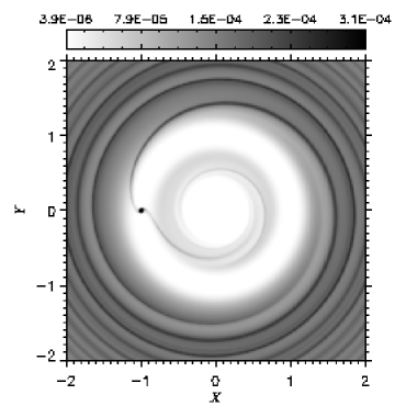
Figure 1: Global surface density around a $\mbox{$M_{\mathrm{p}}$}=1\,\mbox{$M_{\mathrm{J}}$}$ planet orbiting in a low-mass disk (see section 2.4.1). The density is shown after $370$ orbits, when the planet has migrated for $70$ orbits. In the linear grey-scale, at $5.2\,\mbox{{AU}}$, $\Sigma=10^{-4}$ corresponds to $32.9\,\mbox{$\mathrm{g}\,\mathrm{cm}^{-2}$}$.

Figure 2: Convergence tests regarding different configurations of Jupiter-mass models orbiting in a two-dimensional low-mass disc. Upper-left. Non-accreting planet with gravitational potential softening $\varepsilon=0.4\,\mbox{$R_{\mathrm{H}}$}$. Upper-right. Non-accreting planet with $\varepsilon=0.2\,\mbox{$R_{\mathrm{H}}$}$. Lower-left. Non-accreting planet with $\varepsilon=0.1\,\mbox{$R_{\mathrm{H}}$}$. Lower-right. Accreting planet with $\varepsilon=0.1\,\mbox{$R_{\mathrm{H}}$}$. The release time is equal to $100$ orbits, except for the accreting model for which $t_{\mathrm{rls}}=300$ orbits. Each panel shows how the semi-major axis, $a$, evolves when all torques from within the planet’s Hill sphere are taken into account (upper curves) and when the contribution of those torques arising inside of $0.5\,\mbox{$R_{\mathrm{H}}$}$ from the planet are neglected (lower curves). See text for further details.

Convergence tests were carried out on each of the low-mass disc models described in Section 2.4.1. The resolution was progressively increased by employing the grid systems 2D3G, 2D4G, and 2D5G (see Table 1). The last two grid systems, compared to the first, provide a linear resolution gain of a factor $2$ and $4$, respectively. For comparison purposes, we set the release time to $t_{\mathrm{rls}}=100$ orbits, except for the simulations concerning the accreting model that have $t_{\mathrm{rls}}=300$ orbits. The overall surface density from one of such calculations is displayed in Figure 1.

Figure 3: Surface density profile along the azimuthal position ($\phi=\phi_{\mathrm{p}}$) of a $\mbox{$M_{\mathrm{p}}$}=1\,\mbox{$M_{\mathrm{J}}$}$ planet, after $100$ orbital periods, orbiting in a low-mass disc. Different line types indicate models with different values of the gravitational potential softening: $\varepsilon=0.1\,\mbox{$R_{\mathrm{H}}$}$ (solid line); $\varepsilon=0.2\,\mbox{$R_{\mathrm{H}}$}$ (short-dash line); $\varepsilon=0.4\,\mbox{$R_{\mathrm{H}}$}$ (dash-dot line); accreting planet (long-dash line). If $a_{0}=5.2\,\mbox{{AU}}$ and $\mbox{$M_{*}$}=1\,\mbox{$M_{\sun}$}$, $\Sigma=10^{-4}$ corresponds to $32.9\,\mbox{$\mathrm{g}\,\mathrm{cm}^{-2}$}$.

Figure 2 shows that we achieved numerical convergence in all cases, with either accreting or non-accreting planets and with different values of $\varepsilon$. In some panels, the outcomes produced by the two grid systems can be hardly distinguished. The main numerical difficulty with the evaluation of gravitational torques arising from the coorbital region is related to the presence of large density gradients (Nelson & Benz, 2003b). Moreover, the shorter the smoothing length, the larger such gradients are. Figure 3 shows that there is an order-of-magnitude difference between the density peaks of the models with $\varepsilon=0.1\,\mbox{$R_{\mathrm{H}}$}$ and $\varepsilon=0.4\,\mbox{$R_{\mathrm{H}}$}$. For the $\varepsilon=0.1\,\mbox{$R_{\mathrm{H}}$}$ case, using the grid system 2D3G would mean that $\varepsilon$ was resolved by less than $2$ grid zones and, thus, the density gradients could be resolved too poorly. Therefore, we used the grid systems 2D4G and 2D5G for this case.

We also investigated whether there are any differences between simulations starting with or without an initial density gap (see section 2.4). Provided that the system is allowed to evolve for a sufficiently long time in order that the gap becomes deep enough ($\approx 500$ orbits), the migration behaviour is very similar to that of models initiated with a density gap.

Two sets of lines are displayed in each panel of Figure 2. These are intended to address the lingering question of the importance of torques exerted by matter residing deep inside the planet’s Hill sphere (D’Angelo et al., 2003; Bate et al., 2003). Thus, two configurations were simulated, differing only in whether or not torques within a radius $\beta\mbox{$R_{\mathrm{H}}$}$ from the planet are included in the calculation of the gravitational force in equations (8) and (9). In one configuration, all torques are taken into account (i.e., $\beta=0$). In the second configuration, the simulations were repeated neglecting the contribution of material lying inside the inner half of the Hill sphere (i.e., $\beta=0.5$). The choice $\beta=0.5$ was made to avoid the region where the density gradient is largest (see Fig. 3) and which mostly contains material orbiting the planet before it is released (see Fig. 4).

The streamlines in Figure 4 are constructed by integrating the velocity field $(u_{r},u_{\phi})$ at an instant in time. Strictly speaking, this procedure is in error for a migrating planet (right panels), as it moves during the interval of integration. But provided the planet moves only a small fraction of its Hill sphere over the integration time, the streamlines obtained are reasonably accurate. This condition is satisfied for the streamlines plotted in this Figure. It is of course incorrect to ignore torques from within the Hill sphere since material can move into or out of it (see Fig. 3) and the angular momentum associated with this mass flux is lost instead of being transferred to the planet’s orbit. Therefore, migration rates obtained from configurations with $\beta>0$ are not fully consistent from a physical standpoint, unless one can assure that the neglected material is constantly and not temporarily orbiting the planet.

In all cases we considered, the $\beta=0$ calculations resulted in slower migration and, thus, these results appear as the upper curves in each panel of Figure 2. We note that even when torques coming from material within the Hill sphere are included, numerical convergence is still achieved. This last point turns out to be crucial when high-mass discs are considered (see section 5).

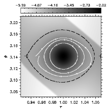
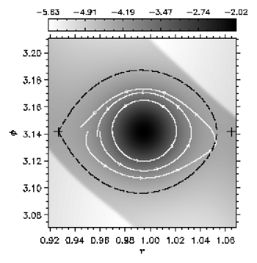
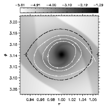
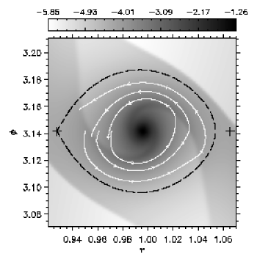
Figure 4: Surface density and streamlines around Jupiter-mass, non-accreting planets orbiting in a low-mass disc ($\mbox{$M_{\mathrm{D}}$}=0.01\,\mbox{$M_{\sun}$}$ within $26\,\mbox{{AU}}$). The results were obtained from computations executed with the grid system 2D4G (linear resolution $\mbox{$R_{\mathrm{H}}$}/\Delta r=38$) and softening $\varepsilon=0.4\,\mbox{$R_{\mathrm{H}}$}$ (top) and $0.1\,\mbox{$R_{\mathrm{H}}$}$ (bottom). The panels illustrate the situation at the release time $t=300$ orbital periods (left) and $50$ orbits later (right), while the planet is migrating. The grey-scale is logarithmic and, at $5.2\,\mbox{{AU}}$, $\Sigma=10^{-3}$ corresponds to $329\,\mbox{$\mathrm{g}\,\mathrm{cm}^{-2}$}$. The two streamlines closest to the planet start from distances of $\approx 0.36$ and $\approx 0.5\,\mbox{$R_{\mathrm{H}}$}$, respectively.

4.2 Three-dimensional simulations

Figure 5: Three-dimensional simulations of Jupiter-mass models (grid system 3D3G) orbiting in a low-mass disc, compared to analogous two-dimensional models (grid system 2D3G). Left. Non-accreting planet with gravitational potential softening $\varepsilon=0.4\,\mbox{$R_{\mathrm{H}}$}$. Centre. Non-accreting planet with $\varepsilon=0.2\,\mbox{$R_{\mathrm{H}}$}$. Right. Accreting planet with $\varepsilon=0.1\,\mbox{$R_{\mathrm{H}}$}$. The release time is equal to $100$ orbits for the non-accreting models and $300$ orbits for the accreting models. In each panel, the slower migration occurs with the configuration executed with $\beta=0$, whereas the faster migration occurs with the configuration run with $\beta=0.5$.

The vertical stratification of the flow variables in (vertically isothermal) discs does not play an important role in determining the strength of Lindblad torques acting on Jupiter-mass planets, provided that $\mbox{$R_{\mathrm{H}}$}\gtrsim H$ (Kley et al., 2001). However, since the flow structure around the Hill sphere of the planet is fully three-dimensional (D’Angelo et al., 2003; Bate et al., 2003), the amount of angular momentum delivered by material in the vicinity of the planet may be affected by the vertical motion of the fluid. We attempted to investigate this issue by means of 3D calculations (grid system 3D3G), whose results are shown in Figure 5. As for 2D computations, the effects of torques exerted by material within the Hill sphere were measured by running models with $\beta=0$ and $\beta=0.5$. In each panel of Figure 5, the evolution of the semi-major axis (solid lines) is compared to that obtained from 2D models (dashed lines) having an analogous grid system (2D3G). We were unable to test for convergence of the 3D calculations due to computational limitations (simulations with a factor $2$ increase in linear resolution would have required around $5000$ CPU hours each). But since the 2D calculations were converged, we speculate that at the same resolution 3D calculations are also converged because the density structure around and inside the Hill sphere is smoother in three dimensions.

Figure 5 shows that the two- and three-dimensional results are similar in the non-accreting cases. The Hill spheres of non-accreting planets contain more material in 3D than they do in 2D (see Fig. 6). Therefore, it is reasonable to expect that the migration is slightly faster in three dimensions.

The situation appears more complex in the accreting case, for which migration is slower in 3D than in 2D if $\beta=0.5$, but it is faster if $\beta=0$ (Fig. 5, right panel). Since the mass inside the Hill sphere is nearly the same in the two geometries (Fig. 6, bottom panel), we ascribed this discrepancy to the strong spiral waves that occur in the two-dimensional accreting calculations (Lubow et al., 1999; D’Angelo et al., 2002) which are much weaker in three-dimensions due to the possibility of vertical motions. Strong spiral waves do not develop when $\varepsilon$ is a fair fraction of $R_{\mathrm{H}}$. The non-accreting models with $\varepsilon=0.4$ and $0.2\,\mbox{$R_{\mathrm{H}}$}$ present a nearly featureless density structure close to the planet in both geometries, hence the similarity of the migration rates.

Figure 6: Mass enclosed within the Hill sphere of a $\mbox{$M_{\mathrm{p}}$}=1\,\mbox{$M_{\mathrm{J}}$}$ planet, as measured in 2D (circles) and 3D (diamonds) calculations. Top. Non-accreting model with $\varepsilon=0.4\,\mbox{$R_{\mathrm{H}}$}$. Centre. Non-accreting model with $\varepsilon=0.2\,\mbox{$R_{\mathrm{H}}$}$. Bottom. Accreting model with $\varepsilon=0.1\,\mbox{$R_{\mathrm{H}}$}$. Whether or not a gap is imposed on the initial density structure, the amount of material within the Hill sphere tends toward the same value.

Finally, we note that non-accreting 3D migration rates with $\varepsilon=0.4$ or $0.2\,\mbox{$R_{\mathrm{H}}$}$ are very similar. This suggests that no large variations should be expected if smaller values of $\varepsilon$ were employed, provided that a sufficiently refined mesh is utilised ($\Delta R=R\,\Delta\phi\ll\varepsilon$). The same conclusion seems to be valid in two dimensions, as discussed more quantitatively in the next section.

4.3 Migration rates: a quantitative analysis

So long as the semi-major axis does not change significantly (i.e., it remains of the same order of magnitude), the migration of a Jupiter-mass planet roughly follows an exponential decay (Nelson et al., 2000). We assume that even when the action of torques arising from corotation regions and from material orbiting the planet are included, the evolution of $a$ can also be described by an exponential decay law

$$a(t)=a_{0}\,e^{-(t-t_{\mathrm{rls}})/\tau_{\mathrm{M}}},$$ (12)

for times $t\geq t_{\mathrm{rls}}$. We take the migration time-scale $\tau_{\mathrm{M}}=a/|\dot{a}|$ to be a constant over the simulated time-interval of the actual planet’s migration (between $40$ and $100$ orbits). This simple parameterisation of $a=a(t)$ is very useful because $\tau_{\mathrm{M}}$ can be directly connected to the acting torques. In fact, if the orbit eccentricity is negligible then the conservation of the orbital angular momentum leads to the relation

$$\dot{a}=\frac{2\,\boldsymbol{\mathcal{T}}\boldsymbol{\cdot}\mathbf{\Omega}}{\mbox{$M_{\mathrm{p}}$}\,a\,\Omega^{2}},$$ (13)

in which the vector $\boldsymbol{\mathcal{T}}$ denotes the total external torque. This expression is commonly used to evaluate $\dot{a}$ from the vertical component of $\boldsymbol{\mathcal{T}}$ (which we simply indicate as $\mathcal{T}$), when a planet moves on a static orbit (i.e., it is not allowed to migrate).

We obtained estimates of $\tau_{\mathrm{M}}$ for all of the 2D models (grid system 2D4G) by performing a linear least-mean-squared fit of the relation $\ln{(a/a_{0})}=-(t-t_{\mathrm{rls}})/\tau_{\mathrm{M}}$. The results are listed in the second and third columns of Table 3, labelled as “moving” migration time-scale. The relative error on each estimate is at most $10^{-3}$ and only for this reason $\tau_{\mathrm{M}}$ is given with three significant digits. Discrepancies between estimates computed from 2D and 3D non-accreting models are below $\sim 10$ per cent. Since the accreting models present a more significant discrepancy, $\tau_{\mathrm{M}}$ is also reported for the simulations in three dimensions.

Including the effect of matter orbiting the planet tends to slow down its inward drifting motion, regardless of the employed disc geometry, as clearly indicated in Figure 5. The comparison between the $\beta=0$ and $\beta=0.5$ migration time-scales shows that the torque from this material can be comparable to that from corotation and Lindblad resonances. The total (positive) torque produced inside the inner half of the Hill sphere is

$$\mathcal{T}_{\mathrm{HS}}=\mathcal{T}-\mathcal{T}_{\mathrm{LC}}\propto\frac{1}{\tau_{\mathrm{M}}[\beta=0]}-\frac{1}{\tau_{\mathrm{M}}[\beta=0.5]},$$ (14)

whereas the magnitude of the total (negative) torque exerted from the rest of the disc (i.e., Lindblad and corotation torques), $\left|\mathcal{T}_{\mathrm{LC}}\right|$, is proportional to $1/\tau_{\mathrm{M}}[\beta=0.5]$. Hence, the ratio between the two contributions is

$$\frac{\mathcal{T}_{\mathrm{HS}}}{\left|\mathcal{T}_{\mathrm{LC}}\right|}=1-\frac{\tau_{\mathrm{M}}[\beta=0.5]}{\tau_{\mathrm{M}}[\beta=0]}.$$ (15)

Entries in the second and third columns of Table 3 indicate that in the model with softening $\varepsilon=0.4\,\mbox{$R_{\mathrm{H}}$}$ the material close to the planet accounts for a relatively small contribution ($22$ per cent). However, shorter smoothing lengths dramatically increase the torque ratio, which becomes greater than $60$ per cent in the non-accreting models with $\varepsilon=0.2\,\mbox{$R_{\mathrm{H}}$}$ and $0.1\,\mbox{$R_{\mathrm{H}}$}$. A similar ratio between torques is obtained in the 3D accreting model.

These migration time-scales can be compared with the Type I (no gap, resonant) time-scale of about $4\times 10^{2}$ orbits in 2D and $6\times 10^{2}$ orbits in 3D (Tanaka et al., 2002) and the Type II (viscous) time-scale $2\,a^{2}/(3\,\nu)\simeq 10^{4}$ orbits.

Note that the 2D migration rates tend to converge as $\varepsilon$ is decreased. In particular, the migration rates for $\varepsilon=0.2\,\mbox{$R_{\mathrm{H}}$}$ and $0.1\,\mbox{$R_{\mathrm{H}}$}$ differ by less than $10$ per cent.

4.4 Comparison of migration rates of static and migrating planets: the Jupiter-mass case

Table 3: Comparison of static and moving migration time-scales for a Jupiter-mass planet in a low-mass disc.

	Moving		Static
$\varepsilon$	$\beta=0$	$\beta=0.5$	$\beta=0$	$\beta=0.5$
$0.4\,\mbox{$R_{\mathrm{H}}$}^{\phantom{{\dagger}}}$	$9.94\times 10^{3}$	$7.75\times 10^{3}$	$1.0\times 10^{4}$	$7.8\times 10^{3}$
$0.2\,\mbox{$R_{\mathrm{H}}$}^{\phantom{{\dagger}}}$	$1.76\times 10^{4}$	$6.34\times 10^{3}$	$1.8\times 10^{4}$	$6.2\times 10^{3}$
$0.1\,\mbox{$R_{\mathrm{H}}$}^{\phantom{{\dagger}}}$	$1.51\times 10^{4}$	$5.71\times 10^{3}$	$1.8\times 10^{4}$	$5.7\times 10^{3}$
$0.1\,\mbox{$R_{\mathrm{H}}$}^{{\dagger}}$	$5.97\times 10^{4}$	$4.86\times 10^{3}$	$4.8\times 10^{4}$	$4.2\times 10^{3}$
$0.1\,\mbox{$R_{\mathrm{H}}$}^{{\ddagger}}$	$1.54\times 10^{4}$	$5.77\times 10^{3}$	$1.5\times 10^{4}$	$5.4\times 10^{3}$
† 2D accreting model. ‡ 3D accreting model.

The migration time-scales labelled as “moving” refer to the time-scale, $\tau_{\mathrm{M}}$, in equation (12) and were computed as explained in Section 4.3. They are expressed in units of initial orbital periods, i.e., $11.9$ years if $a_{0}=5.2\,\mbox{{AU}}$. One-standard deviation uncertainties for these estimates range from $1$ to $10$ orbits. See Section 4.1 for an explanation of configurations $\beta=0$ and $\beta=0.5$. Migration time-scales labelled as “static” were determined from equation (13) by employing torques averaged over the last ten orbits before the release time. Computations were executed with the grid system 2D4G.

We examined whether the torque exerted on the planet by the disc material is influenced by the radial motion of the planet. As discussed in Section 1, the motion of the planet might be able to affect the coorbital torques and therefore the migration rate. In order to test this hypothesis, we computed the total torque acting on the planet during the last ten orbital periods before it was released. This was done for both $\beta=0$ and $\beta=0.5$ configurations. Since no angular momentum is actually extracted from or added to the planetary orbit, which thus remains static, we shall refer to such torques as static torques. The migration time-scales listed in the two right-most columns of Table 3 were obtained from the average static torques by using equation (13). In Table 3 we compared these “static” migration time-scales, $\tau_{\mathrm{M}}^{\mathrm{S}}$, with the migration time-scales, $\tau_{\mathrm{M}}$, measured from the moving planet calculations. In all cases, there is close agreement between the static and moving migration time-scales. These results show that under these circumstances of disc and planetary masses, there is no strong dependence of the torques on whether planets are on fixed orbits or allowed to migrate.

5 Results of high-mass disc models

The Type II migration rate depends only on the viscous time-scale of the disc near the location of the planet and is independent of the disc density, provided that the gap is devoid of material. Yet gaps are generally not completely cleared and the Type II time-scale prediction does not take into consideration the angular momentum exchanged between the planet and the “gap” material. Some of this material travels on horse-shoe orbits, while other material circulates within the planet’s Hill sphere. The angular momentum delivered in either case may play a major role in planetary migration (see, e.g., Masset, 2001) and it is proportional to the local mass density. In fact, MP03 recently claimed that there exists a critical mass (when the material around the planet is more massive than the planet), beyond which a runaway migration process sets in.

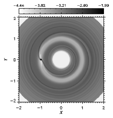
Figure 7: Global surface density around a $\mbox{$M_{\mathrm{p}}$}=0.3\,\mbox{$M_{\mathrm{J}}$}$ (non-accreting) planet orbiting in a $0.024\,\mbox{$M_{\sun}$}$ disk. The density is displayed at $t=550$ orbits, when the planet has migrated for about $70$ orbits. The grey-scale is logarithmic and $10^{-3}$ corresponds to $329\,\mbox{$\mathrm{g}\,\mathrm{cm}^{-2}$}$, at $5.2\,\mbox{{AU}}$. The average gap density is $2.5\times 10^{-4}$ or $82\,\mbox{$\mathrm{g}\,\mathrm{cm}^{-2}$}$.

We ran simulations of Saturn-like bodies ($\mbox{$M_{\mathrm{p}}$}=0.3\,\mbox{$M_{\mathrm{J}}$}$) embedded in a disc as massive as $24\,\mbox{$M_{\mathrm{J}}$}$ inside $13\,\mbox{{AU}}$. The annular region within $2\,\mbox{$R_{\mathrm{H}}$}$ from the planet is initially $7.5$ as massive as the planet. Nonetheless, the aspect ratio is small enough ($H/r=0.03$) so the thermal condition for gap formation, $\mbox{$M_{\mathrm{p}}$}/\mbox{$M_{*}$}>3\,(H/r)^{3}$ (e.g., Lin & Papaloizou, 1993), is fulfilled and therefore the migration might be within the Type II regime, although the gap is not completely cleared as can be seen in Figure 7. In these cases, with massive discs and small aspect ratios, very large density gradients develop inside the Hill sphere. Therefore, it is especially important to investigate the dependence of the results on numerical resolution. We achieved convergence for the flow outside of the Hill sphere by using numerical resolutions of order $13$ grid zones per Hill radius. However, in order to accurately determine the contributions to the migration rate from material inside the Hill sphere, resolutions higher than $52$ grid zones per Hill radius are necessary.

5.1 Convergence tests

Figure 8: Computations of a Saturn-mass planet orbiting in a high-mass disc: convergence tests. The gravitational potential softening, $\varepsilon$, is $60$ per cent of the local disc scale-height. The release time is equal to $477$ orbits. The left panel shows the evolution of $a$ when all torques are taken into account (i.e., $\beta=0$). The right panel shows how the evolution of the semi-major axis proceeds when the contribution of those torques arising from inside the Hill sphere (i.e., $\beta=1.0$) are neglected . The dot-dash line (labelled as 2D1Gb) refers to a calculation executed with the same numerical resolution as in MP03.

As mentioned in Section 2.4.2, the model setup and the disc parameters were chosen to match as closely as possible those in MP03. The smoothing length was $60$ per cent of the local disc thickness, $H$, (i.e., $\varepsilon=0.3878\,\mbox{$R_{\mathrm{H}}$}$), the planet was non-accreting, and $t_{\mathrm{rls}}=477$ orbits. We performed a calculation using a single-level grid (2D1Gb, see Table 2) aimed at reproducing the resolution used by MP03 ($\Delta r/\mbox{$R_{\mathrm{H}}$}\simeq 0.3$ and $\Delta r/\varepsilon\simeq 0.8$). We then performed a convergence test using different numerical resolutions, as provided by the grid systems 2D3Gb, 2D4Gb, and 2D5Gb (see Table 2). An additional convergence test, involving the grid system 2D6Gb, is discussed in Section 5.1.1.

The left panel of Figure 8 shows the outcomes of the tests for the evolution of the semi-major axis concerning the configuration with $\beta=0$. The dot-dash line in this panel represents the result from the single-grid computation 2D1Gb, which should be compared to the model labelled as $\mathrm{S}_{8}$ in Figure 2 of MP03. Given the remarkable agreement between our and their outcome, we are confident that we reproduced the same physical and numerical conditions for runaway migration. Yet, computations repeated with finer and finer resolutions gave smaller and smaller migration rates which, as displayed in Figure 8 (left panel), failed to converge. The gain in linear resolution achieved (over the single-grid simulation) with the employed grid systems ranges from $4$ (2D3Gb) to $16$ (2D5Gb). In the highest resolution models, there are $52$ grid zones per Hill radius. Comparing the short-dash and dot-dash curves in left panel of Figure 8, one realises that the average migration speed obtained over the first $25$ orbits with the grid system 2D3Gb is only half (in physical units, $\langle\dot{a}\rangle\approx-5\times 10^{-3}\,\mbox{{AU}}\,\mathrm{yr}^{-1}$) of that in MP03. Calculations executed with the grid systems 2D4Gb and 2D5Gb give even lower migration speeds of $\langle\dot{a}\rangle\simeq-5\times 10^{-4}$ and $-1.4\times 10^{-4}\,\mbox{{AU}}\,\mathrm{yr}^{-1}$, respectively.

While there is a factor of $10$ decrease in disc torques acting on the planet in going from grid systems 2D3Gb to 2D4Gb, this factor reduces to $3.6$ when the two most refined grid systems are considered. Yet, from the behaviour of semi-major axis evolution shown in the left panel of Figure 8, we cannot determine whether it is converging. To assess this point we employed the grid system 2D6Gb (see section 5.1.1) which indicates that the solid line in Figure 8 is basically a converged evolution.

Figure 9: Mass enclosed within the Hill sphere of a $\mbox{$M_{\mathrm{p}}$}=0.3\,\mbox{$M_{\mathrm{J}}$}$ planet, as measured from simulations with increasing resolutions: single-level grid 2D1Gb (asterisks); grid system 2D3Gb (diamonds); grid system 2D4Gb (squares); grid system 2D5Gb (circles).

Figure 10: Surface density profile at the azimuthal position of a planet with $\mbox{$M_{\mathrm{p}}$}/\mbox{$M_{*}$}=3\times 10^{-4}$, after $450$ orbital periods (the planet starts migrating at $t_{\mathrm{rls}}=477$ orbits), orbiting within a high-mass disc. Different line types refer to computations performed with different grid systems: 2D5Gb (solid line); 2D4Gb (long-dash line); 2D3Gb (short-dash line). If $a_{0}=5.2\,\mbox{{AU}}$ and $\mbox{$M_{*}$}=1\,\mbox{$M_{\sun}$}$, $\Sigma=10^{-2}$ is equal to $3.29\times 10^{3}\,\mbox{$\mathrm{g}\,\mathrm{cm}^{-2}$}$.

The right panel in Figure 8 shows the semi-major axis evolution from the same calculations as in the left panel but executed with $\beta=1.0$, i.e., excluded torques arising inside the planet’s Hill sphere. As before, this choice of $\beta$ was made to exclude the region around the planet with largest density gradients as well as largest torque densities. Clearly, numerical convergence was readily achieved with this configuration. The migration time-scale, obtained from a least-mean-squared fit to the data (see section 4.3), is $\tau_{\mathrm{M}}=493$ orbits. Furthermore, outcomes of simulations executed with $\beta=0.75$ attained convergence at almost the same rate of migration as with $\beta=1.0$. Therefore, we conclude that the material close to the planet must be held responsible for the non-convergence of the $\beta=0$ configuration in the left panel of Figure 8. That is, the torque arising from within the Hill sphere converges very slowly with increasing resolution. Despite the fact that the amount of material inside the planet’s Hill sphere increases as the grid resolution is raised (see Fig. 9), the resulting migration rates or net torques are actually smaller. Figure 10 shows the surface density near the planet at an advanced time, shortly before it is allowed to migrate. We note that the mass near the planet seems to be converging at the highest resolutions, but convergence is not yet formally achieved. This Figure also implies that most of the material is piled up very close to the planet. We measured that $80$ per cent of the mass contained inside the Hill sphere is concentrated within a distance of $0.2\,\mbox{$R_{\mathrm{H}}$}$ from the planet.

The mass build up within the Hill sphere appears to suggest that disc self-gravity may be dynamically important. However, this may not actually be the case. A simple calculation of a viscous disc that accretes at the typical rates of $10^{-8}\,\mbox{$M_{\sun}$}$ per year suggests that it is likely not self-gravitating (the value of the Toomre parameter $Q$ is much greater than unity for the parameters in this paper). In the simulations presented here, the mass build up is concentrated in a region of order the smoothing length (see Fig. 10). Within that radius, further inward viscous accretion is artificially slow because the gravitational potential of the planet tends to enforce rigid rotation (see second term in eq. [6]). In addition, the boundary condition of no accretion on the planet prevents the accumulated gas from being removed from the simulation. As such, much of the gas accumulated within a smoothing length represents material that is incorporated by the planet, rather than residing in the disc.

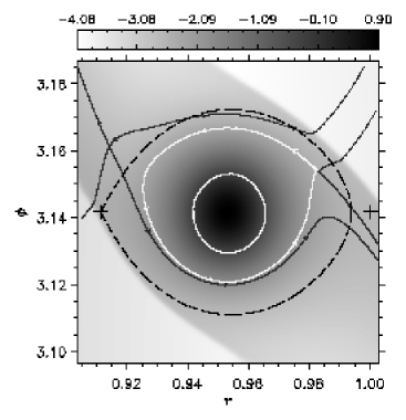
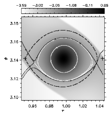
Figure 11: Surface density and streamlines around a $\mbox{$M_{\mathrm{p}}$}=0.3\,\mbox{$M_{\mathrm{J}}$}$, non-accreting planet orbiting in a high-mass disc ($\mbox{$M_{\mathrm{D}}$}=0.024\,\mbox{$M_{\sun}$}$ within $13\,\mbox{{AU}}$). The dashed line indicates the Roche lobe and the crosses mark the position of the L1 and L2 Lagrange points. The top-left panel refers to the time $t=450$ orbital periods (i.e., before it is released) whereas the top-right panel displays the situation at $t=497$ orbits with the configuration $\beta=1.0$ (its instantaneous radial speed is $\dot{a}\simeq-1.5\times 10^{-4}\,\mbox{{AU}}\,\mathrm{yr}^{-1}$). The bottom panel refers to the same time but when all torques are taken into account (i.e., $\beta=0$). The grey-scale is logarithmic and, at $5.2\,\mbox{{AU}}$, $10^{-3}$ corresponds to $329\,\mbox{$\mathrm{g}\,\mathrm{cm}^{-2}$}$. These results were obtained from computations executed with the grid system 2D5Gb (linear resolution $\Delta r/\mbox{$R_{\mathrm{H}}$}\simeq 2\times 10^{-2}$). As in Figure 4, the streamlines in the bottom panel do not account for the planet’s motion because of the small $\dot{a}$. A more strict procedure was instead employed to calculate the streamlines in the top-right panel. In this case we integrated the velocity field $(u_{r}-\dot{a},u_{\phi})$, where $\dot{a}$ is the instantaneous radial speed of the planet.

Although the configuration with $\beta=1.0$ provides numerically converged migration rates, one has to be wary of their physical meaning. Figure 11 illustrates that before the planet is released (top-left panel) material on horse-shoe orbits passes through the Roche lobe as close to the planet as $\approx 0.5\,\mbox{$R_{\mathrm{H}}$}$. Yet, if the planet starts rapidly migrating this picture is bound to change. The top-right panel shows a snapshot after $20$ orbits from the release time, as the planet radially moves at a speed $\dot{a}\simeq-1.5\times 10^{-4}\,\mbox{{AU}}\,\mathrm{yr}^{-1}$ (configuration $\beta=1.0$ and grid system 2D5Gb). The situation appears less symmetric than before the release and the flow structure within the Hill sphere has been altered by the rapid planetary motion. As a reference, we also show in the bottom panel what happens when all torques are consistently taken into account ($\beta=0$). We calculated the torques arising from the Hill sphere in the situation depicted in the top-right panel and we found that they are three times as large (and more positive) as those exerted, at the same time, in the configuration $\beta=0$ (bottom panel). This difference may indicate that the faster motion in the $\beta=1$ case has artificially changed the density distribution inside the Hill sphere and thus the circulation in the coorbital region.

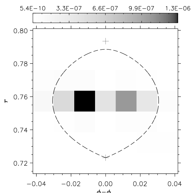
Figure 12: Left. Absolute value of the torque density (linear scale) close to a planet with $\mbox{$M_{\mathrm{p}}$}/\mbox{$M_{*}$}=3\times 10^{-4}$ and orbiting in a high-mass disc. The dashed line indicates the Roche lobe and the crosses mark the L1 and L2 Lagrange points. This calculation was executed with the single-level grid 2D1Gb ($\Delta r\simeq 0.3\,\mbox{$R_{\mathrm{H}}$}$). Shaded pixels represent the actual size of the grid zones. The torque distribution is illustrated at $t=496$ orbital periods while the planet is migrating at an average rate $\langle\dot{a}\rangle\approx-10^{-2}\,\mbox{{AU}}\,\mathrm{yr}^{-1}$. The torque density is negative when $\phi<\phi_{\mathrm{p}}=\pi$ and positive when $\phi>\phi_{\mathrm{p}}$. It is evident that at such low resolution there is an unbalanced inward torque that is not observed in higher resolution calculations (see top panels of Fig. 13). Right. The solid line shows the profile of the absolute value of the torque density (shown in the left panel) through the radial position of the planet. The filled circles indicate the positions of the data. The dashed line refers to an analogous profile from the highest resolution calculation (grid system 2D5Gb), which was rescaled so that its maximum value was $1.3\times 10^{-6}$.

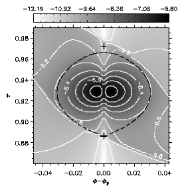
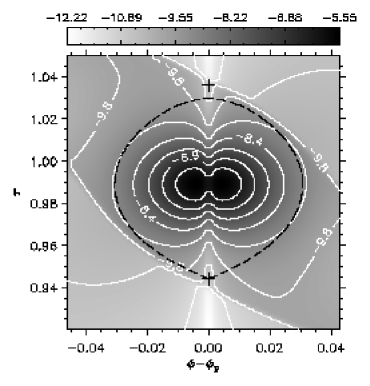
Figure 13: Top. Absolute value of the torque density (logarithmic scale) and contour lines around and inside the Hill sphere of a planet with $\mbox{$M_{\mathrm{p}}$}/\mbox{$M_{*}$}=3\times 10^{-4}$, orbiting in a high-mass disc. The snapshots are taken at $t=537$ orbital periods, i.e., after the planet has migrated for $60$ orbits. The left panel refers to the calculation executed with the grid system 2D4Gb while the right panel refers to that executed with the grid system 2D5Gb. The torque density is negative when $\phi<\phi_{\mathrm{p}}$ and positive when $\phi>\phi_{\mathrm{p}}$. Note that the torque density at the planet position is not exactly zero because the planet does not sit on the centre of a mesh zone, where density torque is computed. Bottom. The left panel shows the cut of the torque density magnitude through the planet’s radial position for the models shown in the top panels. The solid line represents the outcome of the higher resolution simulation (2D5Gb) whereas the dashed line corresponds to the lower resolution simulation (2D4Gb). The ratio between these two curves (higher to lower resolution calculation) is displayed in the right panel. The profile appears asymmetric (with respect to $\phi-\phi_{\mathrm{p}}=0$) only towards the outer regions $|\phi-\phi_{\mathrm{p}}|>0.02\simeq 0.4\,\mbox{$R_{\mathrm{H}}$}/a$.

The reason for the very fast migration rate, measured at the lowest resolution (single-level grid 2D1Gb), can be understood by examining the two dimensional linear map of the torque density magnitude in the left panel of Figure 12. The plot describes the situation after $19$ orbits from the planet’s release, when it is migrating inwards at an average rate of roughly $10^{-2}\,\mbox{{AU}}\,\mathrm{yr}^{-1}$. The map clearly shows how the poor resolution (the grid zone size is indicated by the shaded pixels) cannot properly handle the large torque gradients within the Hill sphere and produces a very large differential torque. This resolution effect led to the vastly different migration time-scales between the lowest and highest curves in the left panel of Figure 8. A cut of the torque density magnitude, through the planet’s radial position, is shown in the right panel of Figure 12 for both the computation executed with the grid 2D1Gb (solid line) and that executed with the high-resolution grid system 2D5Gb (dashed line). The dashed-line profile was rescaled so that the maximum values were similar to those of the solid-line profile. The filled circles represent the actual data. The low-resolution torque density is highly asymmetric. The two maxima alone exert a negative torque that would result in a migration time-scale of $80$ orbits. The large mismatch between the torque density extrema is not observed in high-resolution model, in which their opposite sign contributions nearly cancel each other.

The differences between the two highest resolution calculations discussed here are less evident and require some discussion. Two-dimensional logarithmic maps of the magnitude of the torque density for such models are shown in the top panels of Figure 13. They were obtained from the computations with the grid systems 2D4Gb (left) and 2D5Gb (right). Both maps describe the situation $60$ orbits after the planet’s release. The torque density is positive on the side leading the planet, $\phi>\phi_{\mathrm{p}}$, and negative on the opposite side ($\phi<\phi_{\mathrm{p}}$). As clearly indicated in the Figure, the torque density within the inner half of the Hill sphere is orders of magnitudes larger than it is anywhere else in the surrounding region and, therefore, in the whole disc. This is the reason why the migration speed is so susceptible to the torques exerted within the planet’s Hill lobe. Any mismatch between the positive ($\phi>\phi_{\mathrm{p}}$) and negative ($\phi>\phi_{\mathrm{p}}$) contributions can produce a very large net (either positive or negative) torque acting on the planet. From the top panels in Figure 13, the torque density magnitude appears rather symmetric with respect to the direction $\phi=\phi_{\mathrm{p}}$. This is clear from the bottom-left panel, where cuts through the planet’s radial position are compared for the two grid systems. The solid line corresponds to the more resolved model. Nevertheless, the results shown in the bottom-left panel of Figure 8 imply that the torque exerted by the Hill sphere is more positive (i.e., greater than zero and larger) in the higher resolution model (grid system 2D5Gb) than it is in the lower resolution one (grid system 2D4Gb). Indeed, this effect is highlighted by the ratio between the two torque density cuts (solid to dashed profile, that is higher to lower resolution results) reported in the bottom-right panel of Figure 13. The important thing to note is that the curve is asymmetric, with respect to the direction $\phi=\phi_{\mathrm{p}}$, towards the the outer parts of the Hill sphere $|\phi-\phi_{\mathrm{p}}|>0.02\simeq 0.4\,\mbox{$R_{\mathrm{H}}$}/a$. This means that the mismatch between the positive ($\phi>\phi_{\mathrm{p}}$) and negative ($\phi<\phi_{\mathrm{p}}$) torques arising from the region $|\phi-\phi_{\mathrm{p}}|>0.02$ produces a net positive torque that is greater in the higher resolution model than it is in the lower resolution model. Most of the asymmetry, and therefore the discrepancy between the two computations, must be confined to the region enclosed between roughly $0.4\,\mbox{$R_{\mathrm{H}}$}$ and $0.75\,\mbox{$R_{\mathrm{H}}$}$ from the planet because convergence tests executed with the configuration $\beta=0.75$ gave the same migration behaviour for the two models.

We also performed 3D simulations, using the grid system 3D3Gb (see Table 2), yet no appreciable differences from 2D calculations executed with the grid system 2D3Gb were observed. This was easily predictable, given the large smoothing length adopted in these models and the very small the disc thickness.

5.1.1 A converged migration rate

Figure 14: Semi-major axis evolution (top) and migration speed (bottom) obtained from the grid system 2D6Gb (solid line) versus those calculated with grid systems 2D5Gb (long-dash line) and 2D4Gb (short-dash line). The units of $\dot{a}$ are initial Hill radii per orbit. In these simulations the release time was equal to $t_{\mathrm{rls}}=277$ orbits (see text). All torques are taken into account (i.e., $\beta=0$). This additional convergence test shows that the migration behaviour given by the grid system 2D5Gb is fundamentally a converged one.

In order to evaluate how close to convergence the orbital evolution given by the grid system 2D5Gb is (see Fig. 8, left panel), we made a final attempt and ran a model with the grid system 2D6Gb (see Table 2), which resolves the Hill radius with about $104$ grid zones. However, we could not run a complete model as those in Section 5.1. In fact, evolving a model for about $550$ orbits with such a grid system would have required around $8000$ CPU hours. We only had the computational resources to run this particular model for about $292$ orbital periods. Therefore we set the release time to $t_{\mathrm{rls}}=277$ orbits and let the planet migrate for about $15$ orbits.

To carry out a consistent comparison, we performed calculations with the grid systems 2D4Gb and 2D5Gb imposing the same release time. The results are shown in Figure 14. Despite the short time over which the planet actually migrated, the highest resolution model (solid lines) provided evolutions of both $a$ (top panel) and $\dot{a}$ (bottom panel) that are in very good agreement with those computed with the grid system 2D5Gb (long-dash lines). This implies that the rates of migration obtained with the latter grid system (2D5Gb) can be considered as converged rates. This also indicates that in order to accurately compute torques from within and around the Hill sphere, in a configuration as described in Section 2.4.2, linear resolutions on the order of $52$ grid zones per Hill radius are required.

It has to be emphasised that, while for Jupiter-mass planets in low-mass discs torques were converged with respect to both the numerical resolution and the smoothing length of the planet’s potential (see section 4), in the present case we only examined convergence with respect to the numerical resolution.

5.2 Comparison of migration rates of static and migrating planets: the Saturn-mass case

We performed the same type of comparison, as done above, for the torques acting on a static and migrating planet. We considered both the configurations $\beta=0$ and $\beta=1.0$. These results were obtained from the calculation run with the grid system 2D4Gb ($26$ grid zones per Hill radius). Recall that with $\beta=1.0$, complete numerical convergence was attained with $13$ grid zones per Hill radius and therefore the same result is produced by the model executed with the grid system 2D5Gb. With $\beta=0$, convergence was presumably obtained only with this last grid system. Nonetheless, it is still of interest to investigate if migration times-scales depend on whether the planet is allowed to migrate or kept on a fixed orbit, with the grid system 2D4Gb, since it yields a larger migration rate.

Using the torques measured during the last ten orbits before the planet is released, by the same procedure outlined in Section 4.4, we obtained static migration time-scales of $\tau_{\mathrm{M}}^{\mathrm{S}}=770$ initial orbits for $\beta=0$ and $\tau_{\mathrm{M}}^{\mathrm{S}}=540$ initial orbits for $\beta=1.0$. Both values are remarkably close to those obtained when the planet is allowed to move: $\tau_{\mathrm{M}}=773$ and $\tau_{\mathrm{M}}=493$ initial orbits, respectively (see Fig. 8).

6 Discussion and Conclusions

We calculated the migration rates of planets embedded in discs. These calculations were performed in two and three dimensions, using a reference frame that corotates with the planet and a nested-grid code that can provide high resolution close to the planet while it migrates. The models span a variety of smoothing parameters for the potential and a variety of grid resolutions. Both accreting and non-accreting boundary conditions near the planet were considered. We were especially interested in whether torques from the coorbital region can lead to runaway migration, as reported in MP03.

In the case of a Jupiter-mass planet embedded a low-mass disc ($\mbox{$M_{\mathrm{D}}$}=0.01\,\mbox{$M_{\sun}$}$ within $26\,\mbox{{AU}}$), the planet opens a gap in which there is some flowing material. Numerical convergence was readily obtained (see Fig. 2). The torques arising from within the Hill sphere do make a contribution to the torque (up to $60$ per cent), but always in the sense of reducing the migration rate. The migration time-scales are numerically of order the Type II migration time-scale $2\,a^{2}/(3\,\nu)\simeq 10^{4}$ orbits (see Table 3) and much longer than the Type I time-scale of about $5\times 10^{2}$ orbits.

In the case of a Saturn-mass planet embedded in a high-mass disc ($\mbox{$M_{\mathrm{D}}$}=0.02\,\mbox{$M_{\sun}$}$ within $13\,\mbox{{AU}}$), the planet opens a less clean gap and is much more susceptible to the larger amount of material that resides in the coorbital region. Numerical convergence in this case was much more difficult to achieve when torques from within the Hill sphere were included. Convergence was more easily obtained when considering only torques from outside the Hill sphere (see Fig. 8). The reason is that the mass of gas flowing within the Hill sphere is larger than the mass of the planet. Any inaccuracies in the density structure near the planet (e.g., due to finite resolution) can lead to strong net torques (see Fig. 12 and Fig. 13). Although numerically converged, migration rates that do not account for torques from within the Hill sphere (or a large fraction of it) are artificially large (compare curves for grid system 2D5Gb in the left and right panels of Fig. 8). This also affects the flow structure around the planet and in the coorbital region (see Fig. 11). With increasing resolution, the gas mass within the Hill sphere increases, yet the migration rate decreases. In the case that the resolution was about equal to the smoothing length, which was $0.39\,\mbox{$R_{\mathrm{H}}$}$, the migration rate was very high, comparable to the Type I migration rate (as also found by MP03). However at the highest resolution we applied with a release time of $477$ orbits, which was sixteen times higher (in terms of linear resolution), the migration rate dropped dramatically by more than two orders-of-magnitude. Discrepancies between higher resolution calculations are more subtle and arise from the outer half of the Hill sphere (see Fig. 13). A calculation based on the grid system 2D6Gb, for which $\mbox{$R_{\mathrm{H}}$}/\Delta r=104$, indicates that accurately describing torques from around and inside the Hill sphere requires resolutions of at least $52$ grid zones per Hill radius. At highest resolution, the migration time-scale is about $3\times 10^{3}$ orbits (see left panel of Fig. 8), somewhat shorter than the Type II time-scale. But the process is unlikely to be simply described by Type II migration.

We calculated the torques exerted by the disc on planets whose orbits are fixed and used these to obtain migration time-scales. Comparing these time-scales to those obtained by releasing the planet and allowing it to migrate freely through the disc, we found no significant difference in the migration time-scales. This argues that the corotation torques are not greatly affected by the radial drift of a planet.

In summary, the migration rates for planets that open impure gaps (in which some material flows) are substantially smaller than Type I rates and do not seem to be simply described by Type II migration. Torques arising near the planet can be important, but do not appear to have a dramatic effect in raising the rates. Resolution is key to obtaining accurate torques.

Appendix A Numerical tests

The purpose of this Appendix is to demonstrate the reliability of the nested-grid technique when it is applied to disc-planet interaction calculations and, more specifically, to planetary migration. The capabilities of this technique in the context of astrophysical fluid-dynamics modelling have been addressed by a number of authors (e.g., Ruffert, 1992; Yorke, Bodenheimer & Laughlin, 1993; Yorke & Kaisig, 1995; Ziegler & Yorke, 1997, and references therein). We therefore concentrate on specific test computations that closely concern the application we did in this paper. The tests that we report here were done in two dimensions only to avoid excessively long computing times.

We set up a model of a Jupiter-mass planet ($\mbox{$M_{\mathrm{p}}$}/\mbox{$M_{*}$}=10^{-3}$) in a massive disc with $\mbox{$M_{\mathrm{D}}$}=1.1\times 10^{-2}\,\mbox{$M_{*}$}$ (inside $13\,\mbox{{AU}}$ of a $1\,\mbox{$M_{\sun}$}$ star) and whose aspect ratio is $H/r=0.03$. The initial surface density drops as $r^{-1/2}$ but it also includes a theoretical gap along the planetary orbit, as done for most of the Jupiter-mass models discussed so far. The adopted viscosity prescription was the same as that chosen for all the other calculations (see section 2.4.1). The radial extent of the computational domain ranges from $0.4$ to $2.5$ length units and reflective boundary conditions were applied to both edges of the disc to enforce mass conservation (the planet was not accreting). The planet’s orbit was initialised with $a_{0}=1$ (and with zero eccentricity) and it was kept steady for the first orbital period (i.e., $t_{\mathrm{rls}}=1$). The reference frame was set to rotate at a variable rate $\Omega=\Omega(t)$ so that $\phi_{\mathrm{p}}=\pi$ throughout the simulations, according to the procedure introduced in Section 2.3.

Figure 15: Semi-major axis evolution of the test model as calculated in a nested-grid mode with the grid system 2G (solid line) and in a single-grid mode with the grid 1G (dashed line). Radial and azimuthal resolutions ($\Delta r\simeq\Delta\phi\simeq 7.0\times 10^{-3}$) coincide over roughly a half of the whole computational domain ($[0.4,2.5]\times 2\,\pi$).

Figure 16: Top. Normalised difference of the two functions $a_{\mathrm{2G}}$ and $a_{\mathrm{1G}}$, shown in Figure 15, according to equation (A1). Each filled circle represents the average of the data over time-intervals of a tenth of an orbit that are centred at the middle point of each time-interval. Bottom. Running time average of the data displayed in the top panel, according to equation (A2).

In order to evaluate in quantitative terms the behaviour of the nested-grid technique, the model outlined above was executed with a two-level grid system (i.e., in nested-grid mode) as well as with a single-level grid (i.e., in single-grid mode). The first grid level of the two-level grid system (henceforth 2G), which covers the whole computational domain, had $N_{r}\times N_{\phi}=147\times 455$ grid zones ($\Delta r\simeq 1.46\times 10^{-2}$ and $\Delta\phi\simeq 1.40\times 10^{-2}$), whereas the second level had $N_{r}\times N_{\phi}=264\times 464$ zones ($\Delta r\simeq 7.3\times 10^{-3}$ and $\Delta\phi\simeq 7.0\times 10^{-3}$). With this setup, the higher resolution region extends from $r\simeq 0.5$ to $r\simeq 2.4$ and from $\phi\simeq\pi/2$ to $\phi\simeq 3\,\pi/2$. In order to achieve the same resolution with a single-level grid (henceforth 1G), the mesh must have $N_{r}\times N_{\phi}=290\times 904$ grid zones. Although the grid system 2G covers nearly a half of the whole domain with the same numerical resolution as the grid 1G, the perturbations induced by the planet propagate to the entire disc over a short time-scale and after $5$ orbits the spiral wave pattern has already developed. Therefore, after a few orbits, one should expect that the results of the two simulations start to differ. The discrepancy depends upon the ability of the first level of the grid 2G to capture the same flow features as the grid 1G does, in the region $\phi<\pi/2$ and $\phi>3\,\pi/2$.

Since this study is about migration, we focused on the evaluation and comparison of the semi-major axis evolutions, which also give a direct indication of the acting torques as a function of time. Note that this is a more strict test than simply comparing the torque distributions at certain times, which would only imply that $\dot{a}$ is the same at those times. The orbital decay for the two simulations is shown in Figure 15. The solid and dashed lines pertain to grids 2G and 1G, respectively. To estimate the differences in more detail, we computed the normalised difference

$$\frac{\Delta a}{\bar{a}}=2\left(\frac{a_{\mathrm{II}}-a_{\mathrm{I}}}{a_{\mathrm{II}}+a_{\mathrm{I}}}\right),$$ (A1)

where the labels $\mathrm{I}$ and $\mathrm{II}$ identify the used grids 1G and 2G, respectively. Since the time-step is different in the two simulations, $a_{\mathrm{1G}}$ and $a_{\mathrm{2G}}$ were averaged over time-intervals of $0.1$ orbits and the value measured from equation (A1) was assigned to the central time of each interval. As shown in the top panel of Figure 16, $\Delta a/\bar{a}$ is typically a few times $10^{-5}$ and it doesn’t increase beyond $1.5\times 10^{-4}$. The bottom panel of Figure 16 illustrates the running time average of the normalised difference

$$\left\langle\frac{\Delta a}{\bar{a}}\right\rangle_{t}=\frac{1}{t}\int_{0}^{t}\frac{\Delta a}{\bar{a}}\,\mathrm{d}t^{\prime},$$ (A2)

which indicates that the discrepancies in the orbital evolutions are on average around a few times $10^{-3}$ per cent.

From the viewpoint of the computational load, the advantage of the nested-grid technique is remarkable: in the computations reported above, the time-step required for numerical stability by grid 2G (first level) is twice as long as that required by grid 1G and so the time needed to complete one orbital period is twice as short. It is also worthwhile to point out that the refinement capabilities of the nested-grid strategy does not reduce the accuracy of the numerical algorithm, which strictly remains second-order accurate in space since the mesh step size is always constant on each grid level.

Figure 17: Comparison between the orbital evolutions computed with the grid 1G setting a constant rotation rate $\Omega=\Omega_{0}=\sqrt{G\,\mbox{$M_{*}$}/a^{3}_{0}}$ and a variable rate (i.e., $\dot{\Omega}\neq 0$) such that the planet’s azimuthal position remains constant. Top. Normalised difference (see eq. [A1]) sampled as in the top panel of Figure 16. Bottom. Running time average of the data displayed in the top panel.

For the sake of completeness, we show a test on the accelerated grid technique that we implemented and employed in this work. Other tests (not reported here) on the angular momentum conservation of both the disc and the planet proved that conservation was achieved down to the machine precision. Thus, we refer to a more relevant situation and show how the migration calculated in a reference frame rotating with a variable $\Omega$ compares to that calculated in a uniformly rotating grid with $\Omega=\Omega_{0}=\sqrt{G\,\mbox{$M_{*}$}/a^{3}_{0}}$. The outcome of such comparison is illustrated in Figure 17. We computed the normalised difference (top panel) and the running time average (bottom panel), where the quantity $a_{\mathrm{II}}$ in equation (A1) was obtained from the grid 1G with $\dot{\Omega}\neq 0$ while the quantity $a_{\mathrm{I}}$ was obtained from the grid 1G with static rotation (i.e., $\dot{\Omega}=0$). As Figure 17 proves, the discrepancy between the two semi-major axis evolutions is not significant. It has to be stressed that although the planet moves on a “continuous” path, the gravitational potential is centred in a grid zone. Therefore, results cannot be exactly the same since the planet’s trajectory through the grid centres is different in the two simulations. In fact, in the model with $\dot{\Omega}\neq 0$ there is only radial motion due to migration, thus the time taken by the planet to cross a grid zone is $\Delta r/\dot{a}\simeq\left(\Delta r/a\right)\,\tau_{\mathrm{M}}$. Instead, in the other model, the azimuthal drift soon becomes the fastest component of the planet’s motion and the time needed to cross a grid zone is then given by $\Delta\phi/\left|\Omega_{\mathrm{K}}-\Omega_{0}\right|$ or $\left(\Delta\phi/2\pi\right)\left[1-\sqrt{\left(a/a_{0}\right)^{3}}\right]^{-1}$ orbits. For instance, when $\Delta r/a\approx\Delta\phi$ and $a=0.99\,a_{0}$, in a steadily rotating grid a planet undergoes $\approx\tau_{\mathrm{M}}/11\approx 300$ (see Fig. 15) as many encounters with the grid centres as it does in a grid rotating at a variable rate where there is no azimuthal drift.

References

- Alibert et al. (2004) Alibert Y., Mordasini C., Benz W., 2004, A&A, 417, L25
- Balmforth & Korycansky (2001) Balmforth N. J., Korycansky D. G., 2001, MNRAS, 326, 833
- Bate et al. (2003) Bate M. R. ., Lubow S. H., Ogilvie G. I., Miller K. A., 2003, MNRAS, 341, 213
- Bodenheimer & Pollack (1986) Bodenheimer P., Pollack J. B., 1986, Icarus, 67, 391
- D’Angelo et al. (2002) D’Angelo G., Henning T., Kley W., 2002, A&A, 385, 647
- D’Angelo et al. (2003) D’Angelo G., Kley W., Henning T., 2003, ApJ, 586, 540
- Goldreich & Tremaine (1979) Goldreich P., Tremaine S., 1979, ApJ, 233, 857
- Goldreich & Tremaine (1980) Goldreich P., Tremaine S., 1980, ApJ, 241, 425
- Haisch et al. (2001) Haisch K. E., Lada E. A., Lada C. J., 2001, ApJ, 553, L153
- Jang-Condell & Sasselov (2004) Jang-Condell H., Sasselov D. D., 2004, ApJ, 608, 497
- Kley (1998) Kley W., 1998, A&A, 338, L37
- Kley et al. (2001) Kley W., D’Angelo G., Henning T., 2001, ApJ, 547, 457
- Koller et al. (2003) Koller J., Li H., Lin D. N. C., 2003, ApJ, 596, L91
- Lin et al. (1996) Lin D. N. C., Bodenheimer P., Richardson D. C., 1996, Nature, 380, 606
- Lin & Papaloizou (1986) Lin D. N. C., Papaloizou J., 1986, ApJ, 309, 846
- Lin & Papaloizou (1993) Lin D. N. C., Papaloizou J. C. B., 1993, in Protostars and Planets III On the tidal interaction between protostellar disks and companions. pp 749–835
- Lubow et al. (1999) Lubow S. H., Seibert M., Artymowicz P., 1999, ApJ, 526, 1001
- Magni & Coradini (2004) Magni G., Coradini A., 2004, Planetary and Space Science, 52, 343
- Masset (2001) Masset F. S., 2001, ApJ, 558, 453
- Masset (2002) Masset F. S., 2002, A&A, 387, 605
- Masset & Papaloizou (2003) Masset F. S., Papaloizou J. C. B., 2003, ApJ, 588, 494
- Menou & Goodman (2004) Menou K., Goodman J., 2004, ApJ, 606, 520
- Mihalas & Weibel Mihalas (1999) Mihalas D., Weibel Mihalas B., 1999, Foundations of radiation hydrodynamics. New York: Dover, 1999
- Morohoshi & Tanaka (2003) Morohoshi K., Tanaka H., 2003, MNRAS, 346, 915
- Nelson & Benz (2003a) Nelson A. F., Benz W., 2003a, ApJ, 589, 556
- Nelson & Benz (2003b) Nelson A. F., Benz W., 2003b, ApJ, 589, 578
- Nelson & Papaloizou (2004) Nelson R. P., Papaloizou J. C. B., 2004, MNRAS, 350, 849
- Nelson et al. (2000) Nelson R. P., Papaloizou J. C. B., Masset F., Kley W., 2000, MNRAS, 318, 18
- Ogilvie & Lubow (2003) Ogilvie G. I., Lubow S. H., 2003, ApJ, 587, 398
- Papaloizou & Nelson (2003) Papaloizou J. C. B., Nelson R. P., 2003, MNRAS, 339, 983
- Pollack et al. (1996) Pollack J. B., Hubickyj O., Bodenheimer P., Lissauer J. J., Podolak M., Greenzweig Y., 1996, Icarus, 124, 62
- Press et al. (1992) Press W. H., Teukolsky S. A., Vetterling W. T., Flannery B. P., 1992, Numerical recipes in FORTRAN. The art of scientific computing. Cambridge: University Press, —c1992, 2nd ed.
- Rice & Armitage (2003) Rice W. K. M., Armitage P. J., 2003, ApJ, 598, L55
- Ruffert (1992) Ruffert M., 1992, A&A, 265, 82
- Tajima & Nakagawa (1997) Tajima N., Nakagawa Y., 1997, Icarus, 126, 282
- Tanaka et al. (2002) Tanaka H., Takeuchi T., Ward W., 2002, ApJ, 565, 1257
- Tanigawa & Watanabe (2002) Tanigawa T., Watanabe S., 2002, ApJ, 580, 506
- Ward (1997) Ward W., 1997, Icarus, 126, 261
- Winters et al. (2003) Winters W. F., Balbus S. A., Hawley J. F., 2003, ApJ, 589, 543
- Wuchterl (1991a) Wuchterl G., 1991a, Icarus, 91, 39
- Wuchterl (1991b) Wuchterl G., 1991b, Icarus, 91, 53
- Yorke et al. (1993) Yorke H. W., Bodenheimer P., Laughlin G., 1993, ApJ, 411, 274
- Yorke & Kaisig (1995) Yorke H. W., Kaisig M., 1995, Computer Physics Communications, 89, 29
- Ziegler & Yorke (1997) Ziegler U., Yorke H. W., 1997, Computer Physics Communications, 101, 54