Region of the anomalous compression under Bondi-Hoyle accretion

Abstract.

We investigate the properties of an axisymmetric non-magnetized gas flow without angular momentum on a small compact object, in particular, on a Schwarzschild black hole in the supersonic region near the object; the velocity of the object itself is assumed to be low compared to the speed of sound at infinity. First of all, we see that the streamlines intersect (i.e., a caustic forms) on the symmetry axis at a certain distance $r_{x}$ from the center on the front side if the pressure gradient is neglected. The characteristic radial size of the region, in which the streamlines emerging from the sonic surface at an angle no larger than $\theta_{0}$ to the axis intersect, is $\Delta r=r_{x}\theta^{2}_{0}/3.$ To refine the flow structure in this region, we numerically compute the system in the adiabatic approximation without ignoring the pressure. We estimate the parameters of the inferred region with anomalously high matter temperature and density accompanied by anomalously high energy release.

1. INTRODUCTION

Bondi-Hoyle accretion is the fall of matter onto a moving compact object. Although this problem was formulated in the mid-20th century (Bondi and Hoyle 1944), many details of this process are still incomprehensible. In particular, there is virtually no detailed information about the properties of a flow in the supersonic region near a gravitating center in the model of smooth passage of the sonic surface (Bondi 1952). The first approximation to spherically symmetric accretion was first considered to calculate the accretion onto a nonrotating compact object moving through a gas in the article (Beskin and Pidoprygora 1995). In this case, the ratio of the object’s velocity $v_{\infty}$ to the speed of sound at an infinite distance from the body $c_{\infty}$ plays the role of a small parameter:

$$\varepsilon=\frac{v_{\infty}}{c_{\infty}}.$$

We consider only the first approximation with $\varepsilon<1$. This inequality holds for certain astrophysical objects. Accretion without shock formation is possible in this case. Since spherically symmetric smooth transonic accretion was shown (Bondi 1952; Garlick 1979) to be stable, it has a physical meaning. It can then be assumed that Bondi-Hoyle accretion without shock formation is also stable at fairly small $\varepsilon$ and, hence, also has physical meaning.

Recall the main properties of the smooth spherically symmetric solution denoted by the superscript (0) and the first approximation to it denoted by the superscript (1) (Bondi 1952; Beskin and Pidoprygora 1995). The solution is sought in the adiabatic approximation with a constant adiabatic index $\Gamma$. All of the coefficients $k$ with different subscripts that appear below were calculated by Beskin and Pidoprygora (1995) and depend only on the adiabatic index $\Gamma$.

(1) The requirement of smoothness, i.e., the absence of shocks, leads to an additional condition on the sonic surface that yields $r_{\ast}=r^{(0)}_{\ast}+r^{(1)}_{\ast}$ for the radius of the sonic surface in the nonrelativistic limit, where in polar $(r,\theta,\phi)$ coordinates

$$r^{(0)}_{\ast}=\left(\frac{5-3\Gamma}{4}\right)\frac{Gm}{c^{2}_{\infty}},\qquad r^{(1)}_{\ast}=\varepsilon\cdot r^{(0)}_{\ast}\left(\frac{\Gamma+1}{5-3\Gamma}\right)k_{1}(\Gamma)\cos\theta.$$

(2) The Grad-Shafranov equation defining the stream function $\Phi(r,\theta)$ has a solution $\Phi=\Phi^{(0)}+\Phi^{(1)}$, where

$(1)$ $$\Phi^{(0)}=\Phi_{0}(1-\cos\theta),\qquad\Phi^{(1)}=\Phi_{0}\varepsilon g(r)\sin^{2}\theta.\quad$$

Here $2\Phi_{0}$ is the accretion rate, the stream function is defined as $n\mathbf{v}=\mathbf{\nabla}\Phi\times\mathbf{e}_{\phi}/2\pi r\sin\theta$, and $\mathbf{e}$ is a unit vector along the $\phi$ axis.

(3) The radial function $g(r)$ behaves asymptotically as $g(r)=K(\Gamma)\left(r/r_{\ast}\right)^{2}$ far from the sonic surface, which corresponds to a homogeneous flow. On the other hand, in the supersonic region $r\ll r_{\ast}$

$(2)$ $$g(r)=k_{\rm in}(\Gamma)\left({r}/{r_{\ast}}\right)^{-1/2},$$

where $r_{\ast}$ is a radius of the sonic surface.

(4) We see that the perturbation $\Phi^{(1)}$ becomes significant in the supersonic region, and $\max_{\theta}(\Phi^{(1)}/\Phi_{0})$ reaches unity at

$(3)$ $$r_{x}=r_{\ast}(\varepsilon k_{\rm in})^{2}.$$

So, the perturbation theory does not hold there and we have to solve exact equations.

In this paper, we describe the method used and the simplifications that help to carry out calculations. We prove that these simplifications can be introduced without any significant loss of the accuracy and give basic formulas and results. Subsequently, we discuss whether this phenomenon is observable.

2. DESCRIPTION OF THE METHOD

The essence of the described method is to directly calculate the streamline, which allows the physically observable quantities to be easily found. This method is also the most natural for deriving clear equations.

Let us parameterize the flow line as ${\theta=\theta({\theta_{0}},r)}$. The initial angle $\theta_{0}$ at some radius $r_{0}$ and radius $r$ are independent variables. We choose $r_{0}$ in the supersonic region where it makes sense to consider the first approximation. The thermodynamic potentials are functions of the same arguments.

First of all, note that this parametrization is unique. However, to specify the flow, we must specify not only the trajectory, but also the velocity along it $v[\theta(\theta_{0},r),r]$. In this case, two differential equations for the two functions $v$ and $\theta$ can be derived. They should then be solved. These are the energy equation and the equation of forces or angular momentums.

The problem is solved by assuming the absence of energy release at the stellar boundary; i.e., the object is actually assumed to be a black hole. There is no angular momentum along the $\theta=0$ axis.

3. SIMPLIFYING ASSUMPTIONS

Let us introduce several simplifications none of which, as we will see, affects significantly the result.

(1) In our calculations, we use the metric of flat space.

(2) The radial velocity of the matter $v_{r}$ is much higher than the nonradial velocity $v_{\theta}$. Therefore, the tangential components of the gradients for all parameters of the system are much smaller than their radial components.

(3) To determine the radial velocity, we neglect the enthalpy of the matter compared to the gravitational energy.

(4) The solution can be represented as a converging series in $\theta_{0}$ in the form

$$\theta=\sum_{n=0}^{{\infty}}{{{{\theta}_{0}}}^{2n+1}}{k_{2n+1}}(r)$$

on the front side of a compact object near the symmetry axis ($\theta(0,r)=0$ on the axis).

4. BASIC EQUATIONS

Let us first solve the problem by disregarding the pressure in the supersonic region. We go to the frame of reference, in which the body is at rest and the gas flows on it. Let us write the angular momentum conservation equation for the gas relatively to the center of the object as

$(4)$ $$\frac{d}{dt}\left(r^{2}\frac{d\theta}{dt}\right)=0.$$

Next, we can write the expression for the radial velocity as

$(5)$ $$v_{\text{full}}\approx|v_{r}|=-\frac{dr}{dt}\approx{\sqrt{\frac{{r_{\rm g}}}{r}}},$$

where $r_{\rm g}=2GM/c^{2}$ is the gravitational radius of an object of mass $M$. Eliminating $dt$ from equations (4,5), we immediately determine the streamline as

$$\frac{\partial}{\partial r}\left(r^{3/2}\frac{\partial\theta}{\partial r}\right)=0.$$

The solution of this equation that satisfies the natural initial condition $\theta(\theta_{0},r_{0})=\theta_{0}$ is

$(6)$ $$\quad\theta=\theta_{0}-C(\theta_{0})\left[\left(\frac{r_{0}}{r}\right)^{1/2}-1\right].$$

We derive the form of the function $C(\theta_{0})$ from (2), which yields the same solution for the streamline, but has a limited validity range as the first approximation. As a result, we obtain

$$\theta(\theta_{0},r)=\theta_{0}-\varepsilon k_{\rm in}\sqrt{r_{\ast}}\left(\frac{1}{\sqrt{r}}-\frac{1}{\sqrt{r_{0}}}\right)\sin\theta_{0}.$$

This expression has a nontrivial structure. It defines a caustic near the distance $R_{\rm ball}$ from the center,

$$R_{\rm ball}=r_{\ast}(\varepsilon k_{\rm in})^{2}.$$

For physically meaningful $\Gamma$ ($\Gamma>1.25$), this caustic is located on the front side of the object, although the saddle point with a zero gas velocity is always on the rear side. The characteristic radial size of the region, in which the streamlines emerging from the sonic surface at an angle no larger than $\theta_{0}$ to the axis, intersect is $\Delta r=r_{x}\theta^{2}_{0}/3$. Naturally, the gas pressure shouldn’t be ignored in a region of significant compression; the trajectories will not intersect if the pressure is included.We can qualitatively predict that, in this case, a certain region of strong compression will be closer to the object than $R_{\rm ball}$. Next, let us perform a calculation without neglecting the pressure. Let us set up a continuity equation for the gas flow. The area of the cross-sectional element of the flow in a direction perpendicular to the radial vector is

$(7)$ $$\delta S=2\pi{r^{2}}\sin\theta\delta\theta.$$

The continuity equation itself from which we find the number density $n$ can then be written as

$(8)$ $$v_{r}n\delta S={\rm const}.$$

Using (5) and (7), we obtain from (8)

$${r^{3/2}}n\sin\theta\delta\theta={{{r_{0}}}^{3/2}}n_{0}\sin{\theta_{0}}\delta{\theta_{0}},$$

where $\theta$ is the function of $\theta_{0}$ at $r_{0}.$ We then get

$$\frac{\delta\theta}{\delta{\theta_{0}}}={{\partial}_{{\theta_{0}}}}\theta({\theta_{0}},r).$$

Hence, the number density can be written as

$(9)$ $$n=n_{0}\left(\frac{r_{0}}{r}\right)^{3/2}\frac{\sin\theta_{0}}{\sin\theta}\frac{1}{\partial_{\theta_{0}}\theta}.$$

Below, for simplicity, we consider an adiabatic process on an ideal gas, $p=k(s)n^{\Gamma}$, where the entropy $s$ is constant in the entire space. The pressure, the temperature, and the speed of sound can then be expressed using (8).

We can now calculate the curvature of the streamline under pressure. The point probe mass is affected by the gravity force and the force proportional to $\mathbf{\nabla}p$. We can derive an equation for gas angular momentum deviation relatively the body center; the gravity torque is zero indeed. The angular momentum is the vector perpendicular to the plane passing through the symmetry axis. Only the tangential part of $\mathbf{\nabla}p$ will appear in what follows.

The moment equation is

$$\frac{d}{{dt}}{\Delta L}=-{\Delta K},$$

where $L$ is the angular momentum, and $K$ is the moment of force. The minus corresponds to the repulsion of streamlines.

The force acting upon the small element is ${\vspace{0.666667ex}}{\Delta F}=l{\Delta r}{\Delta p}$, where $l$ is the length of the circumference described in the plane perpendicular to the $\theta=0$ axis. The corresponding moment of force is ${\Delta K}=lr{\Delta r}{\Delta p},$ and the mass of the element is ${\Delta m}={m_{\rm p}}nlr{\Delta\theta}{\Delta r}$, where $m_{\rm p}$ is the mass of a single particle. The angular momentum of this probe mass is $\Delta L=m_{\rm p}nlr\Delta\theta\Delta r\cdot r^{2}{d\theta/dt}.$ Finally, we find that

$$\frac{d}{dt}\left(r^{2}\frac{d\theta}{dt}\right)=-\frac{\Delta p}{\Delta\theta m_{\rm p}n}.$$

At $r=\rm const$ we obtain $p=p(\theta_{0})$ and $\theta=\theta(\theta_{0})$; therefore $\Delta p/\Delta\theta=\partial_{\theta_{0}}p(\theta_{0},r)/\partial_{\theta_{0}}{\theta(\theta_{0},r)}$. We replace the differentiation with respect to $t$ by the differentiation with respect to $r$ using (5):

$(10)$ $${{\partial}_{r}}\Big{(}{r^{\frac{3}{2}}}{{\partial}_{r}}\theta({\theta 0},r)\Big{)}=-\frac{{{\partial}_{{{\theta}_{0}}}}p({{\theta}_{0}},r){\sqrt{r}}}{{m_{p}}n{{\partial}_{{{\theta}_{0}}}}\theta({{\theta}_{0}},r){r_{g}}}$$

Substitution in the number density in form (9) yields

$(11)$ $$\displaystyle{{{\partial}_{r}}\left[{r^{3/2}}{{\partial}_{r}}\theta({{\theta}_{0}},r)\right]=-\sqrt{r_{0}}\frac{{{{c_{0}}}^{2}}}{{r_{\rm g}}}{{\left(\frac{r}{{r_{0}}}\right)}^{\frac{3}{2}(\frac{4}{3}-\Gamma)}}\frac{{{\left[\frac{\sin\theta({{\theta}_{0}},r)}{\sin{{\theta}_{0}}}{{\partial}_{{{\theta}_{0}}}}\theta({{\theta}_{0}},r)\right]}^{2-\Gamma}}}{({{\partial}_{{{\theta}_{0}}}}\theta({{\theta}_{0}},r))}{{\partial}_{{{\theta}_{0}}}}\bigg{(}\frac{\sin{{\theta}_{0}}}{\sin\theta({{\theta}_{0}},r)}\frac{1}{{{\partial}_{{{\theta}_{0}}}}\theta({{\theta}_{0}},r)}\bigg{)}}.$$

This expression can be rewritten in convenient dimensionless coordinates. Let us denote

$$x=\frac{c^{2}_{\ast}r}{4r_{\rm g}}.$$

So $x_{\ast}=1$, and $x_{0}=(r_{0}/r_{\ast})$. As a result, equation (11) takes the form

$({11}^{\prime })$ $$\displaystyle{{{\partial}_{x}}\left[{x^{3/2}}{{\partial}_{x}}\theta({{\theta}_{0}},x)\right]=-4{{\left(\frac{x}{{x_{0}}}\right)}^{\frac{3}{2}(\frac{4}{3}-\Gamma)}}\frac{{{\left[\frac{\sin\theta({{\theta}_{0}},x)}{\sin{{\theta}_{0}}}{{\partial}_{{{\theta}_{0}}}}\theta({{\theta}_{0}},x)\right]}^{2-\Gamma}}}{({{\partial}_{{{\theta}_{0}}}}\theta({{\theta}_{0}},x))}{{\partial}_{{{\theta}_{0}}}}\bigg{(}\frac{\sin{{\theta}_{0}}}{\sin\theta({{\theta}_{0}},x)}\frac{1}{{{\partial}_{{{\theta}_{0}}}}\theta({{\theta}_{0}},x)}\bigg{)}}.$$

We have obtained a second order partial differential equation of the hyperbolic type that is linear in second partial derivatives. Let us transform it to a system of ordinary differential equations. For this purpose, we use assumption (4) and substitute $\theta$ with a finite sum containing the terms with the powers of $\theta$ up to $2N+1$

$(12)$ $${\theta({{\theta}_{0}},r)=\sum_{n=0}^{{N}}{{{{\theta}_{0}}}^{2n+1}}{k_{2n+1}}(r)}.$$

We know the function $\theta(\theta_{0},r)$ (10) at the radius $r_{0}$ which defines initial conditions for (18). Then

$(13)$ $$k_{1}(r_{0})=1,\quad k_{2n+1}(r_{0})=0,\quad n=1,2,...,N.$$

$(14)$ $${{k^{\prime}}_{2n+1}}({r_{0}})={{(-1)}^{n}}\frac{\varepsilon k_{\rm in}}{2(2n+1)!{r_{0}}}\sqrt{\frac{r_{\ast}}{r_{0}}},\quad n=0,1,...,N.$$

The Cauchy problem is Eq. (11) with the initial conditions (13) and (14). After substituting (12), we obtain a system for $N+1$ functions of the radius. The absence of terms with even degrees can be explained by the zero initial conditions for them, while the equation to be solved is homogeneous.

The seeming complexity of the method of solution described above can be easily explained when it is considered that we must separate out a region of a very small size in both $\theta\ll 1$ and $r$ when solving the second-order partial differential equation. Qualitatively, the behavior of the trajectories can be described as follows. A plane uniform flow at infinity transforms into an almost spherically symmetric flow near the sonic surface. Subsequently, depending on the adiabatic index, three cases are possible (Beskin and Pidoprygora 1995):

1). For $\Gamma\rightarrow 5/3$ the Mach number M, which defines the ratio of the gravitational forces to the pressure force, does not tend to infinity, but retains a value of the order of unity as r approaches zero. It can be no significant additional compression compared to that in the spherically symmetric case.

2). For $\Gamma<1.25$ the parameter $k_{\rm in}(\Gamma)$ is negative with positive $K(\Gamma)$, therefore, the streamlines converge on the rear side (this can be seen from (1)).

3). For $\Gamma>1.25$ the sign of the coefficient $k_{\rm in}$ is the opposite; the streamlines converge on the front side of the object. After the passage of the region of maximum streamline convergence near the symmetry axis, the pressure pushes them apart.

Thus, our region is described by the following quantities: the radius $r_{x}$, at which there is maximum additional compression on the axis compared to that in Bondi accretion; the dimensionless radius $x_{x}$; the radial size of the region $\Delta r$ at the boundary of which the additional compression decreases by a factor of 2; the caustic radius at the same parameters, but without including the pressure $R_{\rm ball}$; the minimum achievable ratio $\theta/\theta_{0}$ in this region $k_{x}$; the minimum Mach number $M_{x}$ in the vicinity of $r_{x}$.

$\Gamma=4/3\qquad\qquad\qquad\qquad\qquad\qquad\qquad\qquad\qquad\quad\Gamma=7/5$

$\varepsilon$	$x_{x}$	$k_{x}$	$\frac{R_{\rm ball}}{r_{x}}$	$M_{x}$	$\frac{r_{x}}{r_{\rm g}}$
1	$2.5\cdot 10^{-4}$	0.036	2.5	2.5	$7.8\cdot 10^{2}$
0.64	$1.1\cdot 10^{-4}$	0.029	2.3	2.9	$3.6\cdot 10^{2}$
0.4	$4.8\cdot 10^{-5}$	0.023	2.1	3.4	$1.5\cdot 10^{2}$
0.24	$1.9\cdot 10^{-5}$	0.017	1.9	4	59
0.16	$8.9\cdot 10^{-6}$	0.014	1.8	4.5	28
0.10	$3.5\cdot 10^{-6}$	0.011	1.8	5.3	11
0.06	$1.3\cdot 10^{-6}$	0.008	1.7	6.1	4

       $\varepsilon$ $x_{x}$ $k_{x}$ $\frac{R_{\rm ball}}{r_{x}}$ $M_{x}$ $\frac{r_{x}}{r_{\rm g}}$ 1 $1.6\cdot 10^{-4}$ 0.068 4.1 2.0 $4\cdot 10^{2}$ 0.58 $5.8\cdot 10^{-5}$ 0.054 3.9 2.2 $1.4\cdot 10^{2}$ 0.38 $2.7\cdot 10^{-5}$ 0.044 3.7 2.3 67 0.23 $1.1\cdot 10^{-5}$ 0.036 3.3 2.6 27 0.15 $5.2\cdot 10^{-6}$ 0.031 3.1 2.8 13 0.10 $2.3\cdot 10^{-6}$ 0.026 2.9 3.1 6 0.06 $8\cdot 10^{-7}$ 0.021 2.8 3.5 2

Let us make a calculation for two cases: $\Gamma=4/3$, $c_{\infty}=0.0002$ and $\Gamma=7/5$, $c_{\infty}=0.00001$. The first case is nonphysical. It has only a theoretical significance as an extension of classical astrophysical problems. In turn, the sonic surface with the parameters corresponding to the second case can be passed in dense clouds of molecular hydrogen. The characteristic radial size of the region is $\Delta r\approx r_{x}/5$. The solution is stable for $r>r_{x}$; i.e., the result does not change with increasing $N$. Further out, the algorithm is unstable; therefore, the behavior of the solution cannot be determined at small $r\ll r_{x}$.

Let $k(r)=k_{1}(r)$, accordingly, $k_{x}=k(r_{x})$. Let us estimate the physical parameters of the system on the axis. First, the number density can be written as

$$n(0,r)=n_{0}\left(\frac{r_{0}}{r}\right)^{3/2}k(r)^{-2},$$

which yields

$$M=\frac{v}{{c_{s}}}\sim\frac{1}{{\sqrt{T}}{\sqrt{r}}}\sim\frac{{n^{(1-\Gamma)/2}}}{{\sqrt{r}}}\sim{r^{(3\Gamma-5)/4}}{k^{\Gamma-1}}$$

for the Mach number. Thus $M(0,r)={{\left(r_{kr}/{r}\right)}^{(5-3\Gamma)/4}}{{k(r)}^{\Gamma-1}}\quad$ and

$${M_{x}}\approx\left(\frac{R_{\rm ball}}{r_{x}}\right)^{(5-3\Gamma)/4}{{(\varepsilon{k_{{\rm in}}})}^{(3\Gamma-5)/2}}{{k_{x}}^{\Gamma-1}}.$$

For $\Gamma=4/3$ we have $k_{\rm in}=0.025$, and for $\Gamma=7/5$ we have $k_{\rm in}=0.026$ (Beskin and Pidoprygora 1995). In fact, the small parameter for $\Phi^{(1)}$ is $\varepsilon k_{\rm in}$ rather than $\varepsilon$, which has an order of $0.1\div 1$.

Figure 1. Temperature ratio along the $\theta=0$ axis versus $r/r_{g}$ near the singularity for the parameters $\Gamma=7/5$, $\varepsilon=0.03$, $c_{\infty}=0.00001$; $T_{0}$ corresponds to Bondi (1952) accretion.

Figure 1 shows the dependence of the ratio of the temperatures in our case and in the spherically symmetric case on the dimensionless distance to a compact object calculated for the above parameters.

Figure 2 shows the corresponding bivariate dependence of the temperature on the dimensionless distance and the angle $\theta_{0}$. The transformation to the $(r/r_{\rm g},\theta)$ plane near $r_{x}$ is to be made by a factor of $1/k_{x}$ compression towards the symmetry axis of the system. The light spots in the lower corners of the figure have no physical meaning, but are determined by the divergence of the algorithm. Using Fig. 1, we can associate the brightness in Fig. 2 with temperature.

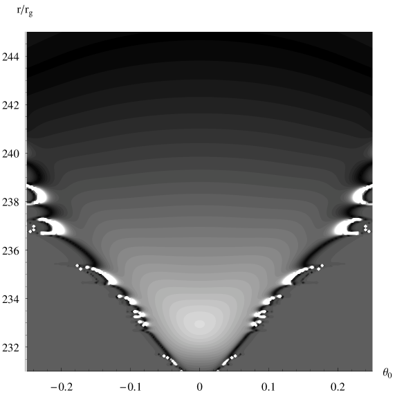
Figure 2. Temperature versus coordinates in the plane of variables $(r/r_{\rm g},\theta_{0})$ for the parameters $\Gamma=7/5$, $\varepsilon=0.03$, $c_{\infty}=0.00001$. The light area at the center has the highest temperature.

5. VALIDITY OF THE ASSUMPTIONS

To solve the problem, we made many assumptions. Let us substantiate them. For our estimates, we set $c_{\infty}=0.0002$.

(1) In most cases, the needed region is located far from the event horizon of the object, $r\gg r_{g}$, which allows us to consider the metric flat.

(2) The inclination of the streamline to the radial vector is near $r_{x}$. The solution for $n(r)$ yields $\Delta r=5\cdot 10^{5}\text{cm},r_{x}=10^{7}\text{cm},$ and $k_{x}=0.03$. The region is compressed almost uniformly for $\theta_{0}<0.3.$ whence, we can estimate $\alpha$ as $\alpha\approx\theta_{0}k_{x}r_{x}/\Delta r\approx 0.2$, and this is the maximum possible value for $\alpha$ within our range of parameters.

(3) To substantiate the possibility of ignoring the enthalpy of matter compared to the gravitational energy, we calculated the Mach number $M$. The ratio of the enthalpy to the kinetic energy for a non-relativistic gas is $2c_{s}^{2}/v^{2}(\Gamma-1)=2/M^{2}(\Gamma-1)$, reaching unity at $r_{x}$. However, this is true in a small region. This effect can be easily estimated by solving the equations for the effectively increased coefficient of the term responsible for the pressure. When the coefficients increases by a factor of $1.5$, $r_{x}$ decreases by approximately the same factor $1.5$, while $k_{x}$ increases by no more than $10\%$.

4. The smallness of ${\theta_{0}}^{25}k_{25}(r_{x})$ compared to $\theta_{0}k_{1}(r_{x})$ corresponds to $\theta_{0}<0.3$ at $r=r_{x}$,which corresponds to an area fraction of $0.036$ of the initial one at $r_{0}$. This implies that much $(>1/30)$ of the flow is subjected to strong compression. At a large radius, i.e., larger than $r_{x}$, each succeeding term $\theta^{2n+1}r_{2n+1}$ is much smaller than the preceding term, while this is not the case for $r<r_{x}$. This is most likely because the convergence is lost for $r<r_{x}$ in the method of solution used.

5. It is necessary to check as well that the results don’t depend on the $r_{0}$. Let us take $\varepsilon=0.58$ and $\Gamma=7/5$: when $r_{0}$ doubles, $k_{x}$ decreases by $10\%$ and $r_{x}$ decreases by $20\%$. The difference stems from the fact that the flow become slightly compressed, while moving from the sonic surface to $r_{0}$ , and, most importantly, its direction slightly changes. For smaller $\varepsilon$, the $r_{0}$ dependence of the parameters of the region is even weaker.

Note that the satisfactory accuracy of the results cannot be improved significantly by abandoning the assumptions made in favor of more accurate calculations. First, we used the first approximation for our calculations with a finite $\varepsilon$, and, second, we used its form at small radii where the firsts approximation grows compared to the zeroth solution. We cannot specify any initial conditions near the sonic surface, since the behavior of formula (5) is asymptotic for $r\rightarrow 0$.

To make progress in this field requires numerically solving an exact system of two nonlinear partial differential equations, one first-order equation and one second-order equation. In this case, we must reveal features that are many orders of magnitude smaller than the outer radius of integration or even the sonic surface, which can be achieved only by using adaptive methods with a variable step. In addition, we must numerically calculate the parameters of the separatrix surface (the boundary of the causally connected region) at which its smooth passage is realized, solve the time-dependent problem of establishment of this regime, show that it is stable, and find the percentage of cases, in which the accretion without shocks is possible. Such calculations are far beyond the scope of this paper.

6. PHYSICAL AND OBSERVATIONAL SIGNIFICANCE OF THE RESULT

Noteworthy among the features of the axisymmetric flow on a compact object observed so far is the tail convergence of streamlines behind a moving object during accretion in a region of cold dense dust, where star formation takes place.

The effect discussed in this paper has not yet been observed. The parameter $\Gamma=7/5$ has a very narrow validity range. For example, it is realized at the initial stage of accretion onto a compact object from dense clouds of molecular hydrogen before its dissociation (the equations with a constant $\Gamma$ cannot be used at all when the dissociation occurs).

Let us consider in more detail the accretion of a hot gas from H II regions with $\Gamma=5/3$ far from the massive object. The value of $\Gamma$ is the same on the sonic surface, since the gas density and temperature at infinity and on the sonic surface differ by a small factor (Bondi 1952). In this case, the angular momentum of the gas relative to the stellar center in a stable regime is very low. Although the electrons become relativistic and the adiabatic index decreases sharply $\Gamma=13/9$ starting from a certain distance (Shapiro and Teukolsky 1985), no region of anomalous compression is formed in this case.

Nevertheless, let us calculate the energy release in the region of streamline convergence for nonphysical constant values of $\Gamma<5/3$. The calculation will yield an upper limit for actual astrophysical objects. For our estimation, we assume that all of the observed radiation in the derived temperature range is only thermal bremsstrahlung (Shapiro 1973). Its intensity per unit volume is defined by the non-relativistic formula $\Lambda=cn^{2}T^{1/2}$ with the coefficient $c$ that depends weakly on the number density $n$ and temperature $T$. The intensity of the radiation for spherically symmetric accretion is then

$$L_{0}=\int\Lambda d^{3}r=\frac{8\pi}{3\Gamma-1}cn_{x}^{\Gamma+1}\left(\frac{r_{x}}{r_{g}}\right)^{3/2(\Gamma+1)}{r_{g}}^{3}.$$

The characteristic radial size of the region in our case is $\Delta r\approx r_{x}/5$, and the tangential size is $r_{\perp}\approx r_{x}\theta_{x}k_{x}$, where $\theta_{x}$ defines the maximum angle at radius $r_{0}$, starting from which flow lines contracts in $1/k_{x}$. The energy release $L_{x}$ in our region is

$$L_{x}\approx\Lambda_{x}\Delta r\pi r_{\perp}^{2}=Cn_{x}^{\Gamma+1}\pi\theta_{x}^{2}k_{x}^{-2\Gamma}r_{x}^{3}.$$

For our estimation, we set $\theta_{x}=0.5$. The ratio of the released energies can then be written as

$(14)$ $$\frac{L_{x}}{L_{0}}=\frac{3\Gamma-1}{160}k_{x}^{-2\Gamma}\left(\frac{r_{x}}{r_{g}}\right)^{3/2(1-\Gamma)}.$$

It follows from (14) and from the tables that the ratio of the released energies increases as the radius, at which the streamlines are focused, decreases. Let us calculate it for the minimum possible $\varepsilon$ when the focusing still takes place.We take the lower rows from the tables of parameters for the region of anomalous compression for $\Gamma=4/3$ and $\Gamma=7/5$. We find from (14) that $L_{x}/L_{0}$ reaches $100$; i.e., when the focusing is present, the Bondi-Hoyle accretion efficiency can increase up to a factor of $10^{2}$. For physically meaningful value $\Gamma=7/5$, the calculated ratio (14) actually specifies only an upper limit for $L_{x}/L_{0}$, since the gas dissociates rapidly and is subsequently ionized as it heats up, which ensures a transition to the regime with $\Gamma=5/3$ and is accompanied by a significant decrease in $L_{x}$. However, the proper allowance for the change in adiabatic index in the axisymmetric case is beyond the scope of this paper. Although the velocity dispersion of compact objects is much higher than the speed of sound in the surrounding cloud of gas and dust, the described regime with $\varepsilon<1$ can take place in certain cases at a low relative velocity of the gas cloud and the compact object. Such a change in energy release and accretion spectrum must be taken into account when analyzing experimental data to estimate the parameters of the black hole itself moving in regions of gas compression and its surrounding medium.

7. Acknowledgements

I wish to thank Prof. V.S. Beskin, my scientific adviser, for fruitful discussions. This work was supported in part by the Russian Foundation for Basic Research (project no. 05-02-17700).

8. References

1. V. S . Beskin and Yu. N. Pidoprygora, Zh. Eksp. Teor. Fiz. 107, 1025 (1995) [JETP 80, 575 (1995)].

2. H. Bondi and F.Hoyle, Mon. Not. R. Astron. Soc. 104, 273 (1944).

3. H. Bondi, Mon. Not. R. Astron. Soc. 112, 195 (1952).

4. A. R. Garlick, Astron. Astrophys. 73, 171 (1979).

5. S. L. Shapiro, Astrophys. J. 180, 531 (1973).

6. S. L. Shapiro and S. A. Teukolsky, Black Holes,White Dwarfs, and Stars: the Physics of Compact Objects (Wiley, New York, 1983; Mir,Moscow, 1985).