The Opacity of Spiral Galaxy Disks III:
Automating the “Synthetic Field Method”

Abstract

The dust extinction in spiral disks can be estimated from the counts of background field galaxies, provided the deleterious effects of confusion introduced by structure in the image of the foreground spiral disk can be calibrated. González et al. (1998) developed a method for this calibration, the “Synthetic Field Method” (SFM), and applied this concept to a HST/WFPC2 image of NGC4536. The SFM estimates the total extinction through the disk without the necessity of assumptions about the distribution of absorbers or the disk light. The poor statistics, however, result in a large error in individual measurements. We report on improvements to and automation of the Synthetic Field Method which render it suitable for application to large archival datasets. To illustrate the strengths and weaknesses of this new method, the results on NGC 1365, a SBb, and NGC 4536, a SABbc, are presented. The extinction estimate for NGC1365 is $A_{I}=0.6_{-0.7}^{+0.6}$ at 0.45 $R_{25}$ and for NGC4536 it is $A_{I}=1.6_{-1.3}^{+1.0}$ at 0.75 $R_{25}$. The results for NGC4536 are compared with those of González et al. (1998). The automation is found to limit the maximum depth to which field galaxies can be found. Taking this into account, our results agree with those of González et al. (1998). We conclude that this method can only give an inaccurate measure of extinction for a field covering a small solid angle. An improved measurement of disk extinction can be done by averaging the results over a series of HST fields, thereby improving the statistics. This can be achieved with the automated method, trading some completeness limit for speed. The results from this set of fields are reported in a companion paper (Holwerda et al., 2005b).

1 Introduction

The question of how much the dust in spiral galaxies affects our perception of them became a controversial topic after Valentijn (1990) claimed that spiral disks were opaque. Valentijn based his conclusion on the apparent independence of disk surface brightness on inclination. Disney (1990) objected to this conclusion, claiming instead that galaxy disks are virtually transparent and that Valentijn’s results were due to a selection effect. Others joined the controversy and within a few years a conference was organized to address the question of how best to determine galaxy disk opacity and what results could be obtained (Davies and Burstein, 1995).

Notably, White and Keel (1992) proposed a method to determine the opacity of a foreground disk galaxy in the rare cases where it partially occults another large galaxy. This technique has been followed up extensively with ground-based optical and infrared imaging (Andredakis & van der Kruit(1992), ; Berlind et al., 1997; Domingue et al., 1999; White et al., 2000), spectroscopy (Domingue et al., 2000), and HST imaging (Keel and White, 2001a, b; Elmegreen et al., 2001). Their results indicated higher extinction in the arms and a radial decrease of extinction in the inter-arm regions. Also the highest dust extinction was found in the areas of high surface brightness. Their sample of $\sim$20 suitable pairs seems now to be exhausted. This method furthermore assumes symmetry for the light distribution of both galaxies, so that a method independent of the light distribution is needed to confirm these results.

Instead of a single large background galaxy, the general field of distant galaxies can be used as a background source. Hubble (1934) noted the apparent reduction in the surface density of background galaxies at lower Galactic latitudes. Burstein and Heiles (1982) published a map of Galactic extinction based on the galaxy counts by Shane and Wirtanen (1967). Studies of extinction in the Magellanic clouds based on field galaxy counts have been done regularly (Shapley, 1951; Wesselink, 1961; Hodge, 1974; MacGillivray, 1975; Gurwell and Hodge, 1990; Dutra et al., 2001). More recently, attempts have been made to use field galaxy counts in order to establish the opacity in specific regions of nearby foreground galaxies from ground based data (Zaritsky, 1994; Lequeux et al., 1995; Cuillandre et al., 2001). Occasionally, the presence of field glaxies in a spiral disk is presented as anecdotal evidence of galaxy transparency (Roennback & Shaver(1997), ; Jablonka et al., 1998). The results of these studies have suffered from the inability to distinguish real opacity from foreground confusion as the reason for the decrease in field galaxy numbers.

González et al. (1998) (Paper I) introduced a new approach to calibrate foreground confusion which they called the “Synthetic Field Method”. While this new method can provide the required calibration for specific foreground galaxies, it is labor intensive and therefore ill-suited for the study of larger samples of galaxies of various types. In this paper we present the first results from a project to automate major steps in the Synthetic Field Method. After first providing a brief summary of the major features of the method, we describe how it was automated and which improvements we have made. As an illustration we have applied the new automated method to two galaxies, NGC 4536 and NGC 1365, and compared the results of our improved algorithms to those obtained on the former galaxy by González et al. (1998). In a companion paper (Holwerda et al., 2005b) we report on our application of the method to a data set consisting of 32 HST/WFPC2 pointings on 29 nearby galaxies.

2 The Synthetic Field Method

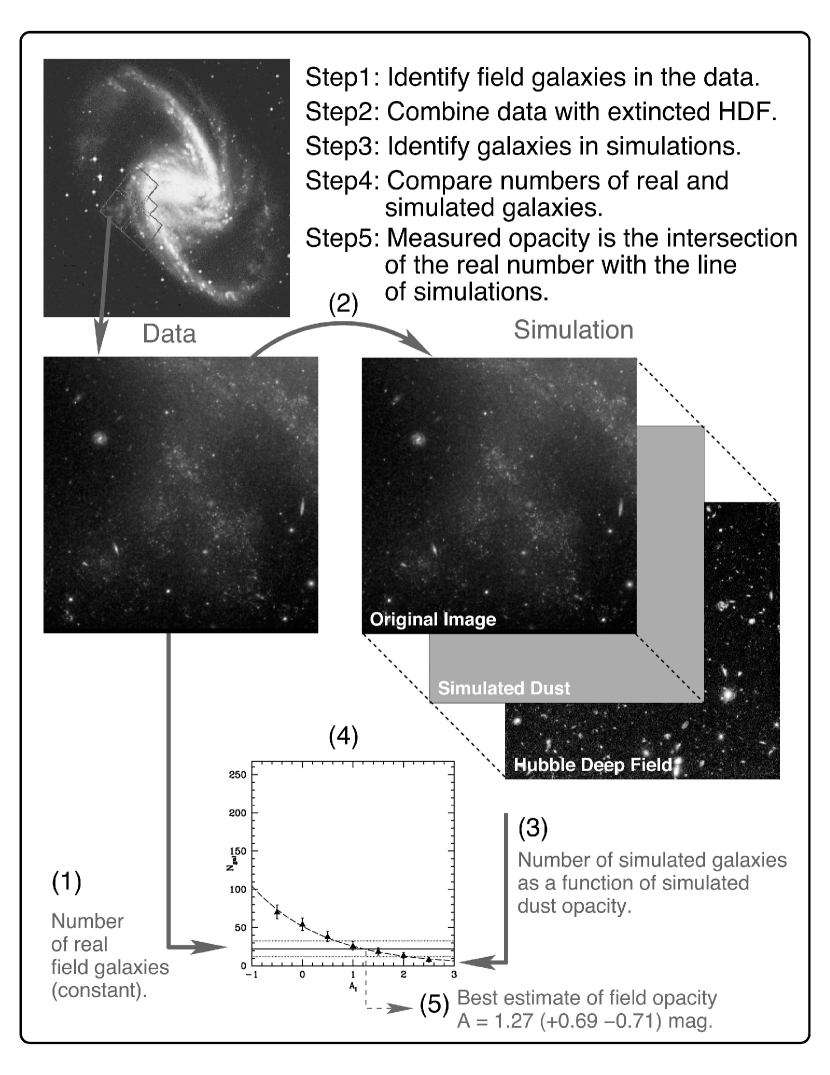
Figure 1: A schematic of the Synthetic Field Method (SFM). First, field galaxies are identified in the science field by a combination of automatic and visual selection. Secondly, a a HDF field is added to the science field in a series of simulations with different opacities. Field galaxies are selected from these simulated fields. Eq. 3 is fitted to these and uncertainties are estimated. Finally, the intersection between that relation and the number of galaxies gives the opacity of the area under consideration. In this case, the WF3 chip of NGC1365 has an average extinction of $1.3^{0.7}_{-0.7}$ magnitude.

Figure 1 shows a schematic of how the Synthetic Field Method is applied. Deep exposures of a nearby galaxy are obtained with the Wide Field Planetary Camera 2 (WFPC2) on the Hubble Space Telescope and background field galaxies are identified. Synthetic fields are then created by adding exposures from the Hubble Deep Fields (Williams et al., 1996, 2000) and the background field galaxy counts are repeated. The ratio of the surface density of real field galaxies to that of the HDF galaxies for any given region is a measure of the opacity in that region of the foreground galaxy. In practice, a series of synthetic fields is created with successively larger extinctions applied to the HDF galaxies until a match is obtained with the real field galaxy count, thus providing a quantitative measure of opacity in the foreground system. The method provides a way of calibrating the deleterious effects of confusion caused by the granular structure of dust, stars and luminous gas in the foreground galaxy. These effects are dramatic; for example a typical single WFPC2 chip (1$\farcm$2 $\times$ 1$\farcm$2) in the HDF may contain some 120 easily-identified background galaxies. This can drop to only 20 or 30 HDF galaxies when the foreground galaxy is present, and this number becomes even smaller for the larger values of a simulated foreground opacity. Counting background galaxies is therefore a battle against small number statistics, and reliable results are difficult to obtain on a single foreground galaxy. However, the method can in principle be applied to many nearby galaxies, and average opacities obtained e.g. as a function of radius for a sample of galaxies of similar morphological type.

2.1 Limits of the Synthetic Field Method

González et al. (2003) (Paper II) have discussed the broad limitations of the method in terms of the optimum distance interval for which it can be used most effectively given current and future ground and space-based imaging instruments. Two effects compete to limit the distance to which the SFM can be applied: First, if the foreground galaxy is too close, confusion from the “granularity” in the images, caused by a more resolved foreground disk, further reduces the number of bona fide field galaxies. Second, if the foreground galaxy is too distant, the small area of sky covered also reduces the numbers of field galaxies that can be used. These two effects conspire such that the optimum distance range for the Synthetic Field Method with HST/WFPC2 observations is approximately between 5 and 25 Mpc. Within this range there are of course many hundreds of galaxies visible to HST. However, now we are hindered by another limitation of the specific implementation of the Synthetic Field Method used by González et al. (1998), namely, that the identification of background and synthetic galaxies was carried out entirely visually, a time-consuming and laborious process. Clearly if any real progress is to be made, the process of identifying the field galaxies has to be automated (Holwerda et al., 2001, 2002a). Automated field galaxy identification has the benefits of speed and consistency across the datasets. Conversely in paragraph 5.1 we shall illustrate how it imposes a brightness limit on the selected objects.

3 Automation of the method

We have automated three steps in the Synthetic Field Method: first, the processing of archived exposures to produce combined images; second, the construction of catalogs of objects of simulated and science fields; and finally, the automatic selection of candidates for field galaxies, based on the parameters in the catalogs. A visual control on the process was retained by reviewing the final list of candidate field galaxies in the science field. We will now describe each step in the entire process in more detail.

3.1 Processing archival WFPC2 data

When data sets are recovered from the HST archive, the most recent corrections for hot pixels, bad columns, geometric distortions and the relative Wide Field (WF) and the Planetary Camera (Pc) CCD positions for the observation date are applied in the archive’s pipeline reduction. This pipeline system provides the user with a science data file and a quality file with positions of the bad pixels (Swam and Swade, 1999).

In order to stack multiple exposures, corrected for small position shifts and with the cosmic rays removed, we used the ’drizzle’-method (Mutchler and Fruchter, 1997), packaged in routines under IRAF/pyraf, with an output pixel scale of 0.5 of the original pixel and PIXFRAC between 0.8 and 1.0, depending on the number of shifts in the retrieved data. The PIXFRAC parameter sets the amount by which the input pixel is shrunk before it is mapped onto the output plane; a PIXFRAC lower then unity improves the sampling of the stacked image.

We developed a custom script to combine all exposures using python with the pyraf package (Greenfield and White, 2000), based on examples in the Dither Handbook (Koekemoer, 2002). The images are prepared for crosscorrelation in order to find the relative shifts; the background was subtracted (sky) and all none-object-pixels were set to zero (precor). Subsequently crosscorrelation images between exposures were made for each of the four CCDs (crosscor). The fitted shifts from these were averaged (shiftfind, avshift). Any rotation of an exposure was calculated from the header information and ultimately derived from the spacecraft orientation provided by the guide stars. All original exposures were shifted to the reference coordinates and a median image was constructed from these (imcombine). The median image was then copied back to the original coordinates (blot). The cosmic rays in each exposure were identified from the difference between the shifted median image and the original exposure (driz_cr). A mask with the positions of the cosmic rays and hot pixels, identified in the data quality file, was made for each exposure.

The exposures were drizzled onto new images and separately onto a mosaic with cosmic rays and bad pixels masked off (drizzle,loop_gprep). The new pixel-scale is fixed at 0$\farcs$05 but, to check the choice of PIXFRAC value, the script computed the rms of the weight image output from drizzle. The rms standard deviation should be between 15 and 30% of the mean.

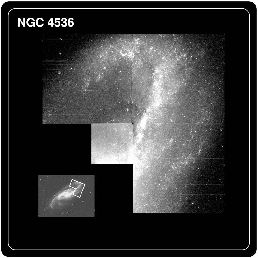
Figure 2: The mosaic made of the HST/WFPC2 exposure of the NE arm of NGC 4536, the inset is the Digital Sky Survey image with the WFPC2 footprint. Because of the lack of a dither greater then one pixel between epochs, some of the effects of masked bad columns can still be seen.

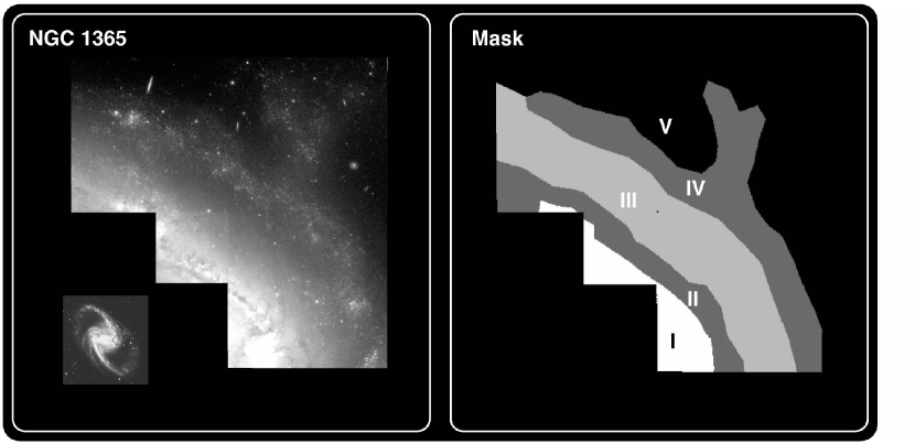
Figure 8: The mask used to denote crowded (I), arm (II, IV), inter-arm (III) and outside (V) regions in NGC 1365. Galaxy number counts are given for the inner arm region (II), inter-arm region (III), the “spur” (IV), and the outside region (V) in Figure 9.

For both galaxies used as examples here, there are many exposures made over several epochs. However the shifts for NGC 4536 are smaller than one original pixel (0$\farcs$1), and the bad columns of the CCD detector are unfortunately not covered by good pixels from other exposures (see Figure 2). Several exposures for NGC 1365 display shifts greater then a pixel, which helps to cover the bad columns and results in a cleaner looking image (Figure 8). In both cases the number of shifts was sufficient for a PIXFRAC of 0.8 with the new pixel scale of 0$\farcs$05.

3.2 Making object catalogs

A modified version of Source Extractor v2.2.2 (hereafter SE, Bertin and Arnouts (1996)) was used to generate catalogs of objects for the science fields and simulations. The F814W (“I”-band) fields were used for detection. Catalogs for the F555W (“V”-band) fields were constructed using the dual mode; the photometry was done on the V field using the I apertures. All the structural parameters were derived from the I images. In Table 1 we list our choice of SE input settings. Table 2 lists the intrinsic output parameters from SE and Table 3 the new output parameters we added. In addition the position of objects on the CCD and on the sky are in the catalogs.

It was already noted by Bertin and Arnouts (1996) that the success of SE’s native star/galaxy classification parameter was limited to the very brightest objects. Several other parameters are described in the literature for the classification of field galaxies. Abraham et al. (1994) and Abraham et al. (1997) used asymmetry, contrast and concentration to identify Hubble type of galaxies. Similarly Conselice (1997, 1999); Conselice et al. (2000); Bershady et al. (2000); Conselice (2003) used asymmetry, concentration and clumpiness as classifiers. By adding some of these parameters or our approximations of them to the Source Extractor code, we obtained a better parameter space within which to separate field galaxies from objects in the foreground galaxy.

3.3 Selection of field galaxy candidates using “fuzzy boundaries”

The characteristics as determined by SE for field galaxies and foreground objects are very similar; for example, we show in Figure 3 the distribution of the FWHM of all objects and that of the HDF galaxies. This similarity exists because there are many extended foreground objects: star clusters, HII regions, artifacts from dust lanes, diffraction spikes near bright stars and “objects” which are blends of several objects. The field galaxies also span a range in characteristics, as can be seen in the Hubble Deep Fields. Simple cuts in parameter space can do away with some objects that are clearly not field galaxies, but the field galaxies cannot be uniquely selected that way.

In order to select objects most likely to be field galaxies, we developed a “fuzzy boundary” selection method. From a training set of objects with known field galaxies, the fraction of field galaxies in a bin of a relevant SE output parameter can be determined. Our training set consists of catalogs of the simulations with no artificial extinction of five galaxies in our sample (NGC 1365, NGC 2541, NGC 3198, NGC 3351 and NGC 7331). In these catalogs, the added HDF galaxies were identified by their positions . The fraction of HDF galaxies in a SE parameter bin can then be used as a probability that an unknown object with a value in that bin is a field galaxy. By multiplying these fractions of HDF galaxies for every relevant SE parameter ($P_{i}$) for each object, an overall galaxy-likeness score (P) for that object is obtained:

$$P=\left({\prod P_{i}\over(\prod P_{i})+(\prod(1-P_{i}))}\right)$$ (1)

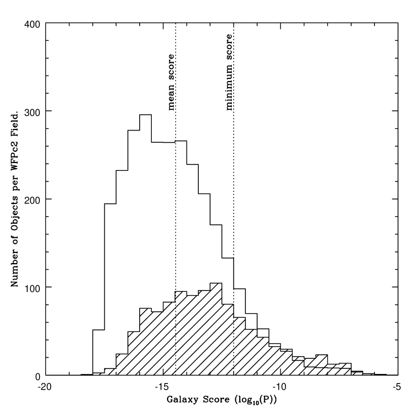
Figure 4: The distribution of galaxy score for objects in our science fields. $P=\left({\prod P_{i}\over(\prod P_{i})+(\prod(1-P_{i}))}\right)$. The shaded area is the average histogram for HDF galaxies (both North and South). Objects to the right are more galaxy-like. The majority of field galaxies is indistinguishable in properties from the objects in the foreground galaxy. Only the higher scoring tail (about -12 and above) can be used for the opacity measurement. The mean score of all objects is indicated, together with the minimum score for selection.

We used the distribution of the log of these probabilities ($log_{10}(P)$) as a sliding scale of the galaxy-like quality of an object. The distribution of $log_{10}(P)$ for objects in 21 science fields is plotted in Figure 4, with the distribution of HDF-N/S objects scaled for comparison. The advantage of using an overall scale is that an object can fare poorly for one SE parameter but still make the selection. This makes the boundaries for any single parameter in parameter space of the field galaxies “fuzzy” . All the structural parameters marked in Tables 2 and 3 as well as the V-I color from the smallest aperture were used in computing the galaxy score. The selection criterion is an overall score ($log_{10}(P)$) greater than the $log_{10}$ of the mean score of all objects plus 2.5, that is:

$$log_{10}(P)>log_{10}(P_{mean})+2.5$$ (2)

Field galaxies missed by this procedure are not selected in either simulation or real data and therefore do not influence our comparison. There are however, still some contaminant foreground objects that are selected as well and these have to be identified and discarded by visual inspection.

3.4 Visual identification of contaminants

A human observer can pick out contaminants based on contextual information not contained in the SE parameters. There are five broad categories of remaining contaminants: star-clusters, diffraction spikes, HII regions, artifacts from dust lanes, and blended objects.

Stellar clusters, both young open clusters and globular clusters, are associated with the foreground galaxy. At the distance of the Virgo cluster, these are often of approximately the size and color of more distant E0 field galaxies. Young open clusters are often found in spiral arms and are very blue, while globular clusters can be identified by the slightly different brightness profile. Bright stars in our own galaxy result in false selections. Their wings are extended, often blending with other objects, and the diffraction spikes resemble edge-on galaxies. The proximity of these false selections to the bright star makes them easily visually identifiable. HII regions resemble blue irregular galaxies but are invariably found in the proximity of several blue open clusters. Dust lanes superimposed on a smooth disk may result in an extended ‘object’, which is often reddened. This results in severe contamination, especially in flocculant spiral galaxies, making their inner regions unsuitable for the SFM.

Blended objects are by far the largest source of contamination. A blend of one of the above objects with a small clump of stars is likely to be selected as a candidate field galaxy. Also in a nearby foreground galaxy, the granularity of the partly resolved disk may result in contamination from blended clumps of disk stars. SE does a deblending of peaks in the flux, but the choice of parameters governing this is a trade-off between deblending objects and keeping extended objects intact. The candidate objects from the science fields were marked in the F814W image for visual inspection together with their score and color. Objects deemed to be contaminants were removed. All the candidates from the science fields are removed from the synthetic field candidate list.

However, the numbers of simulated galaxies have to be corrected for any false selections as a result of a blend of a faint HDF object and a foreground one. To correct the numbers from the simulated fields, the same visual check was done on the simulations from both galaxies with no artificial extinction (A=0) and in the case of NGC1365 also in an extincted simulation (A=2). The candidate objects were in this case the real galaxies, the simulated galaxies and the misidentifications, both from the original field and as a result from the addition of the HDF objects. The percentage of HDF objects rejected, mostly blends, in these visual checks are given in Table 5 per typical region, an indicator of the measure of crowding. These percentages do not seem to change much as a function of either choice of galaxy or simulation. To correct for blends of HDF and foreground objects, a fixed percentage of the remaining simulated galaxies from a typical region is removed after the removal of the science field’s candidates. These adopted percentages are also given in Table 5 for each typical region.

4 Improvements in the “Synthetic Field Method”

In the process of automating the SFM we have introduced several improvements. First, exposures were combined with the “drizzle” routine, improving the sampling of the final image. Second, we have provided for a less observer dependent selection of field galaxies. These two categories of improvements we have described in the previous sections. Third, extra simulations were made, biases and uncertainties were estimated, and opacities were obtained based on segments of the images with similar characteristics. We will describe these improvements in this section.

4.1 Foreground galaxy segmention

The SFM provides an average opacity for a certain region of the foreground galaxy. González et al. (1998) reported opacities for regions defined by WFPC2 chip boundaries. Ideally, an average opacity is determined for a region of the foreground galaxy that is homogeneous in certain characteristics: arm or inter-arm regions, deprojected radius from the center of the galaxy, or a region with the same surface brightness in a typical band.

In our treatment, the mosaiced WFPC2 fields are visually devided into crowded, arm, inter-arm and outside regions. This step is applied to the catalogs of objects by tagging each object according to its general location in the foreground galaxy. Objects from the crowded regions were ignored in the further analysis. The deprojected radial distance for each object was also computed from the inclination, position angle and position of the galaxy center taken from the 2MASS Large Galaxy Atlas (Jarrett et al., 2003) or, alternatively, the extended source catalog (Jarrett et al., 2000); the distance was taken from Freedman et al. (2001). The surface brightness based on the HST/WFPC2 mosaics or a 2MASS image could also be used to define a partition of the WFPC2 mosaics.

4.2 Simulated fields

Simulated fields are made by taking one WF chip from either the northern or southern Hubble Deep Field (HDF-N or HFD-S), extincting it with a uniform grey screen, and adding it to a data WF chip. This results in six separate simulations for each opacity and data chip: one for each HDF-N/S WF chip. Simulations for seven opacity levels were made, ranging from -0.5 to 2.5 magnitudes of extinction with steps of 0.5 magnitude. The negative -0.5 opacity simulation was added to obtain a more accurate fix on the point of zero opacity. The use of a grey screen in the simulations was chosen because its effect on the numbers of field galaxies is similar to that of a distribution of dark, opaque clouds with a specific filling factor and size distribution.

To infer the opacity ($A_{I}$) from the numbers of field galaxies ($N$), González et al. (1998) use:

$$A_{I}=-2.5~{}C~{}log\left(N\over N_{0}\right)$$ (3)

$N_{0}$ is the normalisation and C the slope of the relation between the number of field galaxies and the extinction. They depend on the crowding in the field and total solid angle. Crowding limits the number of field galaxies. When it dominates the loss of field galaxies, the relation becomes much flatter ($C>>1$). González et al. (1998) found C to differ with the extinction law used in the simulations in the same foreground field. We use grey extinction but vary the foreground field.

For each field, we fit the relation between $A_{I}$ and $log(N)$, minimising $\chi^{2}$ to the average numbers of field galaxies found in the simulated fields with known extinctions . The intersection of this curve with the real number of field galaxies yields an average opacity estimate for the region. See Figures 6, 9, 10 and 11 for the fitted relation (dashed line) and the number of field galaxies from the science field (solid line).

4.3 Field galaxy numbers: uncertainties and systematics

There are four quantities which affect the numbers of field galaxies besides dust absorption. They are: crowding, confusion, counting error and clustering. Crowding and confusion introduce biases which need to be calibrated. Counting and clustering introduce uncertainties in the galaxy numbers that must be estimated. In addition, the clustering could possibly introduce a bias if the reference field is not representative for the average.
Crowding effectively renders the parts of the image of little use for the SFM. Typically these are stellar clumps, the middle of spiral arms and the center of the foreground galaxy. The strongly crowded regions in the WFPC2 mosaics were masked off and not used in further analysis.
Confusion is the misidentification of objects by either the selection algorithm or the observer. Misidentification by the algorithm is corrected for by the visual check of the science fields (detailed in section 3.4). In order to correct the numbers of simulated objects, the candidates from the science field, including the misidentifications, are removed and subsequently the average rejection rate from Table 5 is applied to the remaining objects from each typical region. The typical regions are a measure for the crowding, the main source of the remaining confusion due to blends of HDF and foreground objects.
Counting introduces a Poisson error. If the numbers are small ($N<100$), $\sqrt{N}$ underestimates the error and the expressions by Gehrels (1986) for upper and lower limits are more accurate. We adopted these for both simulated and real galaxy numbers using the expressions for upper and lower limits for 1 standard deviation.
Clustering introduces an additional uncertainty in the number of real galaxies in the science fields, as the background field of galaxies behind the foreground galaxy is only statistically known. This variance in the background field necessitates a prudent choice of reference field for the background in the simulated fields as otherwise an inadvertent bias in the opacity measurement can be introduced (see also section 4.3.1).

The standard deviation of this uncertainty can be estimated using a similar argument to the one in Peebles (1980) (p.152), replacing volume by solid angle and the three dimensional 2-point correlation function by the two dimensional one ($\omega(\theta)$). The resulting clustering uncertainty depends on the depth of the observation and the solid angle under consideration.

$$\sigma^{2}_{clustering}=N+N^{2}\times\left(A(m_{lim},Filt){2\Gamma(2+\delta\over\Gamma(2+{\delta\over 2})\Gamma(3+{\delta\over 2})}\theta_{max}^{\delta}\right)$$ (4)

where $A(m_{lim},Filt)$ is the amplitude, depending on photometric band and brightness interval and $\delta$ is the slope of the 2-point correlation function $\omega(\theta)=A~{}\theta^{\delta}$. N is the number of field galaxies and $\theta_{max}$ characterises the size of the solid angle under consideration. The slope, $\delta$ is usally taken to be -0.8 and the value of term between $A(m_{lim},Filt)$ and $\theta_{max}^{\delta}$ in equation 4 becomes 1.44. The $A(m_{lim},Filt)$ values from Cabanac et al. (2000) are used to compute $\omega(\theta)$ and the resulting clustering uncertainty as they are for the same filters (V and I) and integrated over practical brightness intervals with a series of limiting depths . González et al. (1998) claim a completeness of galaxy counts up to 24 mag for one of their fields. We estimate the limiting magnitude by the value above which 90% of the simulated galaxies with no dimming (A=0) lie. We extrapolated the relation between limiting magnitude and amplitude ($A(m_{lim},Filt)$) from Cabanac et al. (2000) to model the clustering error to higher limiting magnitudes. For each field we characterise the limiting depth by the interval in which the majority of simulated field galaxies lie in the simulations with no opacity. Alternatively we could have used a very large number of background fields in the simulations and determined the possible spread in field galaxy numbers due to clustering from those. For practical reasons we used the average of simulations with the HDF-N/S fields and estimated the uncertainty in the real number of field galaxies from equation 4. The uncertainties in opacity owing to the clustering uncertainty in the original background field are given separately in Table 6, and in Figures 6, 9, 10 and 11.

The clustering error and Gehrels’s counting uncertainties were added in quadrature to arrive at the upper and lower limits of uncertainty for the real galaxies. Simulated counts only have a counting uncertainty as these are from a known typical background field.

From the errors in the number of field galaxies in each simulation and in the real number of field galaxies, the uncertainty in the average opacity A can then be derived from equation 3. A single field gives a highly uncertain average value for extinction. Averaging over several galaxies will improve statistics and mitigate the error from field galaxy clustering.

4.3.1 The HDF as a reference field

The SFM uses the Hubble Deep Fields as backgrounds in the synthetic fields. The counts from these are taken to be indicative of the average counts expected from a random piece of sky, suffering from the same crowding issues as the original field. In this use of the HDF-N/S as the reference field, the implicit assumption is that it is representative of the average of the sky. If they are not, the difference in source counts between the HDFs and the average sky introduces a bias in the synthetic fields and hence a bias in the resulting opacity measure.

The position of the HDF North was selected to be unremarkable in source counts and away from known nearby clusters (Williams et al., 1996). The position of the HDF South was dictated by the need to center the STIS spectrograph on a QSO but Williams et al. (2000) assert that the source count in HDF-S was unlikely to be affected by that. In addition Casertano et al. (2000) point out that the HDF-S was chosen such that it was similar in characteristics to HDF-N. The selection strategy of the Deep Fields therefore does not seem to be slanted towards an overdensity of sources.

To test the degree to which the Hubble Deep Fields are representations of the average field of sky, the numbers of galaxies we find can be compared to numbers from the Medium Deep Survey (Griffiths et al., 1994), a program of parallel observations with the WFPC2, also in F814W. Several authors (Casertano et al., 1995; Driver et al., 1995a, b; Glazebrook et al., 1995; Abraham et al., 1996; Roche et al., 1997) report numbers of galaxies as a function of brightness in these fields. Casertano et al. (1995); Driver et al. (1995a); Glazebrook et al. (1995); Abraham et al. (1996); Roche et al. (1997) present averages for multiple fields and Driver et al. (1995b); Abraham et al. (1996) the numbers from deep fields, the latter for the HDF-N. In Figure 5, we plot these numbers of galaxies as a function of magnitude. Also the number of sources identified by our algorithm as field galaxies in the Hubble Deep Fields are also plotted. The average of the Hubble Deep Fields (filled circles) corresponds well to the curves from the literature up to our practical limiting depth of 24 mag. The difference between the north and south HDF never exceeds the Poisson uncertainty of the average, and even changes sign for galaxies fainter then 24 mag.

From Figure 5, we conclude that the average of the Hubble Deep Fields is a good representation of the average field in the sky, and the numbers of galaxies from the simulations do not need to be corrected for any bias resulting from an atypical reference field. In any case, any residual bias would be trivial compared to the uncertainties in individual WFPC2 fields, but could have become important when combining counts from many fields as we have done in our companion paper (Holwerda et al., 2005b).

4.4 Inclination correction

Any inclination correction of the opacity values depends on the assumed dust geometry. A uniform dust screen in the disk would result in a factor of cos(i) to be applied to the opacity $A_{I}$. However if the loss of field galaxies is due to a patchy distribution of opaque dust clouds, the correction becomes dependent on the filling factor, cloud size distribution and cloud oblateness. All the extinction estimates ($A_{I}$) and the values corrected for inclination ($A_{I}\ \times\ cos(i)$) are listed in Table 6, assuming a simple uniform dust screen.

5 Examples: NGC 4536 and NGC 1365

NGC 4536 (González et al., 1998) was reanalyzed as a test case to provide a comparison between observers and versions of the SFM. NGC 1365 was one of the first galaxies analyzed with the improved method (Holwerda et al., 2002b) and provides a good example of how the method works for an image which can be segmented into different regions. See Table 4 for basic data on both galaxies and the observations which made up the data set.

5.1 NGC 4536, comparing observers

Identifying field galaxies remains a subjective process, and different software systems as well as different observers will differ in their identifications. However, as long as the same selection criteria are applied to simulations and science objects , a good estimate of dust extinction can be made. Figure 6 shows the extinction measurements from González et al. (1998) and this paper.

The numbers of field galaxies and subsequent derived opacities in the combined WF2 and 3 chips are very similar for González et al. (1998) and this paper. The results for WF4 seem to differ however, both in numbers of field galaxies found as the derived extinction. WF4 was analysed separately by González et al. (1998) as it was less crowded than the other two WFPC2 chips, so field galaxies could be found to a higher limiting depth. González et al. (1998) estimate the limiting magnitude for the WF4 chip as 24 magnitude and for the WF2&3 field as 23 mag. The selection of objects as candidate field galaxies by our algorithm however imposes a limiting depth to which objects are selected ( $I\approx 23mag$). This effect can be seen in the cumulative histogram of real galaxies (Figure 7), especially in the WF4 where the numbers from González et al. (1998) are still increasing beyond 24 magnitude. The effect is less pronounced in the simulated numbers (Figure 7 bottom right). These differences in numbers at the faint end are the cause for the difference in derived opacities for González et al. (1998) and this paper. However a lower limiting magnitude makes the derived extinction less accurate (lower number statistics and a bigger uncertainty due to clustering), not inconsistent with each other.

If the numbers from González et al. (1998) are limited to the same limiting magnitude as ours, the numbers from science and simulated fields galaxies match up. In addition, in a visual check, both observers agree on the identification of these brighter field galaxies. Given this, we feel that the automated method’s trade of depth for speed is warranted.

By automatically selecting objects and correcting the simulations for the pruning of galaxies in the visual step, we are confident that we select similar sets of field galaxies, to the same limiting depth, with a high degree of certainty in both simulated and real fields.

5.2 NGC 1365: arm and inter-arm extinction

González et al. (1998) remarked on the importance of distinguishing between arm regions, regions between the arms (inter-arm), and outside regions. Beckman et al. (1996), White et al. (2000) and Domingue et al. (2000) all found that extinction was more concentrated in the spiral arms. NGC 1365 provides a nice example of an arm with a crowded region, an inter-arm region, a spur, and some outside area (see Figure 8). The opacity measurements of these regions are plotted in Figure 9. The “spur” region (IV), the inter-arm region (III) and the region outside (V) show some opacity but all are still consistent with none. Most of the extinction in this galaxy is in the main inner arm (II): $A=3.9_{-3.5}^{+2.6}$. For such a small subdivision in only one field, this opacity measure is very uncertain. However, by combining measurement in several arm regions in several galaxies, as we have done in Holwerda et al. (2005b), we are confident that a reliable and meaningful estimate can eventually be made.

5.3 NGC 4536 and NGC 1365: Radial profile of extinction

One of the new applications of the SFM introduced here is to compare the numbers of field galaxies in an annular region of the mosaic between two deprojected radii. Figures 10 and 11 show results for four sets of annuli for NGC 4536 and NGC 1365, respectively. We present the radial opacity values found in this way in Figure 12 for both NGC 4536 and NGC 1365. Noticeable is the occurrence of comparatively high values of opacity at different radii. This depends on whether or not the area in the radial annulus is dominated by arm regions or inter-arm type regions.

The NGC1365 profile shows a steep rise in the inner region and the peak in the NGC 4536 profile corresponds to the prominent arm there. Individual errors in these measurements remain quite large due to the poor statistics and the clustering uncertainty in the field of galaxies.

Comparing these values to those in Figure 12 of White et al. (2000), the peak values in these radial plots, at 0.3 and 0.75$R_{25}$ respectively (see Figure 12), are completely consistent with the arm extinction values found by those authors. When combining the radial profiles of our entire sample of HST fields, we should keep in mind the importance of spiral arms in the radial extinction profile.

5.4 Surface Brightness

Giovanelli et al. (1995); Tully et al. (1998); Masters et al. (2003) found that disk extinction correlates with total galaxy luminosity. With the SFM we can have a more detailed look at the correlation between the light in a galaxy and the extinction. The higher extinction found in spiral arms is an indication that this correlation is also present in our data. However, with few points obtained from only two fields, no relation can be reliably detected. A plot of the extinctons and surface brightnesses derived from all our fields will be presented in a future paper.

6 Conclusions

We have shown that the Synthetic Field Method as developed by González et al. (1998) can be successfully automated and applied to a large variety of fields. As most classification schemes break down in crowded regions, some visual check by a human observer will remain necessary, either to deem the region too crowded or to check the classification of the objects. The bias thus introduced is also calibrated using synthetic fields. The great increase in throughput provided by the automation opens up the possibility to infer dust absorption in a wide range of fields available in the HST archive.

In the process of automating the SFM, we introduced some improvements. The quality of the images has been improved with the drizzle technique. The selection of field galaxies is less observer-dependent and much faster. Extra HDF-S control fields were added to mimic the average background field. The results are now given per typical region instead of per chip. Improved estimates of the uncertainties due to the random error and the clustering of the field galaxies have also been incorporated.

Future improvements of this technique could include the use of multi-color imaging or field spectroscopy in order to more unambiguously identify the field galaxies. An improved object classification, based on different data and with a more sophisticated algorithm, could in the future make the need for a visual check of objects redundant.

The apparent difference between derived extinctions between this paper and González et al. (1998) for NGC4536 can be accounted for by a difference in limiting depth and the uncertainty it brings with it. However the agreement between observers in their identifications of the brighter objects suggest a consistency of the method across identification schemes.

The radial dependencies of opacity in our examples show evidence of substantial extinction, $A_{I}=0.6_{-0.7}^{+0.6}$ mag for NGC 1365 at half the $R_{25}$ and $A_{I}=1.6_{-1.3}^{+1.0}$ at 0.75 $R_{25}$ radii for NGC 4536. These extinction values at these radii are consistent with those reported by White et al. (2000). Most of this extinction seems to concentrate in the arm regions of these galaxies.

While the SFM itself is independent of assumptions about the dust geometry in the foreground galaxy, the inclination correction for the opacity is not. Corrections based on a simple screen have been presented, a more thorough discussion of other possibilities is considered in the companion paper (Holwerda et al., 2005b).

The principal advantage of this method is that no assumption about the distribution of either absorbers or the underlying starlight goes into the measurement. However, the small number statistics in individual regions result in large uncertainties for single measurements. Averages over several fields will improve this by increasing the statistics and averaging out the field galaxy clustering. The application of this method to a substantial set of archival HST/WFPC2 images is presented in Holwerda et al. (2005b)

7 Acknowledgements

We would like to thank A. Koekemoer for his help with the “drizzle” method, E. de Vries and I. Smail for help with modifying the Source Extractor code, and H. Ferguson and S. Casertano for insightful discussions on the Synthetic Field Method. Earlier versions of this manuscript were read by E. Brogt.

This research has made use of the NASA/IPAC Extragalactic Database (NED) which is operated by the JPL, CalTech, under contract with NASA.

This work is primarily based on observations made with the NASA/ESA Hubble Space Telescope and obtained from the data archive at the Space Telescope Institute. Support for this work was provided by NASA through grant number HST-AR-08360 from the Space Telescope Science Institute (STScI). STScI is operated by the association of Universities for Research in Astronomy, Inc. under the NASA contract NAS 5-26555. We are also grateful for the financial support of the STScI Director’s Discretionary Fund (grant numbers 82206 and 82304) and the Kapteyn Institute of Groningen University

Figure 3: The distribution of the FWHM (in pixels), determined by Source Extractor, of all the objects in 21 of the science fields, averaged over the number of fields. The shaded area is the histogram per WFPC2 field for HDF galaxies (both North and South). A selection limit based on this parameter only would not have done nearly as well as our scoring system.

Figure 5: The numbers of field galaxies per magnitude per square arcminute from several authors. All counts were in the I band (F814W). The HDF points are the average of all our counts for HDF-N and HDS-S. Triangles and squares are our averages for HDF-N and HDF-S respectively. The numbers by Casertano et al. (1995) are from pre-refurbished WFPC data, accounting for the slightly higher numbers. The numbers found by Abraham et al. (1996) for the HDF-N are slightly higher then ours for the fainter objects as our selection started to discard some. The dashed lines are from single deep WFPC2 exposures (Driver et al., 1995b; Abraham et al., 1996), the solid lines from multiple exposures (Casertano et al., 1995; Glazebrook et al., 1995; Driver et al., 1995a; Abraham et al., 1996; Roche et al., 1997).

Figure 6: The number of simulated galaxies per WF chip as a function of extinction for the González et al. (1998) result (left panels) and this paper (right panels). Top panels are the average for WF2 and 3, combined by González et al. (1998) due to similar appearance and poor statistics. The bottom panels are WF4. The errorbars for the simulated numbers (filled triangles) are Poisson uncertainties only. The dashed line is the best fit ($A_{I}=-2.5\ C\ log_{10}(N/N_{0})$). The solid horizontal line is the real number of field galaxies found, the dotted horizontal lines mark the uncertainty in this number due to counting and clustering combined. The opacity measurement shows also the total error, and that part of the error which is due to clustering in brackets. The limiting magnitude $M_{lim}$ was determined from the A=0 simulation.

Figure 7: The cumulative histograms of number of field galaxies with their magnitude (MAG_ISO) for our identifications (solid lines) and González et al. (1998) (dotted lines) for wf2&3 (left panels) and wf4 (right), science field galaxies (top) and simulated field galaxies (bottom).

Figure 9: Simulated and real numbers of field galaxies in typical regions in NGC 1365; “arm” regions on either side of the inter-arm region (region II and IV in figure 7), the “inter-arm” region (region III) and the “outside” region (region V). Errorbars, notation and curves same as the right panels in Figure 6. C is the fit for equation 3. $M_{lim}$ is the limiting magnitude used to compute the clustering uncertainty.

Figure 10: The numbers of real field galaxies and those of simulated field galaxies plotted as a function of simulated opacity in areas of de-projected radius from the centre of NGC 4536. The radii are expressed in $R_{25}$, derived from the B-band photometric diameter ($D_{25}$) from the RC3 catalog (de Vaucouleurs et al., 1991). Errorbars, notation and curves same as the right panels in Figure 6. C is the fit for equation 3. $M_{lim}$ is the limiting magnitude used to compute the clustering uncertainty.

Figure 11: The numbers of real field galaxies and those of simulated field galaxies plotted as a function of simulated opacity in areas of deprojected radius from the center of NGC 1365. The radii are expressed in $R_{25}$, derived from the B-band photometric diameter ($D_{25}$) from the RC3 catalog (de Vaucouleurs et al., 1991). Errorbars, notation and curves same as the right panels in Figure 6. C is the fit for equation 3. $M_{lim}$ is the limiting magnitude used to compute the clustering uncertainty.

Figure 12: The dust extinction plotted as a function of radius, expressed in $R_{25}$. The opacity of NGC 1365 (top) for the entire field, with all radii combined, is $A=0.5_{-0.3}^{+0.3}$ and for NGC 4536 (bottom plot), the opacity of the entire field is, $A=0.9_{-0.4}^{+0.4}$.

Table 1: Source Extractor Input Parameters

Parameter	Value	Comments
PIXEL_SCALE	0.05	Scale in arcsec after drizzling
SEEING_FWHM	0.17	FWHM of the HST PSF
BACK_SIZE	32	Background estimation anulus.
BACK_FILTERSIZE	3	Background estimation smoothing factor.
BACKPHOTO_TYPE	LOCAL	Photometric background.
BACKPHOTO_THICK	32	Photometric background anulus.
DETECT_MINAREA	10	Minimum number of pixels in object.
FILTER	Y	Smooth before detection?
FILTER_NAME	gauss_4.0_7x7.conv	Smoothing kernel, gaussian with 4 pixel FWHM.
DEBLEND_NTHRESH	32	Number of deblending thresholds.
DEBLEND_MINCONT	0.001	Deblending minimum contrast.
CLEAN	Y	Remove bright object artifacts?
CLEAN_PARAM	1.5	Moffat profile $\beta$ used for cleaning.
PHOT_APERTURES	3,5,11,21,31	Fixed aperture diameters.
GAIN	7.0	Gain of the Wide Field CCD

Table 2: Source Extractor Intrinsic Output Parameters

Name	Description	Unit	Used	Comments
A_IMAGE	major axis	pixel	*
B_IMAGE	minor axis	pixel		a
ELLIPTICITY	1 - B_IMAGE/A_IMAGE	$\cdots$	*
FWHM_WORLD	FWHM assuming a gaussian core	deg	*
FLUX_RADIUS	Fraction-of-light radii	pixel	*	b
ISOAREA_IMAGE	Isophotal area above analysis threshold	pixel2	*
CLASS_STAR	S/G classifier output	$\cdots$	*	c
MAG_ISO	Isophotal magnitude	mag		d
MAG_AUTO	Kron-like elliptical aperture magnitude	mag
MU_MAX	Peak surface brightness above background	mag $/$ arcsec2	*	e
MAG_APER	Fixed aperture magnitude vector	mag	*	f

Table 3: Source Extractor Output Parameters we have added

Name	Description	Used	Unit	comments
CONCENTRATION	Abraham concentration parameter	*	$\cdots$	a
CONTRAST	Abraham contrast parameter	*	$\cdots$	b
SQR_ASYMMETRY	Point-asymmetry index (difference squared)		$\cdots$	c
ASYMMETRY	Point-asymmetry index (absolute difference)	*	$\cdots$	d
MAJOR_AXIS_ASYM	Major axis asymmetry index		$\cdots$	e
MINOR_AXIS_ASYM	Minor axis asymmetry index		$\cdots$	e
MOFFAT	Computed Moffat magnitude		mag	f
MOFFAT_RMS	Ratio RMS deviation to computed Moffat flux.		$\cdots$	f
MOFFAT_RES	Ratio absolute residue to computed Moffat flux.		$\cdots$	f

Table 4: HST Archive Data Examples

Galaxy	Type	Prop. ID.	Exp Time		Distance.	$R_{25}$	Inclination
			$V_{F555W}$	$I_{F814W}$	(Mpc.)	(Kpc.)	(Deg.)
					(1)	(2)	(3)
NGC 1365	SBb	5972	66560.0	16060.0	17.95	27.3	34
NGC 4536	SAB(rs)bc	5427	68000.0	20000.0	14.93	16.5	63

Table 5: Visual Rejection percentages

Galaxy	Total	Crowded	Arm	Inter-arm
NGC4536	22	89	50	16
NGC1365	35	100	56	19
NGC1365 (A=2)	55	97	66	31
adopted rates	-	100	50	20

Note. — Average rejection percentages of added HDF objects in visual checks identical to those in the real fields, using all the zero extinction simulations. We use rejection fractions for the average synthetic field counts of 0.5 and 0.2 for arm and inter-arm regions respectively to correct the simualted numbers for the visual step on the real number of field galaxies.

Table 6: Extinctions for different regions in the fields

Region	$A_{I}$	$\Delta A_{c}$	$A_{I}\times cos(i)$
	(1)	(2)
NGC1365
WFPC2	$0.5^{+0.3}_{-0.3}$	$(\pm 0.3)$	$0.4^{+0.3}_{-0.3}$
Arm(II)	$3.9^{+2.6}_{-3.5}$	$(\pm 1.8)$	$3.2^{+2.2}_{-2.9}$
Arm(IV)	$-0.7^{+1.1}_{-1.1}$	$(\pm 0.8)$	$-0.6^{+0.9}_{-0.9}$
Interarm(III)	$0.4^{+0.6}_{-0.6}$	$(\pm 0.4)$	$0.3^{+0.5}_{-0.5}$
Outside(V)	$0.5^{+0.4}_{-0.4}$	$(\pm 0.3)$	$0.4^{+0.3}_{-0.3}$
R(0.2-0.4)	$2.8^{+2.4}_{-2.9}$	$(\pm 1.6)$	$2.3^{+2.0}_{-2.4}$
R(0.4-0.5)	$0.6^{+0.6}_{-0.7}$	$(\pm 0.4)$	$0.5^{+0.5}_{-0.5}$
R(0.5-0.6)	$0.4^{+0.6}_{-0.7}$	$(\pm 0.4)$	$0.3^{+0.5}_{-0.5}$
R(0.6-1.0)	$0.2^{+0.4}_{-0.4}$	$(\pm 0.3)$	$0.2^{+0.3}_{-0.3}$
NGC4536
WFPC2	$0.9^{+0.4}_{-0.4}$	$(\pm 0.3)$	$0.4^{+0.2}_{-0.2}$
WF2,3	$0.9^{+0.7}_{-0.8}$	$(\pm 0.5)$	$0.4^{+0.3}_{-0.4}$
WF4	$0.9^{+0.6}_{-0.7}$	$(\pm 0.4)$	$0.4^{+0.3}_{-0.4}$
R(0.4-0.6)	$0.4^{+0.6}_{-0.6}$	$(\pm 0.4)$	$0.2^{+0.3}_{-0.3}$
R(0.6-0.7)	$1.1^{+0.9}_{-1.0}$	$(\pm 0.6)$	$0.5^{+0.4}_{-0.5}$
R(0.7-0.8)	$1.6^{+1.0}_{-1.3}$	$(\pm 0.7)$	$0.7^{+0.5}_{-0.6}$
R(0.8-1.0)	$0.9^{+0.7}_{-0.8}$	$(\pm 0.5)$	$0.4^{+0.3}_{-0.4}$

Note. — Extinction measures in the different regions in the WFPC2 mosaics, uncorrected and corrected for the inclinations from Table 4.

References

- Abraham et al. (1996) Abraham, R. G., Tanvir, N. R., Santiago, B. X., Ellis, R. S., Glazebrook, K., & van den Bergh, S. 1996, MNRAS 279, L47
- Abraham et al. (1994) Abraham, R. G., Valdes, F., Yee, H. K. C., and van den Bergh, S.: 1994, ApJ 432, 75,
- Abraham et al. (1997) Abraham, R. G., van den Bergh, S., Glazebrook, K., Ellis, R. S., Santiago, B. X., Surma, P., and Griffiths, R. E.: 1997, ApJS 107, 1+,
- (4) Andredakis, Y. C. & van der Kruit, P. C. 1992, A&A 265, 396
- Beckman et al. (1996) Beckman, J. E., Peletier, R. F., Knapen, J. H., Corradi, R. L. M., & Gentet, L. J. 1996, ApJ 467, 175
- Berlind et al. (1997) Berlind, A. A., Quillen, A. C., Pogge, R. W., and Sellgren, K.: 1997, AJ 114, 107
- Bershady et al. (2000) Bershady, M. A., Jangren, A., and Conselice, C. J.: 2000, AJ 119, 2645
- Bertin and Arnouts (1996) Bertin, E. and Arnouts, S.: 1996, A&AS 117, 393,
- Burstein and Heiles (1982) Burstein, D. and Heiles, C.: 1982, AJ 87, 1165
- Cabanac et al. (2000) Cabanac, R. A., de Lapparent, V., and Hickson, P.: 2000, A&A 364, 349
- Casertano et al. (2000) Casertano, S., de Mello, D. ., Dickinson, M., Ferguson, H. C., Fruchter, A. S., Gonzalez-Lopezlira, R. A., Heyer, I., Hook, R. N., Levay, Z., Lucas, R. A., Mack, J., Makidon, R. B., Mutchler, M., Smith, T. E., Stiavelli, M., Wiggs, M. S., and Williams, R. E.: 2000, AJ 120, 2747,
- Casertano et al. (1995) Casertano, S., Ratnatunga, K. U., Griffiths, R. E., Im, M., Neuschaefer, L. W., Ostrander, E. J., & Windhorst, R. A. 1995, ApJ 453, 599
- Conselice (1997) Conselice, C. J.: 1997, PASP 109, 1251
- Conselice (1999) Conselice, C. J.: 1999, Ap&SS 269, 585
- Conselice (2003) Conselice, C. J.: 2003, ApJS 147, 1
- Conselice et al. (2000) Conselice, C. J., Bershady, M. A., and Jangren, A.: 2000, ApJ 529, 886
- Cuillandre et al. (2001) Cuillandre, J., Lequeux, J., Allen, R. J., Mellier, Y., and Bertin, E.: 2001, ApJ 554, 190
- Davies and Burstein (1995) Davies, J. I. and Burstein, D. (eds.): 1995, The Opacity of Spiral Disks, (Dordrecht: Kluwer)
- de Vaucouleurs et al. (1991) de Vaucouleurs, G., de Vaucouleurs, A., Corwin, H. G., Buta, R. J., Paturel, G., and Fouque, P.: 1991, Third Reference Catalogue of Bright Galaxies, Volume 1-3, XII, 2069 pp. 7 figs.. Springer-Verlag Berlin Heidelberg New York
- Disney (1990) Disney, M.: 1990, Nature 346, 105
- Domingue et al. (1999) Domingue, D. L., Keel, W. C., Ryder, S. D., and White, R. E.: 1999, AJ 118, 1542
- Domingue et al. (2000) Domingue, D. L., Keel, W. C., and White, R. E.: 2000, ApJ 545, 171
- Driver et al. (1995a) Driver, S. P., Windhorst, R. A., & Griffiths, R. E. 1995a, ApJ 453, 48
- Driver et al. (1995b) Driver, S. P., Windhorst, R. A., Ostrander, E. J., Keel, W. C., Griffiths, R. E., & Ratnatunga, K. U. 1995b, ApJ449, L23+
- Dutra et al. (2001) Dutra, C. M., Bica, E., Clariá, J. J., Piatti, A. E., and Ahumada, A. V.: 2001, A&A 371, 895
- Elmegreen et al. (2001) Elmegreen, D. M., Kaufman, M., Elmegreen, B. G., Brinks, E., Struck, C., Klarić, M., & Thomasson, M. 2001, AJ 121, 182
- Freedman et al. (2001) Freedman, W. L., Madore, B. F., Gibson, B. K., Ferrarese, L., Kelson, D. D., Sakai, S., Mould, J. R., Kennicutt, R. C., Ford, H. C., Graham, J. A., Huchra, J. P., Hughes, S. M. G., Illingworth, G. D., Macri, L. M., and Stetson, P. B.: 2001, ApJ 553, 47
- Gehrels (1986) Gehrels, N.: 1986, ApJ 303, 336
- Giovanelli et al. (1995) Giovanelli, R., Haynes, M. P., Salzer, J. J., d da Costa, L. N., & Freudling, W. 1995, AJ 110, 1059
- Glazebrook et al. (1995) Glazebrook, K., Ellis, R., Santiago, B., & Griffiths, R. 1995, MNRAS 275, L19
- González et al. (1998) González, R. A., Allen, R. J., Dirsch, B., Ferguson, H. C., Calzetti, D., and Panagia, N.: 1998, ApJ 506, 152
- González et al. (2003) González, R. A., Loinard, L., Allen, R. J., and Muller, S.: 2003, AJ 125, 1182
- Greenfield and White (2000) Greenfield, P. and White, R. L.: 2000, ASP Conf. Ser., Vol. 216, Astronomical Data Analysis Software and Systems IX, eds. N. Manset, C. Veillet, D. Crabtree (San Francisco: ASP), 59
- Griffiths et al. (1994) Griffiths, R. E., Casertano, S., Ratnatunga, K. U., Neuschaefer, L. W., Ellis, R. S., Gilmore, G. F., Glazebrook, K., Santiago, B., Huchra, J. P., Windhorst, R. A., Pascarelle, S. M., Green, R. F., Illingworth, G. D., Koo, D. C., & Tyson, A. J. 1994, ApJ 435, L19
- Gurwell and Hodge (1990) Gurwell, M. and Hodge, P.: 1990, PASP 102, 849
- Hodge (1974) Hodge, P. W.: 1974, ApJ 192, 21
- Holwerda et al. (2001) Holwerda, B. W., Allen, R. J., and van der Kruit, P. C.: 2001, BAAS 199, 0
- Holwerda et al. (2002a) Holwerda, B. W., Allen, R. J., and van der Kruit, P. C.: 2002a, in ASP Conf. Ser. 273: The Dynamics, Structure & History of Galaxies: A Workshop in Honour of Professor Ken Freeman, 337
- Holwerda et al. (2002b) Holwerda, B. W., Allen, R. J., van der Kruit, P. C., and Gonzalez, R. A.: 2002b, BAAS 201, 0
- Holwerda et al. (2005b) Holwerda, B. W., Gonzalez, R. A., Allen, R. J., & van der Kruit, P. C. 2005b, AJ ?, submitted
- Hubble (1934) Hubble, E.: 1934, ApJ 79, 8
- Jablonka et al. (1998) Jablonka, P. and Bica, E. and Bonatto, C. and Bridges, T. J. and Langlois, M. and Carter, D. 1998, A&A 335, 867
- Jarrett et al. (2000) Jarrett, T. H., Chester, T., Cutri, R., Schneider, S., Skrutskie, M., and Huchra, J. P.: 2000, AJ 119, 2498
- Jarrett et al. (2003) Jarrett, T. H., Chester, T., Cutri, R., Schneider, S. E., and Huchra, J. P.: 2003, AJ 125, 525
- Keel and White (2001a) Keel, W. C. and White, R. E.: 2001a, AJ 121, 1442
- Keel and White (2001b) Keel, W. C. and White, R. E.: 2001b, AJ 122, 1369
- Koekemoer (2002) Koekemoer, A.: 2002, HST Dither Handbook , Version 2.0, (Baltimore: STScI)
- Lequeux et al. (1995) Lequeux, J., Dantel-Fort, M., and Fort, B.: 1995, A&A 296, L13
- MacGillivray (1975) MacGillivray, H. T.: 1975, MNRAS 170, 241
- Masters et al. (2003) Masters, K. L., Giovanelli, R., & Haynes, M. P. 2003, AJ 126, 158
- Mutchler and Fruchter (1997) Mutchler, M. and Fruchter, A.: 1997, BAAS 191
- Peebles (1980) Peebles, P. J. E.: 1980, The Large-Scale Structure of the Universe, Princeton, N.J., Princeton University Press
- Roche et al. (1997) Roche, N., Ratnatunga, K., Griffiths, R. E., & Im, M. 1997, MNRAS 288, 200
- (54) Roennback, J. & Shaver, P. A. 1997, A&A 322, 38
- Sebok (1979) Sebok, W. L.: 1979, AJ 84, 1526
- Shane and Wirtanen (1967) Shane, C. D. and Wirtanen, C. A.: 1967, Pub. Lick Obs. 22, 1
- Shapley (1951) Shapley, H.: 1951, Proceedings of the National Academy of Science 37, 133
- Swam and Swade (1999) Swam, M. S. and Swade, D. A.: 1999, in ASP Conf. Ser. 172: Astronomical Data Analysis Software and Systems VIII, 203
- Tully et al. (1998) Tully, R. B., Pierce, M. J., Huang, J., Saunders, W., Verheijen, M. A. W., & Witchalls, P. L. 1998, AJ 115, 2264
- Valentijn (1990) Valentijn, E. A.: 1990, Nature 346, 153
- Wesselink (1961) Wesselink, A. J.: 1961, MNRAS 122, 503
- White and Keel (1992) White, R. E. and Keel, W. C.: 1992, Nature 359, 129
- White et al. (2000) White, R. E., Keel, W. C., and Conselice, C. J.: 2000, ApJ 542, 761
- Williams et al. (2000) Williams, R. E., Baum, S., Bergeron, L. E., Bernstein, N., Blacker, B. S., Boyle, B. J., Brown, T. M., Carollo, C. M., Casertano, S., Covarrubias, R., de Mello, D. F., Dickinson, M. E., Espey, B. R., Ferguson, H. C., Fruchter, A., Gardner, J. P., Gonnella, A., Hayes, J., Hewett, P. C., Heyer, I., Hook, R., Irwin, M., Jones, D., Kaiser, M. E., Levay, Z., Lubenow, A., Lucas, R. A., Mack, J., MacKenty, J. W., Madau, P., Makidon, R. B., Martin, C. L., Mazzuca, L., Mutchler, M., Norris, R. P., Perriello, B., Phillips, M. M., Postman, M., Royle, P., Sahu, K., Savaglio, S., Sherwin, A., Smith, T. E., Stiavelli, M., Suntzeff, N. B., Teplitz, H. I., van der Marel, R. P., Walker, A. R., Weymann, R. J., Wiggs, M. S., Williger, G. M., Wilson, J., Zacharias, N., & Zurek, D. R. 2000, AJ 120, 2735
- Williams et al. (1996) Williams, R. E., Blacker, B., Dickinson, M., Dixon, W. V. D., Ferguson, H. C., Fruchter, A. S., Giavalisco, M., Gilliland, R. L., Heyer, I., Katsanis, R., Levay, Z., Lucas, R. A., McElroy, D. B., Petro, L., Postman, M., Adorf, H., & Hook, R. 1996, AJ 112, 1335
- Zaritsky (1994) Zaritsky, D.: 1994, AJ 108, 1619