Significance in gamma-ray astronomy -
the Li & Ma problem in Bayesian statistics

The significance of having detected an astrophysical gamma ray source is usually calculated by means of a formula derived by Li & Ma in 1983. We solve the same problem in terms of Bayesian statistics, which provides a logically more satisfactory framework. We do not use any subjective elements in the present version of Bayesian statistics. We show that for large count numbers and a weak source the Li & Ma formula agrees with the Bayesian result. For other cases the two results differ, both due to the mathematically different treatment and the fact that only Bayesian inference can take into account prior knowldege.

1 Introduction

Consider an astronomical gamma ray observation aiming to detect a source. The existence of a source in a so-called on-region is judged by the count number $N_{\mathrm{on}}$ originating from that region. The counts in it are due to a possible source and the background. The latter is determined by the count number $N_{\mathrm{off}}$ in some off-region. It must be chosen in such a way that one can exclude a priori that it contains a source. Hence, we use a physically motivated choice of on- and off-regions and not a blind search. One also knows the expected ratio $\alpha$ of the count numbers if there is no source in the on-region. The number $\alpha$ is given by the ratio of the sizes of the two regions, the ratio of the exposure times for both regions and the respective acceptances:

$$\alpha=\frac{\kappa_{\mathrm{on}}\cdot t_{\mathrm{on}}\cdot A_{\mathrm{on}}}{\kappa_{\mathrm{off}}\cdot t_{\mathrm{off}}\cdot A_{\mathrm{off}}}\,.$$ (1)

Given ($\alpha$, $N_{\mathrm{on}}$, $N_{\mathrm{off}}$) the question is how significantly a possible source has been detected. A positive identification obviously requires $N_{\mathrm{on}}>\alpha\,N_{\mathrm{off}}$. Li & Ma (1983) discuss several possible estimates of the significance. Estimating it as the ratio of excess counts above background to the background’s standard deviation yields (Li & Ma 1983, eq. (5))

$$S_{\mathrm{LM}\,1}=\frac{N_{\mathrm{on}}-\alpha N_{\mathrm{off}}}{\sqrt{N_{\mathrm{on}}+\alpha^{2}N_{\mathrm{off}}}}\,.$$ (2)

However, one could as well argue that the desired measure of significance should correspond to the probability that all counts were due to the background. That yields (Li & Ma 1983, eq. (9)):

$$S_{\mathrm{LM}\,2}=\frac{N_{\mathrm{on}}-\alpha N_{\mathrm{off}}}{\sqrt{\alpha(N_{\mathrm{on}}+N_{\mathrm{off}})}}\,.$$ (3)

Li & Ma argue that for $\alpha<1$, $S_{\mathrm{LM}\,1}$ underestimates the significance, $S_{\mathrm{LM}\,2}$ overestimates it. They finally advocate the significance $S_{\mathrm{LM}}$ (Li & Ma 1983, eq. (17)) in the form

$$S_{\mathrm{LM}}=\sqrt{2}\left(N_{\mathrm{on}}\cdot\ln\left(\frac{(1+\alpha)\,N_{\mathrm{on}}}{\alpha\,(N_{\mathrm{on}}+N_{\mathrm{off}})}\right)+N_{\mathrm{off}}\cdot\ln\left(\frac{(1+\alpha)N_{\mathrm{off}}}{N_{\mathrm{on}}+N_{\mathrm{off}}}\right)\right)^{1/2}\,.$$ (4)

As a function of the random variables $N_{\mathrm{on}}$ and $N_{\mathrm{off}}$ this is itself a random variable. If no source is present this variable is nearly normally distributed even for small count numbers (according to the authors for $N_{\mathrm{on}},\,N_{\mathrm{off}}\gtrsim 10$). For a single measurement (given by the numbers $\alpha$, $N_{\mathrm{on}}$ and $N_{\mathrm{off}}$) one can interpret $S_{\mathrm{LM}}$ as statistical significance. The argument of Li & Ma hinges on the fact that $S_{\mathrm{LM}}$ has a normal distribution. They have tested this by Monte Carlo methods.

In the present paper we define and evaluate the significance $S_{\mathrm{B}}$ of the existence of a source in terms of Bayesian statistics. We do so for several reasons.

• We consider Bayesian statistics to provide a logically more satisfactory inference than the arguments of classical statistics used by Li & Ma.

• Bayesian significance does not leave a choice between several definitions of significance. We do not consider the prior distribution to be a subjective element in statistical inference, nor do we take it to be uniform either. Rather we define it by a formal rule which is based on a symmetry principle. This may be called an objective Bayesian approach.

• Bayesian statistics do not require a random variable that has an approximately normal distribution. Bayesian inference is therefore valid for any count number. It does not require verification by Monte Carlo methods.

The classical significance $S_{\mathrm{LM}}$ and the Bayesian significance $S_{\mathrm{B}}$ do not have the same meaning. The first expresses a probability that the assumption ”there is no source” conflicts with observation. The corresponding test function can be defined in various ways. The second expresses the probability that the intensity of the source is larger than zero. This probability is taken from a posterior distribution of the intensity parameter, which is a well-defined result of Bayesian inference. Although the two quantities do not have the same meaning, we compare the numerical values because the application of Bayesian statistics is not common practice and there is a limiting situation in which both values agree. It occurs in the frequent case when the source is weak and the count numbers are high.

2 Basics of Bayesian statistics

2.1 Problems depending on one parameter

Bayesian statistics provides a way to infer physical parameters from observed data. The dependence of the observed quantities on the parameters is statistical. Hence, it is described in terms of probability distributions. In the following we shall use the Poisson distribution

$$p_{\mathrm{P}}(n|\lambda)=\frac{\lambda^{n}}{n!}\,e^{-\lambda}$$ (5)

and the binomial distribution

$$p_{\mathrm{B}}(n|\lambda;N)={N\choose n}\lambda^{n}(1-\lambda)^{N-n}\,.$$ (6)

The parameter is a real number $\lambda$, the observed datum is a whole number $n$. In order to derive the parameter, the conditional distribution $p(n|\lambda)$ must be proper so that

$$\sum_{n}p(n|\lambda)=1\,.$$ (7)

The Poisson and the binomial models are proper. The probability for the parameter to have the value $\lambda$ is found by means of Bayes’ theorem:

$$P(\lambda|n)=\frac{p(n|\lambda)\,\mu(\lambda)}{\int p(n|\lambda^{\prime})\,\mu(\lambda^{\prime})\,d\lambda^{\prime}}\,.$$ (8)

The posterior distribution $P(\lambda|n)$ contains the information one can deduce from the data. It is a distribution of the parameter given the data whereas the model $p(n|\lambda)$ is a distribution of the data given the parameter.
Bayes’ theorem does not determine the so-called prior distribution $\mu(\lambda)$ in equation (8). However, demanding in addition a symmetry for the model yields the prior distribution: In order to ensure an unbiased inference of $\lambda$ in the sense that the information obtained on $\lambda$ does not depend on the actually true value of $\lambda$, one demands that the distribution is form-invariant. This means that there is a group of transformations that relates the observable $n$ to the parameter $\lambda$. The measure of the group can then be identified with the prior distribution in equation (8), see Harney (2003), chap. 6. The measure of the group is obtained by ”Jeffreys’ rule” (see Jeffreys 1961, chap. 3):

$$\mu(\lambda) = \left<\left(\partial_{\lambda}\ln p(n|\lambda)\right)^{2}\right>_{p}^{1/2}\,.$$ (9)

Here, $\left<f(n)\right>_{p}$ denotes the expectation value of $f$ with respect to the distribution $p$. For the evaluation of the right hand side of equation (9), see sect. A. Under a transformation of the parameters, the measure transforms with the Jacobian of the transformation, so that any derived probabilities are not affected by a reparameterization. The measure $\mu$ is not necessarily a proper distribution. One must only demand that the normalizing integral in equation (8) exists and thus the posterior distribution is proper.

One is usually interested in an error interval for the derived value of the parameter $\lambda$. It can be constructed as a Bayesian interval: Given a preselected probability $K$, it is the shortest interval $[\lambda_{1},\lambda_{2}]$ for which

$$\int_{\lambda_{1}}^{\lambda_{2}}P(\lambda|n)\,d\lambda=K\,.$$ (10)

It can be shown (see Harney 2003, chap. 3) that if the Bayesian interval is unique, it is defined by some constant $C(K)$ such that the interval contains the points for which

$$\frac{P(\lambda|n)}{\mu(\lambda)}>C(K)\,.$$ (11)

With (8) one sees that $C(K)$ is the level of a contour line of the model $p(n|\lambda)$ taken as function of $\lambda$.
For the problem at hand we need the probability that the Bayesian interval excludes some lower bound $\lambda_{\mathrm{min}}$. This can be calculated from the posterior distribution in two steps:

• Find the corresponding Bayesian interval. The lower bound is $\lambda_{\mathrm{min}}$, the upper bound $\lambda_{\mathrm{up}}>\lambda_{\mathrm{min}}$ is found by solving the equation:

  $$p(n|\lambda_{\mathrm{up}})=p(n|\lambda_{\mathrm{min}})\,.$$ (12)

• The probability is then

  $$K(\lambda>\lambda_{\mathrm{min}})=\int_{\lambda_{\mathrm{min}}}^{\,\lambda_{\mathrm{up}}}P(\lambda^{\prime}|n)\,d\lambda^{\prime}\,$$ (13)

  as any $K$ bigger than that would yield a Bayesian interval that includes $\lambda_{\mathrm{min}}$.

For $K$ close to unity it is handy to express it in a different, highly non-linear scale, which we call significance $S$. The conversion is done by

$$\mathrm{erf}\left(\frac{S}{\sqrt{2}}\right)=K(\lambda>\lambda_{\mathrm{min}})\,,$$ (14)

where the error function is defined by

$$\mathrm{erf}\left(\frac{S}{\sqrt{2}}\right)=\frac{1}{\sqrt{2\pi}}\,\int_{-S}^{\,S}e^{-x^{2}/2}\,dx\,.$$ (15)

This yields the significance in the Bayesian context. Note that the term significance is used here in a sense that can be read as ’if the posterior distribution were Gaussian, the probability would correspond to $S$ standard deviations’. A short-hand form of that is ’the significance is S sigma’. It is not required that the posterior distribution is Gaussian. However, the definition (14) is motivated by the fact that for large count numbers the posterior distribution does approach a Gaussian.
The error function in equation (15) is odd. For sufficently large $S$ it can be approximated by

$$\mathrm{erf}\left(\frac{S}{\sqrt{2}}\right)\approx 1-\sqrt{\frac{2}{\pi}}\cdot\frac{1}{S}\cdot\exp\left(-\frac{S^{2}}{2}\right)\,,\,\,\,\,(S^{2}\gg 1,\,S>0)\,.$$ (16)

2.2 Reducing multi-parametric problems

The appropriate model may depend on more parameters than are interesting. That means that one has to integrate over the uninteresting parameters. The question arises whether one should integrate first and apply Bayes’ theorem then or if the integration should be performed after the application of Bayes’ theorem. The second way (obtaining the full posterior distribution first and integrating afterwards) does not provide the measure of the interesting parameters only, although this measure is needed to find the Bayesian interval via equation (11). This difficulty is related to the marginalization paradox (Dawid 1973).
Thus it is reasonable to go to a minor model before applying Bayes’ theorem. If the final minor model has only one parameter, one can apply the methods from sect. 2.1.
The minor model which one constructs by integration shall be invariant under a transformation of the integrated parameters. Thus one needs the conditional measure in the integration kernel. It is obtained by Jeffreys’ rule if one considers the interesting parameters as fixed. The minor model $q(n|\lambda_{1})$ for a model $p(n|\lambda_{1},\,\lambda_{2})$ is thus given by

$$q(n|\lambda_{1})=\int p(n|\lambda_{1},\,\lambda_{2})\mu(\lambda_{2}|\lambda_{1})\,d\lambda_{2}\,.$$ (17)

3 Solution by means of Bayesian statistics

The expected count number $\lambda_{\mathrm{on}}$ in the on-region is due to both background counts and the possible existence of a source. With the expected count number $\lambda_{\mathrm{off}}$ in the off-region and the expected count number $\lambda_{\mathrm{s}}$ from the source, one has

$$\lambda_{\mathrm{on}}=\alpha\,\lambda_{\mathrm{off}}+\lambda_{\mathrm{s}}\,,$$ (18)

since the expectation values linearly depend upon the intensities.

3.1 The problem in its original parameters

The probability of observing $N_{\mathrm{on}}$ and $N_{\mathrm{off}}$ given the independent parameters $\lambda_{\mathrm{on}}$ and $\lambda_{\mathrm{off}}$ is the product of the Poisson distributions:

$$p_{0}(N_{\mathrm{on}},N_{\mathrm{off}}|\lambda_{\mathrm{on}},\lambda_{\mathrm{off}})=p_{P}(N_{\mathrm{on}}|\lambda_{\mathrm{on}})\cdot p_{P}(N_{\mathrm{off}}|\lambda_{\mathrm{off}})\,.$$ (19)

From this distribution one wants to infer the confidence level to which $\lambda_{\mathrm{s}}=0$ can be excluded. Hence, $\lambda_{\mathrm{s}}$ must be one of the parameters of the model. Going to the parameters $(\lambda_{\mathrm{s}},\lambda_{\mathrm{off}})$ does not change any of the measures, as the transformation (eq. (18)) has the Jacobian $1$. One only has to read $\lambda_{\mathrm{on}}$ as $\lambda_{\mathrm{on}}(\lambda_{\mathrm{s}},\,\lambda_{\mathrm{off}})$. The parameter $\lambda_{\mathrm{off}}$ is not interesting, and one has to integrate over it as discussed in sect. 2.2. Thus the natural choice seems to be

$$q_{0}(N_{\mathrm{on}},N_{\mathrm{off}}|\lambda_{\mathrm{s}})=\int p_{0}(N_{\mathrm{on}},N_{\mathrm{off}}|\lambda_{\mathrm{s}},\lambda_{\mathrm{off}})\,\mu_{0}(\lambda_{\mathrm{off}}|\lambda_{\mathrm{s}})\,d\lambda_{\mathrm{off}}\,.$$ (20)

The conditional measure $\mu_{0}(\lambda_{\mathrm{off}}|\lambda_{\mathrm{s}})$ is calculated in eq. (55). Unfortunately $q_{0}$ is an improper model since $\mu_{0}$ is not integrable (see sect. B). This problem is somewhat unexpected. It is a consequence of the fact that the measure of the Poisson model (see section 53) is improper.

3.2 Transformation to a proper model

However, a simple transformation circumvents the problem. We define

$$\Lambda = \lambda_{\mathrm{on}}+\lambda_{\mathrm{off}}\,,$$

$$\omega = \frac{\lambda_{\mathrm{on}}}{\Lambda}\,,$$

$$N = N_{\mathrm{on}}+N_{\mathrm{off}}\,.$$ (21)

The parameter $\omega$ represents the fraction of the total intensity $\Lambda$ in the on-region and has the boundaries

$$\omega_{\mathrm{min}}=\frac{\alpha}{1+\alpha}\leq\omega\leq 1\,.$$ (22)

Since one is free to choose the units in which the intensities are measured, the problem can only depend on the relative intensities. This freedom of gauge becomes transparent in the new parameters. The significance can only depend on $\omega$, the total count number $N$ only on the uninteresting parameter $\Lambda$. When one introduces the new parameters $\omega$ and $\Lambda$ into equation (19) one sees explicitly that they are independent, since the model $p_{0}$ factorizes in the new parameters (see eq. (57)) according to

$$p_{0}(N_{\mathrm{on}},N_{\mathrm{off}}|\lambda_{\mathrm{s}},\lambda_{\mathrm{off}})=p_{\mathrm{P}}(N|\Lambda)\cdot p_{\mathrm{B}}(N_{\mathrm{on}}|\omega;N).$$ (23)

The total count number is given by Poisson statistics, the subdivison of the counts into on- and off-regions, given a certain $\omega$, is governed by the binomial distribution. Therefore we infer $\omega$ from the binomial model only and consider the total count number $N$ as fixed. In other words, we do not normalize $p_{\mathrm{B}}(N_{\mathrm{on}}|\omega;N)$ with respect to $N$. Then $p_{\mathrm{B}}$ is proper. The measure $\mu_{\mathrm{B}}(\omega)$ of $p_{\mathrm{B}}$ is proper (see eq. (54)):

$$\mu_{\mathrm{B}}(\omega) = \left(\frac{N}{\omega(1-\omega)}\right)^{1/2}\,.$$ (24)

3.3 Explicit solution

One can safely apply Bayes’ theorem to $p_{\mathrm{B}}$ to obtain

$$P_{1}(\omega|N_{\mathrm{on}};N)=\frac{p_{\mathrm{B}}(N_{\mathrm{on}}|\omega;N)\cdot\mu_{\mathrm{B}}(\omega)}{{\cal N}_{1}}\,.$$ (25)

The normalization ${\cal N}_{1}$ is

$${\cal N}_{1} = \int_{\omega_{\mathrm{min}}}^{1}p_{\mathrm{B}}(N_{\mathrm{on}}|\omega;N)\cdot\mu_{\mathrm{B}}(\omega)\,d\omega\,$$ (26)

$$= \sqrt{N}\,\cdot\frac{\Gamma\left(\frac{1}{2}+N_{\mathrm{on}}\right)\,\Gamma\left(\frac{1}{2}+N_{\mathrm{off}}\right)-N!\cdot B_{\omega_{\mathrm{min}}}\left(\frac{1}{2}+N_{\mathrm{on}},\frac{1}{2}+N_{\mathrm{off}}\right)}{N_{\mathrm{on}}!\cdot N_{\mathrm{off}}!}\,,$$

where $B_{z}(a,b)$ is the incomplete Beta function. Therewith the posterior distribution is:

$$P_{1}(\omega|N_{\mathrm{on}};N)=\frac{N!\cdot(1-\omega)^{(N_{\mathrm{off}}-1/2)}\cdot\omega^{(N_{\mathrm{on}}-1/2)}}{\Gamma\left(\frac{1}{2}+N_{\mathrm{on}}\right)\,\Gamma\left(\frac{1}{2}+N_{\mathrm{off}}\right)-N!\cdot B_{\omega_{\mathrm{min}}}\left(\frac{1}{2}+N_{\mathrm{on}},\frac{1}{2}+N_{\mathrm{off}}\right)}\,.$$ (27)

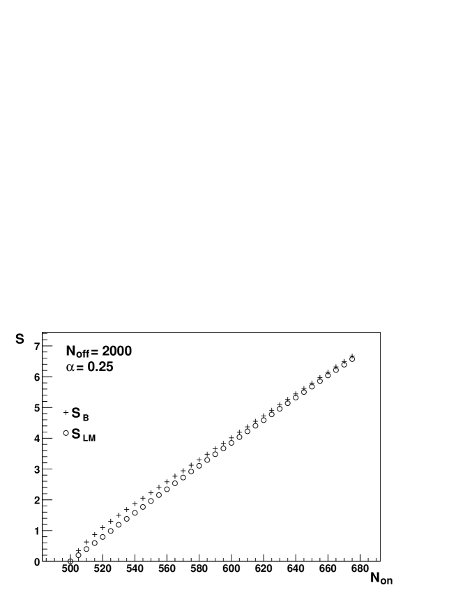
Figure 1:  Comparison of $S$ as a function of $N_{\mathrm{on}}$ for $\alpha=0.25$, $N_{\mathrm{off}}=2000$. Significance $S_{\mathrm{LM}}$ according to Li & Ma (circles) and Bayesian significance $S_{\mathrm{B}}$ (crosses)

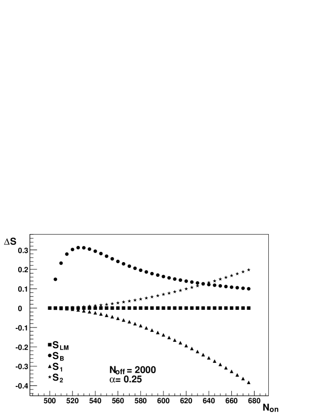
Figure 2:  Comparison of $S$ as function of $N_{\mathrm{on}}$ for $\alpha=0.25$, $N_{\mathrm{off}}=2000$. The difference $\Delta S=S-S_{\mathrm{LM}}$ is shown for $S=S_{\mathrm{B}}$ (dots) and the two estimates $S=S_{LM\,1}$ (equation (protect2), triangles) and $S=S_{LM\,2}$ (equation (3), stars).

For the calculation of the significance one needs the integral over $P_{1}$:

$$I_{1}(\omega) = \int_{\frac{\alpha}{\alpha+1}}^{\omega}P_{1}(v|N_{\mathrm{on}};N)\,dv$$

$$= \frac{N!\cdot\left(B_{\omega}\left(\frac{1}{2}+N_{\mathrm{on}},\frac{1}{2}+N_{\mathrm{off}}\right)-B_{\omega_{\mathrm{min}}}\left(\frac{1}{2}+N_{\mathrm{on}},\frac{1}{2}+N_{\mathrm{off}}\right)\right)}{\Gamma\left(\frac{1}{2}+N_{\mathrm{on}}\right)\,\Gamma\left(\frac{1}{2}+N_{\mathrm{off}}\right)-N!\cdot B_{\omega_{\mathrm{min}}}\left(\frac{1}{2}+N_{\mathrm{on}},\frac{1}{2}+N_{\mathrm{off}}\right)}\,.$$

The probability that a source has been detected is given by the probability that $\lambda_{\mathrm{s}}>0$. In the new parameters one wants to determine the confidence level to which one can exclude that $\omega$ equals its lower bound $\omega_{\mathrm{min}}$. Hence, one must solve the equation

$$p_{\mathrm{B}}(\omega_{\mathrm{up}})=p_{\mathrm{B}}(\omega_{\mathrm{min}})\,.$$ (29)

This cannot be solved analytically. However, one can prove that for $N_{\mathrm{on}},N_{\mathrm{off}}>0$ exactly one solution $\omega_{\mathrm{up}}\neq\omega_{\mathrm{min}}$ exists, since the binomial model has then a single maximum and no minima (see sect. D). With $\omega_{\mathrm{up}}$ the significance is

$$S_{\mathrm{B}}=\sqrt{2}\cdot\mathrm{erf}^{-1}(I_{1}(\omega_{\mathrm{up}}))\,,$$ (30)

where $\mathrm{erf}^{-1}$ is the inverse of the error function. Due to the appearance of $\omega_{\mathrm{up}}$ one cannot evaluate equation (30) any further. However, we can give a Mathematica script which calculates the Bayesian significance $S_{\mathrm{B}}$ in the described way (see sect. F). In figs. 1 and 2 the Bayesian significance is compared to the Li & Ma formula for a set of typical count numbers.

4 Large count numbers

4.1 Li & Ma

The procedure by Li & Ma is designed for the case of large count numbers. This is explicitely mentioned in the their paper (Li & Ma 1983) and it becomes apparent if one reparametrizes equation (4) in the following two variables:

$$N_{\mathrm{BG}} = \alpha\,N_{\mathrm{off}}$$ (31)

$$r = \frac{N_{\mathrm{on}}-N_{\mathrm{BG}}}{N_{\mathrm{BG}}}\,\,.$$ (32)

Here, $N_{\mathrm{BG}}$ is the count number expected in the on-region when no source is present and $r$ is the ratio of excess counts to the expected background. A positive significance requires $r>0$. Expressing $S_{\mathrm{LM}}$ in the observables $(N_{\mathrm{BG}},r)$ gives

$$S_{\mathrm{LM}}=\sqrt{2N_{\mathrm{BG}}}\,\left((1+r)\,\ln\frac{(1+r)(1+\alpha)}{1+\alpha+\alpha r}+\frac{1}{\alpha}\ln\frac{1+\alpha}{1+\alpha+\alpha r}\right)^{1/2}\,\,.$$ (33)

Hence, $S_{\mathrm{LM}}$ grows proportional to $\sqrt{N_{\mathrm{BG}}}$ as one would expect for significance. The point is that no other dependencies on $N_{\mathrm{BG}}$ are present, as the rest of equation (33) depends on the ratio of $r$ and $\alpha$ only.

4.2 Bayes

For the sake of comparison we must bring the Bayesian significance into the same form, such that its dependence on $N_{\mathrm{BG}}$ is the same as for $S_{\mathrm{LM}}$. That means that one has to take the limit of large $N_{\mathrm{BG}}$.
We can approximate the posterior distribution (eq. (27)) by a Gaussian for large count numbers. The apparent advantage is that this distribution can be treated analytically. The approximation is done best in the parameter in which the measure is uniform. Then the model and the posterior distributions are proportional to each other. Inspecting equation (24) shows that this happens for the parameter

$$\phi=\arcsin\left(\sqrt{\omega}\,\right)\,.$$ (34)

The approximation is calculated in appendix E. Using $\phi_{0}=\arctan(\sqrt{N_{\mathrm{on}}/N_{\mathrm{off}}})\,$ the result is

$$P_{2}(\phi|N_{\mathrm{on}};N)=\frac{1}{{\cal N}_{2}}\sqrt{\frac{2N}{\pi}}\exp\left(-2N\,(\phi-\phi_{0})^{2}\right)\,\,.$$ (35)

If ${\cal N}_{2}=1$, then $P_{2}$ is normalized in $]-\infty,\infty[$. The additional normalization factor ${\cal N}_{2}$ is due to the limited definition region of $\omega$, which means that $\phi$ is limited to

$$\phi_{\mathrm{min}}=\arcsin\left(\sqrt{\omega_{\mathrm{min}}}\,\right)\leq\phi\leq\frac{\pi}{2}\,\,.$$ (36)

It is handy to define the probability $K_{2}$ as if $\phi$ was defined on the entire real axis:

$$K_{2}=\int_{\phi_{\mathrm{min}}}^{\phi_{\mathrm{up}}}P_{2}(\phi|N_{\mathrm{on}};N)\,d\phi\left|\begin{array}[]{l}\\ {\cal N}_{2}=1\end{array}\right.\,\,,$$ (37)

The value of $K_{2}$ is

$$K_{2}=\mathrm{erf}\left(\sqrt{2N}\,(\phi_{0}-\phi_{\mathrm{min}})\right)\,\,.$$ (38)

The corresponding significance $S_{2}$ can easily be given as an analytical expression:

$$S_{2} = 2\sqrt{N}\,(\phi_{0}-\phi_{\mathrm{min}})$$ (39)

$$= 2\sqrt{N}\arcsin\frac{\sqrt{N_{\mathrm{on}}}-\sqrt{\alpha N_{\mathrm{off}}}}{\sqrt{(1+\alpha)N}}$$

$$= 2\sqrt{N_{BG}}\sqrt{\frac{1+\alpha+\alpha r}{\alpha}}\,\arcsin\frac{\sqrt{\alpha+\alpha r}-\sqrt{\alpha}}{\sqrt{(1+\alpha)(1+\alpha+\alpha r)}}\,\,.$$

The actual factor ${\cal N}_{2}$ will differ from unity. It is found by the condition

$$1=\int_{\phi_{\mathrm{min}}}^{\pi/2}P_{2}(\phi|N_{\mathrm{on}};N)\,d\phi\,\,.$$ (40)

For large count numbers the relevant range of $\phi$ is close to the position of the maximum, i.e. $\phi_{0}$. A crucial property of $P_{2}$ is that it does not vanish at $\phi_{\mathrm{min}}$. The value of $\phi_{0}$ is not far from $\phi_{\mathrm{min}}$. Therefore one can show that the upper limit of the integration in equation (40) can be replaced by infinity, as the corresponding correction vanishes exponentially with growing count numbers. Then one obtains

$${\cal N}_{2}=\frac{1}{2}\left(1+K_{2}\right)\,\,.$$ (41)

Note that ${\cal N}_{2}$ is close to unity, and it is necessarily smaller than unity. With the additional normalization factor ${\cal N}_{2}$ the integration over $P_{2}$ gives the Bayesian probability $K_{\mathrm{B}}$ in our approximation. Using the fact that $(1-K_{2})\ll 1$ one gets

$$K_{\mathrm{B}} = \frac{1}{{\cal N}_{2}}K_{2}=\frac{2K_{2}}{1+K_{2}}=\frac{1-(1-K_{2})}{1-(1-K_{2})/2}$$ (42)

$$\approx \left(1-\frac{}{}(1-K_{2})\right)\,\left(1+\frac{1-K_{2}}{2}\right)\approx 1-\frac{1-K_{2}}{2}=\frac{1+K_{2}}{2}$$

Going to the significance scale we have

$$\mathrm{erf}\left(\frac{S_{\mathrm{B}}}{\sqrt{2}}\right)=\frac{1}{2}\left(1+\mathrm{erf}\left(\frac{S_{2}}{\sqrt{2}}\right)\right)$$ (43)

Using equation (16) one gets

$$\frac{1}{S_{\mathrm{B}}}\exp\left(-\frac{S^{2}_{\mathrm{B}}}{2}\right)\approx\frac{1}{2}\,\frac{1}{S_{2}}\exp\left(-\frac{S^{2}_{2}}{2}\right)\,.$$ (44)

Setting $S_{\mathrm{B}}=(1+\delta)\,S_{2}$ and neglecting higher orders of $\delta$ yields

$$S_{\mathrm{B}}=S_{2}\cdot\left(1+\frac{\ln 2}{S_{2}^{2}}\right)\,\,.$$ (45)

The second term in this formula is due to the limited definition region of the source intensity parameter $\lambda$. With equation (39) one sees that its contribution becomes negligible for large $N_{BG}$ as it vanishes like $1/N_{BG}$. Then one simply has $S_{\mathrm{B}}=S_{2}$ which is plausible, as for large count numbers the distribution will become more and more concentrated around its maximum and therefore in the limit the definition region of the parameter no longer has an effect. So $S_{2}$ is the Bayesian expression which can be compared to the Li & Ma significance as given in equation (33). Apparently Bayesian inference and classical statistics also then yield different estimates for the significance.

5 Large count numbers and weak source

Typically, in gamma ray astronomy the detected sources are at the limit of the instruments’ sensitivities. Therefore long observation times are common. Thus the typical case is a weak source and large count numbers. The additional request of a weak source is expressed by the condition $r\ll 1$. In this limit the two significances actually do agree.

5.1 Li & Ma

Expanding the result in equation (33) up to the second order with respect to $r$ at $r=0$ gives

$$S_{\mathrm{LM}}\approx r\sqrt{\frac{N_{\mathrm{BG}}}{\alpha+1}}\,\left(1-\frac{2\alpha+1}{6\,(\alpha+1)}\,r\right)\,\,.$$ (46)

The expansion is done up to the order in which we encounter a difference to the Bayesian significance. Equation (46) is useful for small values of $r$. The first order term is sufficient if one requires that the second order term is small compared to the leading order. This gives the condition of how weak the source must be in that case:

$$r\ll\frac{6\,(1+\alpha)}{1+2\,\alpha}\,\,.$$ (47)

5.2 Bayes

Expanding the Bayesian result for large $N_{\mathrm{BG}}$ - hence $S_{2}$ in equation (39) - up to the second order with respect to $r$ at $r=0$:

$$S_{\mathrm{B}}=S_{2}\approx r\sqrt{\frac{N_{\mathrm{BG}}}{\alpha+1}}\,\left(1-\frac{1}{4}\,r\right)\,\,.$$ (48)

The first order is sufficient if $r\ll 1/4$.

5.3 Comparison

To first order in $r$, the formula given by Li & Ma agrees with the Bayesian result. The difference between the two significances is of second order in $r$:

$$S_{2}-S_{\mathrm{LM}}=r\sqrt{\frac{N_{\mathrm{BG}}}{\alpha+1}}\,\left(\frac{1}{12}\frac{\alpha-1}{\alpha+1}\,r\right)\,\,.$$ (49)

The numerical value of the fraction $(\alpha-1)/(\alpha+1)$ is always in $[-1,\,1]$. Together with the factor $1/12$ one finds therefore that the relative difference in significance is typically an order of magnitude smaller than the value of $r$. For $\alpha=1$ this relative difference is of order $r^{2}$. This shows that in the case of large count numbers and a weak source the Bayesian result and the formula given by Li & Ma are very close to each other.

Interestingly the correction due to the limited definition region (second term in equation (45)) is often numerically more important than the intrinsic difference between the two results as given by formula (49). For the case of $r=0.1$, $\alpha=0.3$ and a typical significance of $3\sigma$ the difference according to equation (49) is only of order 0.4%, whereas the limited definition region changes the significance by 6.9%. The correction by the restricted definition region is more important than the intrinsic difference given by the mathematically different treatment as long as

$$S^{2}\cdot r<12\,\ln 2\cdot\left|\frac{\alpha+1}{\alpha-1}\right|\,\,.$$ (50)

This case is relevant since the actual limit of large count numbers is hard to reach and it quickly leads to significances which are so high that one could not doubt the existence of a source. If condition (50) is fulfilled the difference between the two significances is dominated - technically speaking - by the definition region. The interesting point is that an unrestricted definition region would allow a source with negative intensity. Here, physics tells us that a source can only increase the count number since the source does not interfere with the background. In other words: An intensity always has a value $\geq 0$. One sees how Bayesian statistics allows us to take into account a-priori knowledge via the definition region. In classical statistics a-priori knowledge is not taken into account. Implicitely the intensity parameter of the source is completey free in $]-\infty,\infty[$.

Figure 3:  Difference $\Delta S=S-S_{\mathrm{LM}}$ for $\alpha=0.3$, $r=1/3$ as a function of $S_{\mathrm{LM}}$. The significance $S=S_{\mathrm{B}}$ (dots) is moderately higher than the one given by Li & Ma (squares). The curve shows $S=S_{\mathrm{B}}$ as calculated from the approximation given in equation (45). Note that the Bayesian procedure can only be evaluated for integer count numbers, not allowing for a continuous coverage on the $S_{\mathrm{LM}}$-axis. The off count number $N_{\mathrm{off}}$ varies from 0 to 2000 for $S_{\mathrm{LM}}$ from 0 to 7.5

6 Conclusions

The decision about a signal in the presence of background has been considered by Li & Ma in the framework of classical statistics. We have presented the Bayesian treatment of the same problem. This yields a complete solution which is not restricted to large count numbers. The Bayesian significance is correct for any $N_{\mathrm{on}}$, $N_{\mathrm{off}}$.
We compared the significance by Li & Ma with the Bayesian one in the limit of large count numbers. This was dictated by the fact that Li & Ma have formulated their expression for that limit. It turns out that classical statistics and Bayesian inference generally yield different results. They agree, however, in the limit of large count numbers and a weak source.
There are interesting cases where the limit of large count numbers is not fully reached. Then an accurate representation of the Bayesian significance requires a correction of order $N^{-1/2}$ as compared to the leading term which is of order $N^{1/2}$. There is no room for it in the argument of Li & Ma. The correction is due to the fact that a physical intensity parameter cannot have negative values. Bayesian inference takes care of this piece of prior knowledge.

Appendix A Calculation of measures

The evaluation of equation (9) is easy using the expectation values for the respective distribution. For the Poisson distribution one has

$$\left<n\right>_{\mathrm{P}} = \lambda\,,$$

$$\left<n^{2}\right>_{\mathrm{P}} = \lambda^{2}+\lambda\,.$$ (51)

For the binomial distribution the expectation values are

$$\left<n\right>_{\mathrm{B}} = N\,\lambda\,,$$

$$\left<n^{2}\right>_{\mathrm{B}} = N\,\lambda\,((N-1)\,\lambda+1)\,.$$ (52)

The measure of the Poisson distribution is therewith:

$$\ln p_{\mathrm{P}}(n|\lambda) = n\,\ln\lambda-\lambda\,,$$

$$\partial_{\lambda}\ln p_{\mathrm{P}}(n|\lambda) = \frac{n}{\lambda}-1\,,$$

$$\left<\left(\partial_{\lambda}\ln p_{\mathrm{P}}(n|\lambda)\right)^{2}\right>_{\mathrm{P}} = 1-2+\frac{1+\lambda}{\lambda}=\frac{1}{\lambda}\,,$$

$$\mu_{\mathrm{P}}(\lambda) = \lambda^{-1/2}\,.$$ (53)

The measure of the binomial distribution is

$$\ln p_{\mathrm{B}}(n|\lambda;N) = \ln{N\choose n}+n\ln\lambda+(N-n)\ln(1-\lambda)\,,$$

$$\partial_{\lambda}\ln p_{\mathrm{B}}(n|\lambda;N) = \frac{n}{\lambda}-\frac{N-n}{1-\lambda}\,,$$

$$\left<\left(\partial_{\lambda}\ln p_{\mathrm{B}}(n|\lambda;N)\right)^{2}\right>_{p_{\mathrm{B}}} = \frac{N}{\lambda(1-\lambda)}\,,$$

$$\mu_{\mathrm{B}}(\lambda) = \left(\frac{N}{\lambda(1-\lambda)}\right)^{1/2}\,.$$ (54)

The conditional measure $\mu_{0}(\lambda_{\mathrm{off}}|\lambda_{\mathrm{s}})$ needed in equation (20) is calculated in the same way, using the expectation values for the Poisson distribution:

$$\ln p_{0}(N_{\mathrm{on}},N_{\mathrm{off}}|\lambda_{\mathrm{s}},\lambda_{\mathrm{off}}) = N_{\mathrm{on}}\ln(\lambda_{\mathrm{s}}+\alpha\lambda_{\mathrm{off}})-\lambda_{\mathrm{s}}-\alpha\lambda_{\mathrm{off}}+$$

$$N_{\mathrm{off}}\ln\lambda_{\mathrm{off}}-\lambda_{\mathrm{off}}-\ln(N_{\mathrm{off}}!\,N_{\mathrm{on}}!)\,,$$

$$\partial_{\lambda_{\mathrm{off}}}\ln p_{0}(N_{\mathrm{on}},N_{\mathrm{off}}|\lambda_{\mathrm{s}},\lambda_{\mathrm{off}}) = \frac{\alpha\,N_{\mathrm{on}}}{\lambda_{\mathrm{on}}}-\alpha+\frac{N_{\mathrm{off}}}{\lambda_{\mathrm{off}}}-1\,,$$

$$\left<\left(\partial_{\lambda_{\mathrm{off}}}\ln p_{0}(N_{\mathrm{on}},N_{\mathrm{off}}|\lambda_{\mathrm{s}},\lambda_{\mathrm{off}})\right)^{2}\right>_{p_{0}} = \frac{\alpha^{2}}{\lambda_{\mathrm{on}}}+\frac{1}{\lambda_{\mathrm{off}}}\,,$$

$$\mu_{0}(\lambda_{\mathrm{off}}|\lambda_{\mathrm{s}}) = \left(\frac{\alpha^{2}}{\alpha\lambda_{\mathrm{off}}+\lambda_{\mathrm{s}}}+\frac{1}{\lambda_{\mathrm{off}}}\right)^{1/2}\,.$$ (55)

Appendix B Check if the minor model is proper

It has to be checked whether the model $q_{0}$ in equation (20) is proper. Thus one has to evaluate

$$\sum_{N_{\mathrm{on}},\atop N_{\mathrm{off}}}q_{0}(N_{\mathrm{on}},N_{\mathrm{off}}|\lambda_{\mathrm{s}}) = \sum_{N_{\mathrm{on}},\atop N_{\mathrm{off}}}\int_{0}^{\infty}p_{0}(N_{\mathrm{on}},N_{\mathrm{off}}|\lambda_{\mathrm{s}},\lambda_{\mathrm{off}})\,\mu_{0}(\lambda_{\mathrm{off}}|\lambda_{\mathrm{s}})\,d\lambda_{\mathrm{off}}$$ (56)

$$= \int_{0}^{\infty}\mu_{0}(\lambda_{\mathrm{off}}|\lambda_{\mathrm{s}})\,d\lambda_{\mathrm{off}}$$

$$= \int_{0}^{\infty}\left(\frac{\alpha^{2}}{\alpha\lambda_{\mathrm{off}}+\lambda_{\mathrm{s}}}+\frac{1}{\lambda_{\mathrm{off}}}\right)^{1/2}\,d\lambda_{\mathrm{off}}\,.$$

This integral diverges and hence $q_{0}(N_{\mathrm{on}},N_{\mathrm{off}}|\lambda_{\mathrm{s}})$ is an improper model.

Appendix C Transformation to a proper model

The transformation from the original parameters $(\lambda_{\mathrm{s}},\lambda_{\mathrm{off}})$ to the new ones $(\omega,\Lambda)$ is calculated in a few lines:

$$p_{0}(N_{\mathrm{on}},N_{\mathrm{off}}|\lambda_{\mathrm{s}},\lambda_{\mathrm{off}}) \stackrel{{\scriptstyle(\ref{p0})}}{{=}} \frac{\lambda_{\mathrm{on}}^{N_{\mathrm{on}}}}{N_{\mathrm{on}}!}\,e^{-\lambda_{\mathrm{on}}}\,\frac{\lambda_{\mathrm{off}}^{N_{\mathrm{off}}}}{N_{\mathrm{off}}!}\,e^{-\lambda_{\mathrm{off}}}$$ (57)

$$= \frac{(\Lambda\,\omega)^{N_{\mathrm{on}}}}{N_{\mathrm{on}}!}\,\frac{(\Lambda(1-\omega))^{N_{\mathrm{off}}}}{N_{\mathrm{off}}!}\,e^{-\Lambda}$$

$$= \Lambda^{N}\,e^{-\Lambda}\,\frac{1}{N_{\mathrm{on}}!\,N_{\mathrm{off}}!}\,\omega^{N_{\mathrm{on}}}(1-\omega)^{N_{\mathrm{off}}}$$

$$= \frac{\Lambda^{N}\,e^{-\Lambda}}{N!}\,{N\choose N_{\mathrm{on}}}\,\omega^{N_{\mathrm{on}}}(1-\omega)^{N-N_{\mathrm{on}}}$$

$$\stackrel{{\scriptstyle(\ref{poisson}),(\ref{binomial})}}{{=}} p_{\mathrm{P}}(N|\Lambda)\cdot p_{\mathrm{B}}(N_{\mathrm{on}}|\omega;N)\,.$$

Appendix D Uniqueness of the solution

The first derivative of the model $p_{\mathrm{B}}$ from equation (6) is

$$p^{\prime}_{\mathrm{B}}(\omega|N_{\mathrm{on}};N)=\left(\frac{N_{\mathrm{on}}}{\omega}-\frac{N_{\mathrm{off}}}{1-\omega}\right)\,p_{\mathrm{B}}(\omega|N_{\mathrm{on}};N)\,.$$ (58)

It vanishes at

$$\omega_{0}=\frac{N_{\mathrm{on}}}{N}\,.$$ (59)

The value of the second derivative at $\omega_{0}$ is

$$p^{\prime\prime}_{\mathrm{B}}(\omega_{0}|N_{\mathrm{on}};N)=-\frac{N^{3}}{N_{\mathrm{off}}\,N_{\mathrm{on}}}<0\,.$$ (60)

Hence, $p_{\mathrm{B}}$ has a single maximum and no minima. Therefore for each $\omega_{1}\neq\omega_{0}$ one has exactly one other $\omega_{2}$ for which equation (29) holds. Thus one has a unique solution $\omega_{\mathrm{up}}\neq\omega_{\mathrm{min}}$ in equation (29).

Appendix E Approximation to the posterior distribution

The result of the transformation of $p_{\mathrm{B}}(\omega)$ to the parameter $\phi=\arcsin(\sqrt{\omega})$ is

$$p_{\phi}(\phi)\sim(\sin\phi)^{2N_{\mathrm{on}}}\,(\cos\phi)^{2N_{\mathrm{off}}}\,.$$ (61)

The approximation is achieved by expanding the logarithm of the distribution around its maximum and taking the exponential of the result. Using $\gamma=N_{\mathrm{on}}/N_{\mathrm{off}}=\alpha\,(1+r)\,$ the maximum is at

$$\phi_{0}=\arctan\left(\sqrt{\gamma}\,\right)\,.$$ (62)

The expansion up to second order is

$$\ln p_{\phi}(\phi)=C_{1}(N_{\mathrm{on}},N)-2N\,\left(\phi-\phi_{0}\right)^{2}+O[\phi^{3}]\,.$$ (63)

Hence, one has

$$\tilde{P_{2}}=\frac{1}{C_{2}}\exp\left(-2N(\phi-\phi_{0})^{2}\right)$$ (64)

With the normalization constant

$$C_{2}=\sqrt{\frac{\pi}{2N}}$$ (65)

the distribution $P_{2}$ is normalized in $]-\infty,\infty[$.

Appendix F Mathematica script to evaluate Bayesian significance

Although we cannot give a close formula for the Bayesian significance, we can show a short Mathematica script which calculates the significance as given in equation (30).

data = {   a -> 0.25,
         non -> 16,
        noff -> 10 };

n = non + noff;
b = non/noff;
wmin = a/(1 + a);
pBin[x_, n_, non_] := Binomial[n, non]x^non(1 - x)^(n - non);
pRaw[x_, n_, non_] := pBin[x, n, non] (Sqrt[n/x(1 - x)]);
norm = Integrate[pRaw[x, n, non], {x, wmin, 1}];
p[x_] := pRaw[x, n, non]/norm;
rule =  FindRoot[Evaluate[(1 - w) (1 + a)  == (wmin/w)^b /.data],
                 {w, wmin/a, non/n, 1}/.data];
i[w0_, w1_] := Integrate[p[w], {w, w0, w1}, GenerateConditions -> False];
temp = Evaluate[(i[wmin, w /. rule]) /. data];

Print["Sigma (Bayes): "];
sigma = InverseErf[temp] Sqrt[2]

References

- Li & Ma (1983) Li, T. & Ma, Y. 1983, ApJ, 272, 317
- Harney (2003) Harney, H. L. 2003, Bayesian inference (Heidelberg: Springer-Verlag Berlin Heidelberg)
- Jeffreys (1961) Jeffreys, H. 1961, Theory of probability, (3d ed.; Oxford: Oxford University Press)
- Bernardo (1979) Bernardo, J. M. 1979, J. Roy. Statist. Soc., B41, 113
- Dawid (1973) Dawid, A. P., Stone, N., Zidek, J. V. 1973, J. Roy. Statist. Soc., B35, 189