A method of generating initial conditions for cosmological N body simulations

Abstract

We investigate the possibility of generating initial conditions for cosmological N-body simulations by simulating a system whose correlations at thermal equilibrium approximate well those of cosmological density perturbations. The system is an appropriately modified version of the standard “one component plasma” (OCP). We show first how a well-known semi-analytic method can be used to determine the potential required to produce the desired correlations, and then verify our results for some cosmological type spectra with simulations of the full molecular dynamics. The advantage of the method, compared to the standard one, is that it gives by construction an accurate representation of both the real and reciprocal space correlation properties of the theoretical model. Furthermore the distributions are also statistically homogeneous and isotropic. We discuss briefly the modifications needed to implement the method to produce configurations appropriate for large N-body simulations in cosmology, and also the generation of initial velocities in this context.

I INTRODUCTION

One of the major goals of current models in cosmology is to link the very small amplitude fluctuations observed in the cosmic microwave background to the large inhomogeneities observed today in the distribution of galaxies. The former should serve as the initial seeds for the formation of the large structures observed, in the available time, through the attraction of gravity. In the absence of a full analytic understanding of the problem, gravitational N-body simulation has become an essential instrument in making this link (for reviews, see e.g. EDFW , white , couchman ). In this paper we are concerned with one element of N-body simulation: the setting up of appropriate initial conditions (IC).

The theoretical IC for such simulations are specified by the cosmological model considered, which gives the correlation properties, at the initial time of the simulation, of a continuous stochastic mass density field $\rho(\vec{r})$. This field has a well defined mean density $\rho_{0}(>0)$, and fluctuations $\delta_{\rho}(\vec{r})=\rho(\vec{r})/\rho_{0}-1$, which are of small amplitude an generically assumed to be Gaussian. The correlation properties are thus fully specified by the power spectrum (PS) of the model. The subtlety in the generation of the IC for an N-body simulation is in the fact that a realization of this theoretical stochastic density field, which is a continuous function, must be discretised: it must be represented by an initial distribution in space of the N point particles used in the simulation. The correlation properties of these two qualitatively different kinds of distributions, however, cannot be the same. At small scales, in particular, the discrete distribution has density fluctuations with infinite variance (points), while the continuous model has finite variance fluctuations at all scales. The correlation properties of the set of N discrete particle must, nevertheless, approximate, in some appropriate sense, those of the theoretical model.

There is one well known and universally employed method for generating the IC of N body simulations. It uses the so-called “Zeldovich approximation” zel ; buchert . Particles are displaced off a perfect lattice (or sometimes “glassy”) configuration in a manner determined by the desired theoretical PS. Thus every realization of the theoretical stochastic density field is mapped onto an initial configuration of the N particles. Each such configuration can thus be considered as a realizaion of a discrete stochastic density field.

Usually the characterisation of the correlation properties of this discrete distribution (i.e. of the generated discrete IC) are considered only in reciprocal space, i.e. in terms of a measured PS, which approximates well the PS of the input theoretical model for sufficiently small $k$ (i.e. small compared to the Nyquist frequency characteristic of the discreteness of the underlying lattice). The question of the representation of real space correlation properties (e.g. mass variance in spheres and the two point correlation function) has been the subject of some discussion in the recent literature . A detailed study of this question is presented in a recent article by two of us jm04 . The standard method is shown rigorously to give a distribution with a PS approximating well that of the input theoretical model below the Nyquist frequency of the lattice, for quite a broad class of input PS . In real space, however, it can be shown that the correlation properties are generically a mixture, at all scales, between those of the underlying lattice and those of the theoretical model. The real space correlation function carries, notably, the trace of the underlying oscillating behaviour of the initial lattice correlation function. The mass variance in a sphere is also typically dominated by that of the lattice to scales which, depending on the input theoretical model and its normalisation, can be very much larger than the interparticle spacing.

The question which inevitably follows is whether such a discrepancy between the correlation properties of the theoretical model and those of its discretisation are important for what concerns the interpretation of the results of the dynamical evolution of the discrete N-body simulation under gravity. These evolved configurations are taken to represent, over a very wide range of scale (typically from well below the initial inter-particle separation up to scales a little smaller than the size of the periodic box), the evolution of a continuous self-gravitating fluid with the initial theoretical correlation properties. Is it sufficient to have only a faithful representation of the initial correlation properties in reciprocal space? This is an open question, which we do not attempt to answer here. In order to answer it, however, it would evidently be useful to have other methods for generating discrete representations of the theoretical IC. More generally, for the study of gravitational evolution from near homogeneous IC, it is of interest to have a diversity of methods for generating initial configurations.

The aim of this work is to explore a possible such method which has been suggested in gjjlpsl02 . The idea is simple: to find a system whose dynamics produces configurations with the required correlation properties. Given that the IC describe very small fluctuations about homogeneity, it is natural to seek a system whose thermal equilibrium gives rise to such configurations. In gjjlpsl02 it has been noted that a simple modification of the interparticle potential in the “one component plasma” (OCP), which is a well-known and much studied system in statistical physics, gives rise to a PS at small wavenumbers which is identical to that of cosmological models, with fluctuations which are also Gaussian. Further it is argued qualitatively in gjjlpsl02 that an appropriate modification of this potential at smaller scales could give rise to the correlations typical of standard “cold dark matter” (CDM) cosmologies (which are of the class currently favoured by cosmologists). In this paper we show how a well known semi-analytic method, the hypernetted chain (HNC), for determining the correlation properties of such systems at equilibrium can be adapted to allow one to infer the required interaction potential given an input spectrum. We apply this inversion for some simple model CDM-type spectra, and find a potential with the qualitative features anticipated by gjjlpsl02 . We then verify the accuracy of this method with a simulation of the full molecular dynamics. This involves modifying the Ewald sum method for calculation of the potential.

The paper is organised as follows. In the next section we discuss first the important underlying question of how the correlation properties of a continuous field may be represented by a discrete distribution. In section III we briefly recall the basic features of the standard OCP, and explain the analytical statistical mechanics approach to the determination of its correlation properties. In particular we describe the HNC approximation which gives a closed form for the determination of the two point correlation properties from the potential. We explain how it can be used in an inverted form to infer the required inter-particle potential for an input (physically reasonable) correlation function. We show then how this can be done for a CDM type spectra, giving numerical results for some cases. In the next section we turn to the simulation of the molecular dynamics of these systems. We give results for several simulations which verify the results anticipated from the HNC, and provide actual realizations of discretisations of CDM type spectra. In the final section we discuss the possibility of using this method to generate configurations representing the IC of cosmological NBS, as in principle the method appears to work well and to provide an interesting, and perhaps more satisfactory, alternative to the standard algorithm. One issue is the generation of appropriate initial velocities. We explain that this can be done as in the standard method, as the Zeldovich approximation gives a relation between the initial particle velocity and the gravitational field acting on it, which can also be applied to our configurations. A more non-trivial issue is that of the size of the configurations generated: the simulations we have performed to test the viability of the method are of a quite modest size — the largest simulation reported here has slightly less than 9000 particles — while current cosmological simulations use, at the very least, hundreds of thousands of particles. Just as in the case of NBS itself, it will be necessary to speed up the algorithm developed here to attain this goal. The methods for this latter step already exist and can be applied to the more complicated two body potentials we study.

II REPRESENTATION OF CONTINUOUS SPECTRA WITH POINT DISTRIBUTIONS

II.1 Discrete and continuous stochastic density fields

Let us first recall (see e.g. pee80 , gsljp-springer ) some basic properties of the PS (or, in the terminology more common in statistical physics, structure function). We will use $P(\vec{k})$ to denote this quantity when we refer to a continuous distribution, $S(\vec{k})$ for the discrete case. For both cases it can be defined as

$$P(\vec{k})=\lim_{V\rightarrow\infty}\frac{\langle|\delta_{\rho}(\vec{k})|^{2}\rangle}{V}$$ (1)

where $\delta(\vec{k})$ is the Fourier Transform (hereafter FT) of the normalized fluctuation field $(\rho(\vec{r})-\rho_{0})/\rho_{0}$, and the angle brackets indicate an ensemble average. We will assume that the system is statistically isotropic so the PS will not depend on the orientation of the vector $\vec{k}$ i.e. $P(\vec{k})=P(k)$. We will also assume statistical homogeneity (i.e. invariance of average quantities under translation). In this case the Fourier transform of the PS, for which we use the convention

$$\xi(\vec{r})=\frac{1}{(2\pi)^{3}}\int d^{3}ke^{i{\vec{k}}{\vec{r}}}P(\vec{k})\,,$$ (2)

is the reduced two point correlation function defined as

$$\xi(\vec{r})\equiv\xi(r)=\frac{\langle\rho(r)\rho(0)\rangle}{\langle\rho(0)\rangle^{2}}-1=\langle\delta_{\rho}(r)\delta_{\rho}(0)\rangle\,.$$ (3)

The intrinsic difference between a continuous and discrete density field $\rho(\vec{r})$ manifests itself in a qualitative difference between the mathematical properties of the two-point quantities in each case. In real space the correlation function $\xi(\vec{r})$ has, for the class of finite one-point variance continuous fields which we consider, the property

$$-1\leq\xi(r)\leq\xi(0)<\infty\,.$$ (4)

For the discrete case the one-point variance, which is equal to $\xi(0)$, necessarily diverges because of the singular nature of the density field at any point. The correlation function can then be written

$$\xi(r)=\frac{1}{n_{0}}\delta(\vec{r})+h(r)$$ (5)

where $n_{0}$ is the mean number density, $\delta(\vec{r})$ is the (three dimensional) Dirac delta function, and $h(r)$ is a non-singular function for all $r$ which can be taken to have the property analogous to Eq.(4).

These properties in real space translate in $k$ space into a difference in the asymptotic properties of the power-spectra at large $k$. The one-point variance of the density field is also given by the integral of the PS, and so for the continuous case we have

$$\lim_{k\rightarrow\infty}k^{3}P(k)=0$$ (6)

in order that this variance be finite. In the discrete case, on the other hand, we have

$$\lim_{k\rightarrow\infty}S(k)=\frac{1}{n_{0}}$$ (7)

$$\lim_{k\rightarrow\infty}k^{3}(S(k)-\frac{1}{n_{0}})=0\,.$$ (8)

i.e. the divergence of the one-point variance is entirely associated to the “Poissonian” term in the PS, which is simply the FT of the delta-function singularity in real space explicit in Eq.(5). Note that both $P(k)$ and $S(k)$ are, by definition, positive functions, while $S(k)-\frac{1}{n_{0}}$ is not. There is therefore no bound $S(k)\geq 1/n_{0}$. In particular, one can have $S(k)\rightarrow 0$ for $k\rightarrow 0$, in systems satisfying the constraint

$$\int d^{3}rh(r)=-\frac{1}{n_{0}}\,$$ (9)

i.e. when there is appropriate anti-correlation to balance the contribution to fluctuations at all scales from the Poissonian term associated to any discrete process. As discussed in gjjlpsl02 , gsljp-springer , glass these correspond to highly ordered “super-homogeneous” systems.

II.2 Smoothing of discrete distributions

The intuitively evident fact that a discrete distribution can only represent the correlation properties of a continuous field above some scale — that characteristic of the “granularity” of the discrete distribution — is reflected mathematically in the differences just discussed between the properties in the two cases of the correlation function at small real space separations, and the PS at large wave-numbers. Let us suppose now that we have a discrete distribution with PS $S(k)$, and a continuous distribution with PS $P(k)$. What is meant when one says that the former is a discretisation of the latter? In what sense can we say that the former represents the correlation properties of the continuous distribution with PS $P(k)$? The answer to this question is that there is in fact no unique prescription for passing between a discrete and continuous distribution. In particular taking formally the limit in which the number of particles goes to infinity at fixed mass density, which one might naively think to define the desired continuous limit, does not do so. Consider, for example, the case of an (uncorrelated) Poisson point process: as the number density is taken to infinity the fluctuations also go to zero. Thus the continuous limit is an exactly uniform distribution with $P(k)=0$.

As discussed in gjjlpsl02 the most natural way of defining such a relationship is by an appropriate local smoothing i.e. we assume the represented density field is given by the convolution of the discrete distribution with a spatial window function $W_{R_{s}}(r)$

$$\rho_{c}(\vec{r})=\int W_{R_{s}}(|\vec{r}-\vec{r}\,^{\prime}|)\rho_{d}(\vec{r}\,^{\prime})d^{3}\vec{r}\,^{\prime}$$ (10)

where $R_{s}$ is the (single) characteristic smoothing scale and the realization of the discrete field is a sum over all the particles

$$\rho_{d}(\vec{r})=\sum_{i}\delta(\vec{r}-\vec{r}_{i})\,,$$ (11)

and $\rho_{c}(\vec{r})$ is the corresponding realization of the continuous stochastic density field. We then have that

$$P(k)=|\tilde{W}_{R_{s}}(k)|^{2}S(k)$$ (12)

where $\tilde{W}_{R_{s}}(k)$ is the Fourier transform of $W_{R_{s}}(r)$. By the assumption that the window function gives a local smoothing, we mean that it is an integrable function. It is naturally normalised to unity (to conserve mass) so that $\tilde{W}_{R_{s}}(0)$ is equal to unity. Thus the PS of the discrete field must approximate well that of the continuous one for small $k$ (i.e. $k\ll R_{s}^{-1}$). In real space the smoothing leads to the convolution relation

$$\xi_{c}(r)=\int W_{R_{s}}(\vec{r}\,^{\prime})W_{R_{s}}(\vec{r}\,^{\prime\prime})\xi_{d}(\vec{r}+\vec{r}\,^{\prime}-\vec{r}\,^{\prime\prime})d^{3}\vec{r}\,^{\prime}d^{3}\vec{r}\,^{\prime\prime}$$ (13)

between the continuous correlation function $\xi_{c}(r)$ and the discrete correlation function $\xi_{d}(r)$. One sees explicitly how the singularity becomes regularised applying (13) to (5):

$$\frac{1}{n_{0}}\delta(\vec{r})\to\frac{1}{n_{0}}\int W_{R_{s}}(\vec{r}\,^{\prime})W_{R_{s}}(\vec{r}+\vec{r}\,^{\prime})d^{3}\vec{r}\,^{\prime}.$$ (14)

Note that any pair consisting of a discrete and a continuous density field, with PS $P(k)$ and $S(k)$ respectively, can be related to one another formally by Eq.(12), taken simply as a definition of the smoothing function . Whether $S(k)$ can be considered to be a physically reasonable discretisation of $P(k)$ depends then on the mathematical properties of this smoothing function i.e. whether it really represents a physical smoothing. It is useful, for what follows, to express the relation between the two spectra in a slightly different (but equivalent) form:

$$S(k)=P(k)+\frac{1}{n_{0}}D(k)$$ (15)

where $n_{0}$ is the number density of the discrete distribution, The function $D(k)$ has then the properties imposed by Eqs.(7) and (8):

$$\lim_{k\rightarrow\infty}D(k)=1$$ (16)

$$\lim_{k\rightarrow\infty}k^{3}(D(k)-1)=0\,.$$ (17)

In real space one has analogously

$$h(r)=\xi_{c}(r)-\frac{1}{n_{0}}FT[1-D(k)]$$ (18)

where $\xi_{c}(r)$ is the Fourier transform of $P(k)$ i.e. the reduced two-point correlation function of the continuous model. Expressed in terms of the smoothing we have from Eq.(12) that

$$|\tilde{W}_{R_{s}}(k)|^{-2}=1+\frac{D(k)}{n_{0}P(k)}\,.$$ (19)

Note that whether the smoothing which is associated to a $D(k)$ is a physical smoothing depends, therefore, not only on its own properties, but also on those of $P(k)$.

II.3 Discretisation in the standard algorithm

The standard method for generating IC for N-body simulations in cosmology superimposes correlated displacements on a “pre-initial” configuration of points representing “uniformity”. The latter is usually taken to be a perfect lattice, but sometimes also a “glassy” configuration obtained by running the N-body code with the sign of gravity reversed (i.e. with Coulomb forces) and an appropriate damping term. Both of these configurations represent an unstable equilibrium point (approximately in the latter case) under their self-gravity, and evolve only when the perturbations are applied. The precise sense in which this method leads to a representation of the continuous model (and whether this is adequate for the dynamics which is simulated) is not discussed in the literature, but implicitly the criterion used appears to be

$$S(k)\approx P(k)\quad{\rm for}\quad k<k_{d}$$ (20)

where $k_{d}$ is the wave-number characteristic of the discreteness (i.e. the Nyquist frequency in the case of the lattice). In jm04 we have investigated systematically the real and reciprocal space correlation properties of configurations generated by this algorithm, using a formalism developed in gab04 . We give, in particular, exact expressions for the PS $S(k)$ of the generated distribution, for a given input theoretical PS $P(k)$. From this one can infer explicitly the form of $D(k)$, as defined in Eq.(15), and the corresponding “smoothing” given through Eq.(19). The essential point is that $D(k)$ carries all the correlation of the “pre-initial” configuration. Indeed one has, to a first approximation, simply that $D(k)\approx n_{0}P_{in}(k)$ where $P_{in}(k)$ is the PS of the “pre-initial” (lattice or glass) configuration.In $k$-space this correlation is “localised” at large $k$, so that Eq.(20) is satisfied. In real space, however, the second term on the right hand side of Eq. (18 is not localised to below the inter-particle distance, and completetly dominates the small amplitude correlations of the input model . Correspondingly the algorithm generically does not give a discretisation which can be interpreted as a localised smoothing in the sense we have discussed above: the function $W_{R_{S}}(r)$ determined through Eq.(12) (or, equivalently, Eq.(19) is also highly delocalised). This is simply because the underlying regularity of the “pre-initial” configuration, which is not a feature of the continuous model, cannot be removed by a localised smoothing.

II.4 Determination of the PS of a new discretisation

We investigate here a different method for discretising a given input PS $P(k)$. The principle is to seek to generate a distribution with an $S(k)$ given through Eq.(15), where for $D(k)$ we will choose a smooth function of $k$, characterised by a single scale $k_{d}$, and interpolating between zero for $k<k_{d}$ and unity for $k>k_{d}$ (and in keeping with the asymptotic properties required Eqs.(16) and (17)). The scale $k_{d}$ will be chosen of order the inverse of the mean particle separation $a$ (see below for the exact definition we use). Further the function $D(k)$ will be such that the FT of $(D(k)-1)$ in Eq.(18) is localised strongly in real space on the scale $a$. Thus, by construction, we will converge to

$$S(k) \approx P(k)\quad{\rm for}\quad k\ll k_{d}$$ (21)

$$h(r) \approx \xi_{c}(r)\quad{\rm for}\quad r\gg a$$ (22)

As we have noted, whether this choice of $D(k)$ corresponds to a physical smoothing, in the sense we have discussed, depends also on the properties of $P(k)$. For the well-behaved $P(k)$ we will consider we expect this to be the case, but we will check explicitly that the function $W_{R_{s}}(r)$ is smooth and integrable.

The precise scale $k<k_{d}$ at which Eq.(21) holds will depend both on $D(k)$ and on the form and normalisation of the PS. In the cosmological context $P(k)$ is generically a monotonically decreasing function over a wide range of $k$ for $k<k_{d}$, and thus the dimensionless quantity $n_{0}P(k_{d})$ gives a parametrisation of the relative amplitudes of the “continuous” and “discrete” parts of the full PS $S(k)$. In the simulations of molecular dynamics described below we will take $n_{0}P(k_{d})\sim 1$. Thus we will have in this case Eq.(21) for all $k\raise 1.72218pt\hbox{$<$}\kern-8.00003pt\lower 2.6694pt\hbox{$\sim$}k_{d}$, and (we will verify) Eq.(22) from $r\raise 1.72218pt\hbox{$>$}\kern-6.99997pt\lower 2.6694pt\hbox{$\sim$}a$ .

In our explicit examples of the construction of $S(k)$ we will make the simple choice $D(k)=1-e^{-k^{2}/2k_{d}^{2}}$, which evidently has the required asymptotic properties. It is important to note that we have not shown that the $S(k)$ then given by Eq.(15) and such a choice of $D(k)$ is necessarily the PS of a real discrete distribution . Indeed it is easy to see that the ansatz for $S(k)$ may be unrealizable in a discrete distribution: we have noted that the two-point correlation function $h(r)$ of the discrete distribution must satisfy by definition $h(r)\geq-1$. Taking Eq.(18), it is not difficult to verify that this condition places an upper bound on $k_{d}$, of order the inverse of the average inter-particle distance . Physically it is very reasonable that such a bound arises: taking $k_{d}$ larger than the inverse of the inter-particle separation one is requiring the discrete distribution to mimic the correlation properties of the continuous model in a regime where the intrinsic difference in the nature of the distributions is important.

III SEMI-ANALYTIC DETERMINATION OF THE POTENTIAL: THE HNC

In this section we discuss first the OCP and a standard method use to determine its correlation properties. The inversion of this method to determine the potential which would be expected to give reasonable desired input correlation properties is then explained.

III.1 The standard OCP

The OCP (for a review, see baus_1980 ) is a system of positive charged point particles (“ions”) interacting through a Coulomb (i.e. repulsive $1/r$) potential, and embedded in a uniform (rigid, non-dynamical) negatively charged background . The latter gives overall charge neutrality, and a high degree of stability to the system. The system exhibits two phases at thermal equilibrium, a fluid phase and a solid phase. We will treat it always at densities and temperatures where it is in the fluid phase. In this range of densities and temperature it can be considered as completely classical.

The equilibrium thermodynamics of the OCP is determined by a single parameter, and not by its temperature and density independently. Because of the scale-free nature of the power-law interaction potential, there are only two characteristic length scales. One is specified by the number density, and is conventionally taken to be the “ion-sphere” (or simply ionic) radius $a$ defined by

$$a=\left(\frac{3}{4\pi n}\right)^{1/3}$$ (23)

where $n=N/V$ is the number density of the $N$ points in a volume $V$. The other scale is given by the distance at which the potential is of order the mean thermal kinetic energy. It is the dimensionless ratio of these two scales which parametrises the one dimensional phase space of the system at thermal equilibrium. Conventionally this parameter is taken to be

$$\Gamma=\beta(Ze)^{2}/a.$$ (24)

where $\beta=1/(k_{B}T)$ and $Ze$ is the ionic charge. It is refered to as the “plasma parameter” (or simply “coupling constant”).

Numerical calculations are necessary to compute reliably the correlation properties of the OCP. The correlation function $g(r)$ (defined as $g(r)=h(r)+1$) and PS $S(k)$ are shown in Figs. 1 and 2 for different values of the coupling $\Gamma$.

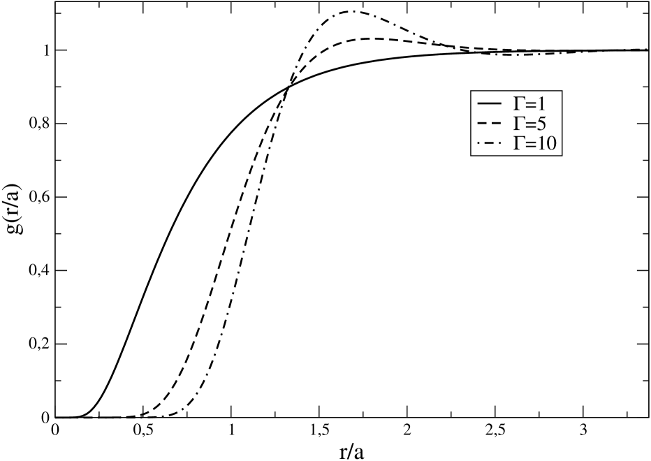
Figure 1: Correlation function of the OCP with interacting Coulomb potential for different temperatures (recall that $\Gamma\sim 1/T$).

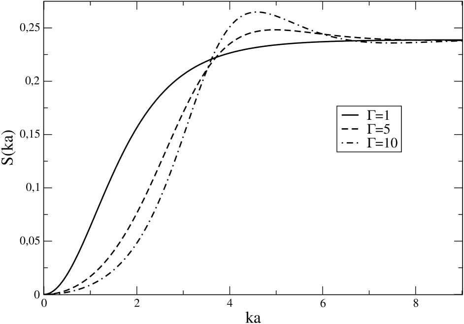
Figure 2: Power spectrum of the OCP with interacting Coulomb potential. Note that this is a linear-linear plot.

In the weak coupling limit ($\Gamma\ll 1$ i.e. high temperature/low density) the OCP can be shown to have two point correlations given approximately as

$$h(r)\equiv\left(g(r)-1\right)\sim-\beta\frac{e^{-\kappa r}}{r},\quad\kappa^{2}=4\pi Z^{2}e^{2}\beta n.$$ (25)

i.e. exponentially decaying anti-correlations. This is simply a manifestation of screening, and $\kappa^{-1}$ is the Debye length:

$$\lambda_{D}=(4\pi Z^{2}e^{2}n\beta)^{-1/2}=\frac{a}{\sqrt{3\Gamma}}.$$ (26)

Particles are repelled locally around a given particle in such a way that the effective potential due to a particle decays exponentially in this way. At larger values of $\Gamma$ (i.e. lower temperature/higher density) one sees that the correlation function develops a “bump” at small scales, indicating that the first neighbour is becoming increasingly localised. As $\Gamma$ increases further several “bumps” develop (corresponding to first, second, third neighbours) which give to the correlation function and PS an oscillatory structure, fore-shadowing the transition to the ordered solid phase at $\Gamma\approx 180$ (for more details, see dewitt ).

By taking the Fourier transform it is easy to verify that, at small $k$ the PS has the form

$$S(k)\sim\frac{k^{2}}{4\pi n^{2}\beta},\,\mathrm{for}\,k\ll\frac{2\pi}{\lambda_{D}}.$$ (27)

The behaviour $S(k\rightarrow 0)\rightarrow 0$ we see in all cases is a manifestation in $k$ space of the very strong suppression of the fluctuations at larger scales in the system due to screening. The fluctuations in particle number (i.e. in charge) in a volume are proportional to the surface of the volume, which is in fact the limiting behaviour possible for any point distribution beck . This is actually glass ; gsljp-springer a property shared by the PS of the canonical model in cosmology for “primordial” fluctuations (the so-called “Harrison-Zeldovich” (HZ) spectrum), which has the different small $k$ behaviour $P(k)\sim k$.

In gjjlpsl02 it has been pointed out that, for a modification of the OCP with a repulsive potential $v(r)$, screening generically leads to the behaviour for small $k$

$$S(k)\sim\mathrm{FT}[v(r)],$$ (28)

(where the FT is taken in the sense of a distribution). While for the Coulomb potential one obtains the behaviour of Eq.(27), it is evident that by taking instead an interaction potential $v(r)\sim 1/r^{2}$, one should obtain

$$S(k)\sim\frac{k}{2\pi^{2}n^{2}\beta},\,\mathrm{for}\,k\ll\frac{2\pi}{\lambda_{D}}.$$ (29)

As we will discuss in further detail at the appropriate point below, cosmological PS which are used as the input for numerical simulations of structure formation are more complicated than the simple HZ form. In principle, however, it seems possible that an appropriate further modification of the interaction potential could allow a system at thermal equilibrium to produce more complicated PS.

III.2 Determination of $h(r)$ using the HNC equation

The Hypernetted Chain Equation, which can be derived in a perturbative treatment of the full equilibrium thermodynamics (see e.g.hansen_76 , chapter 5), gives a simple relation between the full two point correlation function and the interaction potential:

$$h(r)=\exp[-\beta v(r)+h(r)-c(r)]-1\,.$$ (30)

The function $c(r)$ is the direct correlation function. It gives the contribution to the correlation coming only from the interaction of two particles at the given separation (i.e. neglecting all indirect correlation due to interaction with other particles). It is related to the full correlation function through the Ornstein-Zernike (OZ) relation

$$h(r)=c(r)+n\int d\vec{r}\,^{\prime}c(\lvert\vec{r}-\vec{r}\,^{\prime}\rvert)h(\vec{r}\,^{\prime}).$$ (31)

Given the potential $v(r)$, Eqs.(30) and (31) give a closed set of equations for the correlation function $h(r)$, which can be solved by iteration as follows. Transformed to Fourier space Eq.(31) is a simple convolution product

$$\tilde{h}(k)=\tilde{c}(k)+n\tilde{h}(k)\tilde{c}(k).$$ (32)

which allows one to express $\tilde{h}(k)$ in terms of $\tilde{c}(k)$ as

$$\tilde{h}(k)=\frac{\tilde{c}(k)}{1-n\tilde{c}(k)}\,.$$ (33)

It is convenient to define $\gamma(r)=h(r)-c(r)$, of which the FT $\tilde{\gamma}(k)$ is given in terms of $\tilde{c}(k)$ as

$$\tilde{\gamma}(k)=\frac{\tilde{c}(k)}{1-n\tilde{c}(k)}-\tilde{c}(k).$$ (34)

We start with a first guess for $c(r)$, denoted $c_{0}(r)$. One can take $c_{0}(r)=0\,\,\,\forall r$, or, for example, $c_{0}(r)\simeq-\beta v(r)$, which is the solution to the HNC equation Eq.(30) at leading order in expansion of the exponential. We can then use a Fast Fourier transform (FFT) to calculate $\tilde{c}_{0}(k)$, which then gives $\tilde{\gamma}_{0}(k)$ through (34). With an inverse FFT we find $\gamma_{0}(r)$, and then use the HNC equation Eq.(30) to compute $c_{1}(r)$ (using $\gamma_{0}(r)$ in the exponent to obtain $c_{1}(r)+\gamma_{0}(r)$ on the left hand side). The iteration process then proceeds with the computation of $\gamma_{i}(k)$ with (34). To ensure convergence, successive approximations on $\gamma(r)$ need to be taken, so the $i$th input is mixed linearly with the precedent one:

$$\gamma_{i}^{\prime}(r)=\alpha\gamma_{i-1}(r)+(1-\alpha)\gamma_{i}(r)$$ (35)

where $0<\alpha<1$. The new $\gamma_{i}^{\prime}(r)$ is substituted in equation (34) to get $c_{i+1}(r)$ and so on. In the simulations described below we took $\alpha=0.5$ which gives rapid convergence (less than one hundred iterations were necessary in all cases). If there are problems with convergence (which can occur e.g. at larger densities) a value of $\alpha$ closer to $1$ is taken.

There is one additional elaboration of this method which is necessary when the potential is long-range, as it is for the case of the standard OCP and all the modifications which we will consider in what follows. Since

$$\tilde{c}(k)=\frac{\tilde{h}(k)}{1+n\tilde{h}(k)}=\frac{1}{n}\left(1-\frac{1}{n_{0}S(k)}\right)$$ (36)

we have that $\tilde{c}(k)$ diverges for $k\to 0$, which is problematic numerically. This is dealt with in an analogous manner to that described in the Sect. IV below for the calculation of the force by the Ewald sum. One breaks $c(r)$ into the sum of a short-range part $c_{s}(r)$, with an analytic FT at $k=0$, and a long part $f(r)$, which contains the divergence in the FT. A typical long range part is $v(r)\mathrm{erf}(\eta r)$ or $v(r)(1-\exp(-\eta r))$, where $\eta$ is a free positive parameter (on which the final result does not depend). The total correlation function $h(r)$ has no divergence, and thus $\gamma(r)$ is divided in the same way, $\gamma(r)=\gamma_{s}(r)+f(r)$, with $\gamma_{s}(r)=h(r)-c_{s}(r)$. The potential likewise is separated into a short and long range part $\beta v_{s}(r)=v(r)+f(r)$, so that the HNC reads

$$h(r)=\exp[-\beta v_{s}(r)+\gamma_{s}(r)]-1.$$ (37)

When we compute Eq.(34) we use the FT of the long-range part of the potential:

$$\tilde{\gamma}_{s}(k)=\frac{\tilde{c}_{s}(k)+\tilde{f}(k)}{1-n(\tilde{c}_{s}(k)+\tilde{f}(k))}-\tilde{c}_{s}(k).$$ (38)

All the computations are then done as described above but with $c_{s}(r)$ and $\gamma_{s}(r)$ instead of $c(r)$ and $\gamma(r)$, and using Eq. (38) instead of Eq.(34).

III.3 Inversion of the HNC

It is simple to use the HNC equation in the inverse direction i.e. to determine an interaction potential $v(r)$ which should give at thermal equilibrium desired two-point correlation properties, for we have directly from Eq.(30) that

$$\beta v(r)=h(r)-c(r)-\ln[h(r)+1].$$ (39)

Starting from an input model specified by a given PS $S(k)$ we need just to calculate $h(r)$ and $c(r)$ (using the OZ relation Eq.(32)). This can most conveniently be done using FFTs.

As noted above, when we treat the case of a PS with $S(k\rightarrow 0)=0$, characteristic of a long-range interaction potential, we have a divergence at $k=0$ in $\tilde{c}(k)$. Just as in the direct use of the HNC we deal with this numerically by dividing $\tilde{c}(k)$ into two parts. The short-range part, which is regular at $k=0$, can be taken to be

$$\tilde{c}_{s}(k)=\frac{1}{n_{0}}\left(1-\frac{1}{n_{0}S(k)}+\frac{\mathrm{erfc}(k\eta)}{n_{0}S_{0}(k)}\right).$$ (40)

where $S_{0}(k)$ is the functional form of $S(k)$ at small $k$, and as above, $\eta$ is a parameter on which the final result does not depend. The subtracted divergent piece is chosen (if possible) so that it can be Fourier transformed analytically, and the full potential can thus be reconstructed easily from a determination of the short-range part of the potential from Eq.(39) using $c_{s}(r)$:

$$\beta v(r)=\beta v_{s}(r)-\mathrm{FT}[\tilde{c}_{l}(k)],$$ (41)

where $\tilde{c}_{l}(k)$ is the long-range part of $\tilde{c}(k)$, which corresponds to $f(r)$ in the precedent subsection.

IV DETERMINATION OF THERMAL EQUILIBRIUM PROPERTIES USING MOLECULAR DYNAMICS

The two numerical methods used widely in statistical physics to study systems at thermal equilibrium are molecular dynamics and Monte Carlo simulations. We will discuss the former method, in which one evolves numerically the $3N$ classical coupled equations of motions of a system of $N$ interacting particles in a volume $V$. Finite-size effect are treated using periodic-type boundary conditions. We discuss the modification of a standard OCP code, developed by one of us (DL), to study the reliability of the (approximate) HNC method described in the previous section. We are interested therefore in simulating in this way a system of particles interacting through two-body potentials expected to generate systems with two-point correlation properties like those of cosmological models. Further, if this kind of method is to be used to generate initial conditions for N body simulations of gravity, these simulations provide an instrument for producing the required configurations.

IV.1 Discretisation of the Newton equations

To discretise the equations of motion we use the Verlet algorithm. Performing a Taylor expansion of the position of a particle at times $t+\Delta t$ and $t-\Delta t$ about its position at time $t$, the position of the i-th particle is given to order $\mathcal{O}((\Delta t)^{4})$ by:

$$\vec{r}_{i}(t+\Delta t)=2\vec{r}(t)-\vec{r}(t-\Delta t)+\frac{(\Delta t)^{2}}{m}\sum_{i=1}^{N}\vec{F}_{ij}(t)\,.$$ (42)

This algorithm, which is historically one of the earliest ones, has three important properties: it conserves energy very well, it is reversible (as the Newton equations), and it is simplectic (i.e. it conserves the phase space volume). More refined algorithms have been proposed and used, but they often have less good conservation of energy at large times. Furthermore, the rapidity of the execution of the program is not determined by the computation of the new positions but by the calculation of the forces.

IV.2 Force calculation using the Ewald sum

In our simulations $N$ particles are placed in a cubic box of size $L$. To compute the interaction between the particles we apply the image method to minimize border effects: an infinite number of copies of the system is created and the potential is computed considering not only the particles situated in the original box but also the particles of all the copies. Then if the particle $i$ has coordinate $\vec{r}_{i}$, its copies will have cordinates $\vec{r}_{i}+\vec{n}L$, where $\vec{n}$ is a vector with integer components. For a power-law interaction potential $v(r)=r^{-\alpha}$ the potential is then

$$\phi(\vec{r}_{i})=\sum_{j,\vec{n}}^{*}\frac{q_{j}}{\lvert\vec{r}_{ij}+\vec{n}L\rvert^{\alpha}},$$ (43)

where $q_{j}$ is the charge of the particles and the asterisk denotes that the sum $\vec{n}=0$ does not include the term $i=j$. In a numerical calculation the infinite sum Eq.(43) must be truncated. For $\alpha>3$ the potential is short-range and the approximation to compute the interaction potential between the $i$ and $j$ particles by taking only the interaction between $i$ and the closest image of $j$ is very good. When the potential is long-range ($\alpha<3$) this approximation is no longer good, and indeed the sum appears to be formally divergent. For the case of the Coulomb potential, the presence of the neutralising uniform background ensures that the potential of the infinite periodic system is well defined. A natural way of writing the sum in an explicitly convergent way taking this regularisation into account is to separate the potential into a short range and long range part by introducing a parameter-dependent damping function $f(\vec{r};\alpha)$:

$$\phi(\vec{r}_{i})=\sum_{j,\vec{n}}^{*}q_{j}\left(\frac{f(\vec{r}_{ij}+\vec{n}L;\alpha)}{\lvert\vec{r}_{ij}+\vec{n}L\rvert^{\alpha}}+\frac{1-f(\vec{r}_{ij}+\vec{n}L;\alpha)}{\lvert\vec{r}_{ij}+\vec{n}L\rvert^{\alpha}}\right)\,.$$ (44)

The first term on the r.h.s of Eq.(44) is short-range and the second term is long-range. The procedure used in the Ewald summation method is to compute the first term in real space and the second in Fourier space. If the parameter $\alpha$ is appropriately chosen the real part converges well taking only the sum over the closest image, and the part of the sum in Fourier part is rapidly convergent. Physically the first term corresponds to a smearing of the original distribution, and the second term to the original point distribution sorrounded by a countercharge smeared distribution. Of course the sum of the two terms yields the original particle distribution. We write the potential energy then as:

$$\phi=\phi_{\vec{r}}^{(s)}+\phi_{\vec{k}}^{(l)}.$$ (45)

Further it is convenient to separate out the zero mode in the long range part, writing

$$\phi_{\vec{k}}^{(l)}=\phi_{\vec{k}=0}^{(l)}+\phi_{\vec{k}\neq 0}^{(l)}.$$ (46)

The function $f(\vec{r};\alpha)$ is chosen in the Ewald summation so that $\phi_{\vec{r}}^{(s)}$ and $\phi_{\vec{k}\neq 0}^{(l)}$ are both rapidly convergent, and with a known analytical expression for its Fourier transform. The value of the term $\vec{k}=0$ depends on how precisely the infinite sum in Eq.(43) is defined, and, as we will see further in particular examples, it is equal to zero in the presence of the background because of the charge neutrality. This method of evaluating the potential energy using the Ewald Sum has been generalised for generic $r^{-\alpha}$ potentials wu01 , and for a Yukawa potential caillol02 . In principle it may be used for other potentials. Note in particular that the Ewald method is applied to sum the long-range part of the potential: it remains valid if one introduces any additional short-range potential which can be absorbed in $\phi_{\vec{r}}^{(s)}$ without modification of $\phi_{\vec{k}}^{(l)}$. We now give more detail first on its implementation for the standard OCP, and then for the potentials which will interest us here.

IV.2.1 Case 1: Coulomb interaction

The $f(\vec{r};\alpha)$ function is usually chosen to be

$$f(\vec{r};\alpha)=\mathrm{erfc}(\alpha\lvert\vec{r}+\vec{n}L\rvert)$$ (47)

where erfc is the complementary error function, $\mathrm{erfc}(x)\equiv 1-2/\sqrt{\pi}\int_{0}^{x}dt\exp(-t^{2})$. It is equivalent to smearing the charge distribution to obtain

$$\rho(\vec{r})=\sum_{j=1}^{N}\sum_{\vec{n}}q_{j}\exp\left(-\alpha\lvert\vec{r}-(\vec{r}_{j}+\vec{n}L)\rvert^{2}\right)$$ (48)

and introducing in Fourier space the original distribution plus the opposite smeared distribution. With this choice the short-range interaction energy is given by

$$\phi_{\vec{r}}^{(s)}(\vec{r}_{i})=\sum_{j=1}^{N}\sum_{\vec{n}}q_{j}\frac{\mathrm{erfc}(\alpha\lvert\vec{r}_{ij}+\vec{n}L\rvert)}{\lvert\vec{r}_{ij}+\vec{n}L\rvert}\,,$$ (49)

and the long-range part by

$$\phi_{\vec{k}\neq 0}^{(l)}(\vec{r}_{i})=\frac{4\pi}{L^{3}}\sum_{j=1}^{N}\sum_{\vec{k}\neq 0}q_{j}\frac{1}{k^{2}}\exp\left(\frac{-k^{2}}{4\alpha^{2}}\right)\cos(\vec{k}\vec{r}_{ij}).$$ (50)

The $\vec{k}=0$ term is thus well defined only when the constraint

$$\frac{1}{L^{3}}\sum_{j=1}^{N}q_{j}=0$$ (51)

is satisfied i.e. only for a neutral distribution of charge. In the present case this is imposed by the uniform rigid negatively charged background assumed.

An appropriate choice of $\alpha$ is $\alpha\approx 5.6/L$, where $L$ is the size of the box. This gives good convergence in both (49) and (50), i.e. it includes only the first term $\vec{n}=0$ in the first equation and not too many $\vec{k}$ in the second.

IV.2.2 Case 2: $1/r^{2}$ potential

With a potential $1/r^{2}$ a convenient choice for $f(\vec{r};\alpha)$ is wu01 :

$$f(\vec{r};\alpha)=\exp(\alpha^{2}\lvert\vec{r}+\vec{n}L\rvert^{2}).$$ (52)

The short-range part of the energy is

$$\phi_{\vec{r}}^{(s)}(\vec{r}_{i})=\sum_{j=1}^{N}\sum_{\vec{n}}q_{j}\frac{\exp(\alpha^{2}\lvert\vec{r}_{ij}+\vec{n}L\rvert^{2})}{\lvert\vec{r}_{ij}+\vec{n}L\rvert^{2}}$$ (53)

and the long-range part

$$\phi_{\vec{k}\neq 0}^{(l)}(\vec{r}_{i})=\frac{2\pi^{2}}{L^{3}}\sum_{j=1}^{N}\sum_{\vec{k}\neq 0}q_{j}\frac{1}{k}\mathrm{erfc}\left(\frac{k}{2\alpha}\right)\cos(\vec{k}\vec{r}_{ij}).$$ (54)

We will use the same value for $\alpha$ as in the Coulomb case. With this value of $\alpha$ the real part still converges rapidly and the Fourier part is much more rapidly convergent.

IV.2.3 Case3: inversion of HNC

In what follows we will wish to simulate the molecular dynamics of particles interacting through the potential determined by the inversion of HNC equation as described in the previous section. As discussed in Sect. II, the small $k$ behaviour of cosmological PS (the HZ spectrum of perturbations), requires a long-range $1/r^{2}$ potential. In the determination of the full potential through the inversion of the HNC, this piece is separated out by construction and the result is written as a sum of it and the short-range part subsequently determined. Taking the long-range part that comes from the subtracted divergence on the r.h.s. of Eq.(40), the long-range part is thus in this case

$$\phi_{\vec{k}\neq 0}^{(l)}(\vec{r}_{i})=\frac{1}{n_{0}L^{3}\beta}\sum_{j=1}^{N}\sum_{\vec{k}\neq 0}q_{j}\frac{1}{n_{0}S_{0}(k)}\mathrm{erfc}\left(\frac{k}{2\alpha}\right)\cos(\vec{k}\vec{r}_{ij})\,,$$ (55)

where $S_{0}(k)=Nk$ gives the small $k$ behaviour of $S(k)$. The real part of the potential is then:

$$\phi_{\vec{r}}^{(s)}(\vec{r}_{i})=\frac{\exp(-\alpha^{2}r^{2})}{2\pi^{2}{n_{0}}^{2}N\beta r^{2}}.$$ (56)

Note that the parameter $\alpha$ in the Ewald sum needs to have the same numerical value as the parameter $\eta$ in the HNC.

V GENERATION OF DISCRETISATIONS OF COSMOLOGICAL SPECTRA

N-body simulations of the formation of structure in the distribution of matter at large scales start from an initial time which is “recent” in terms of cosmological history. The universe has entered the phase in which its energy density is dominated by massive particles, and the evolution of perturbations in the distribution of these particles at the scales considered is well approximated by Newtonian gravity. The fluctuations at this initial time are still of small amplitude at the relevant physical scales, and the simulation follows this evolution through to today when very high amplitude fluctuations have formed at scales comparable to those on which they are observed to exist today. These initial conditions for simulations are generically Gaussian in current cosmological models, and thus fully specified by their PS. This PS is the result of the evolution up to this time, which can be calculated precisely in a given model (and depends on the various parameters characterising it) of the “primordial” fluctuations, which usually have the form given by so-called “scale-invariant” fluctuations. Because the fluctuations evolve in a non-trivial way for a finite time (until the time of “equality”, after which matter dominates over radiation) the resultant PS corresonds to the “primordial” spectrum $P(k)\sim k$ only up to a characteristic wave-number $k_{t}$, above which it “turns over” to a different behaviour, with a PS which decreases as a function of $k$ but with a functional behaviour which depends on the model. We will consider here the class of “cold dark matter” (CDM) models which are those currently favoured as viable models to explain the diverse observations of large scale structure. In N body simulations the initial spectrum is usually taken in this case as given by a simple functional fit to the results of a numerical determination of the PS (see e.g. jenkins98 ):

$$P(k)=\frac{{\cal N}(z)k}{\left(1+(aq+(bq)^{3/2}+(cq)^{2})^{\nu}\right)^{2/\nu}}$$ (57)

where $q=k/\Lambda$ is a rescaling of $k$ by a dimensionless parameter $\Lambda$ which depends on the parameters of the CDM model ($\Lambda=0.21$ for “standard” CDM), and $\nu=1.13$. In units of $h^{-1}$ Mpc, where $h$ is the Hubble constant today in units of $100$ km/s/Mpc, one has $a=6.4$, $b=3$ and $c=1.7$. The factor ${\cal N}(z)$ gives the overall normalisation of the PS, which is a function of the initial red-shift $z$ (for a red-shift chosen in the matter dominated era, during which the fluctuations are, to a very good approximation, simply amplified in the same way at all scales.) It is in principle fixed by the amplitude of fluctuations measured in the cosmic micro-wave background (CMB), and is often specified by giving the value of $\sigma_{8}$, which is the normalised mass variance in a sphere of radius $8h^{-1}$ Mpc calculated from the PS when the model is extrapolated linearly to today (i.e. $z=0$).

The PS thus shows the HZ form at small $k$, reaches a maximum at $k_{t}\approx 0.2{\mathrm{(h^{-1}Mpc)^{-1}}}$ and then interpolates between approximate power-law behaviours $P(k)\sim k^{n}$ with $n$ varying from $n\approx-1$ to an asymptotic (large $k$) value of $n=-3$ . In practice here we will not work, for our simulations of molecular dynamics, with the full PS described in Eq.(57): our simulations are of a size which does not allow us to resolve the numerous different scales in this expression. We use instead a simplified version of this PS which retains its essential qualitative features:

$$P(k)=\frac{{\cal N}k}{1+(Ak)^{\alpha}\exp{(k/k_{c})}}\,,$$ (58)

with the maximum $k_{t}$ chosen well inside the simulation box.

Following the discussion in Sect. II we seek to produce a discrete distribution with PS $S(k)$ given by Eq. (15) with

$$D(k)=\left(1-e^{-k^{2}/2k_{d}^{2}}\right).$$ (59)

We note that, with this choice for the function $D(k)$, the upper bound on $k_{d}$, taking in Eq.(18) $\xi_{c}(r)=0$ and using the condition $h(r)\geq-1$, is:

$$k_{d}\leq\sqrt{2\pi}(n_{0})^{1/3}\approx 1.55/a,$$ (60)

where we have used the definition of $a$ given in Eq. (23). By increasing $n_{0}$ sufficiently one can represent the continuous model up to a desired $k$.

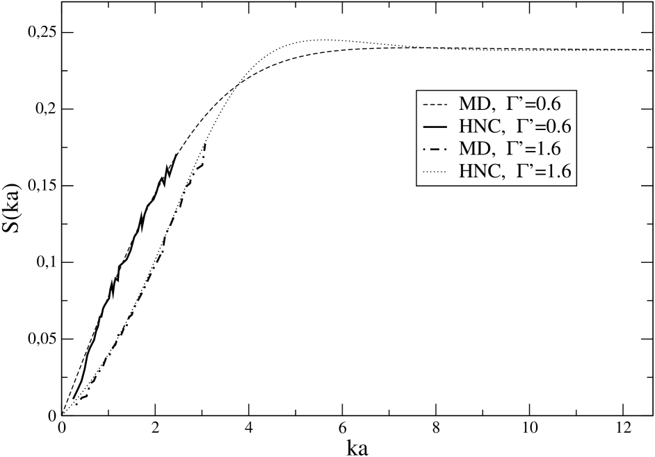
Figure 3: The PS of a $1/r^{2}$ OCP for two different values of the coupling parameter $\Gamma^{\prime}$. Excellent agreement is observed between the predictions from the HNC and MD in the range where they overlap. For the weak coupling case the HZ form for the PS $S(k)\propto k$ is clearly evident. The units are normalised to the ionic radius a. Note that the plot is on a linear-linear scale.

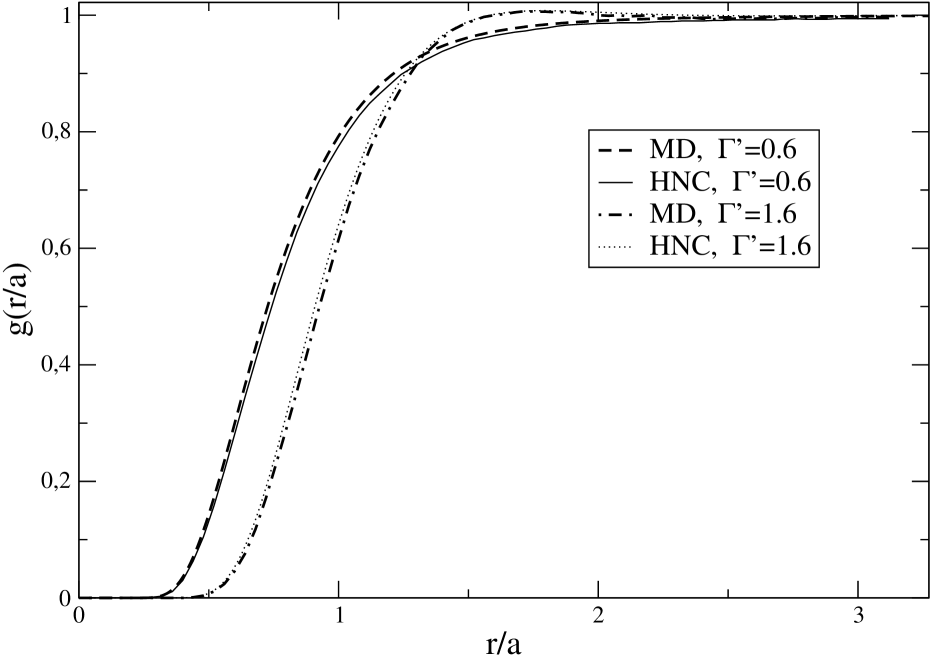
Figure 4: The correlation function in real space for the $1/r^{2}$ OCP for the same cases as in the previous figure. For the smaller coupling one has anti-correlation at all scales ($g(r)<1$) while for the larger coupling one sees, just as in the standard OCP, the correlation appear with the first neighbour (which becomes more localised as the temperature is lowered).

In the first subsection below we will present an example of a HZ spectrum generated with a simple $1/r^{2}$ potential. In the following subsection we present the method using the simplified PS of Eq.(58), while in the last subsection we give the potential which should allow the generation of the “realistic” cosmological PS of Eq.(57).

V.1 The HZ spectrum

We consider just the “primordial” part of the PS with the HZ behaviour $P(k)\sim k$. As mentioned in Sect. III, it has been shown in gjjlpsl02 by a simple screening argument that one expects to obtain such a PS at small $k$ in a modified OCP with interparticle potential $v(r)=1/r^{2}$. To verify this expectation we have used both the HNC and molecular dynamics as described above. In Fig. 3 the results for the PS are given for each case, and in Fig. 4 the correlation function in real space. Because the potential is still a pure power-law the phase space is, as for the standard OCP, one dimensional and may be characterised by a single dimensionless parameter analogous to that for the OCP. We make the obvious generalisation of the definition in Eq.(24):

$$\Gamma^{\prime}=\beta(Ze)^{2}/a^{2}.$$ (61)

The results from the HNC are valid in the infinit volume limit and show very good agreement with the prediction of the asymptotic form for both the PS and the correlation function given in gjjlpsl02 . The range of these behaviours is, as expected, greater for smaller values of the coupling, and the linearity of the PS in particular is clearly visible in this case. We have checked also that one recovers the characteristic behaviour of the correlation function at large scales $(g(r)-1)\sim-1/r^{4}$, which is also that of cosmological models with this PS (see gsljp-springer ; glass ).

The simulations of molecular dynamics were performed in the micro-canonical ensemble with the methods described in Sect. IV above, with N=4000 particles . This corresponds to a simulation box with side of length $L=\left(\frac{4\pi}{3}N\right)^{\frac{1}{3}}a\approx 25.6$. Over this limited range very good agreement is seen with the results from the HNC in all cases, with some remaining statistical fluctuations. The units of time used in the simulations is $\tau=\sqrt{3}\omega_{p}^{-1}$ with $\omega_{p}^{2}=4\pi n_{0}(Ze)^{2}/m$. To ensure good conservation of energy we have used a time increment of typically $\Delta t\sim 10^{-2}\tau$, which leads to fluctuations of $\sim 10^{-7}$ in the energy. The system evolves for $10^{5}\tau$ times steps, at which point it has reached thermal equilibrium. Then the PS and correlation functions are computed over many realizations of the system. By the ergodic principle this is equivalent to performing an ensemble average. Each realization is thus a configuration of the system at each time step. We compute the average in all the simulations over $50000$ time steps, which leaves only very small fluctuations about the average.

V.2 CDM-type spectra: simple model

Let us now consider the spectrum (58). We have seen that the small $k$ part of the spectrum can indeed be produced by a repulsive $1/r^{2}$ potential. We will now use the inversion of the HNC to determine the short range potential which needs to be added to produce the modification at larger $k$ described by Eq. (58).

This input continuous model PS contains four free parameters. We define $S(k)$, the PS of the discretisation, using Eq. (15) with $D(k)$ as in Eq. (59), and $k_{d}$ expressed in terms of $a$ by its bounding value in Eq. (60). In discretising we thus introduce just one independent length scale, fixed by the particle density $n_{0}$, and which we identify by convention with the ionic radius $a$ defined in Eq. (23). To fix the model being discretised we must specify $S(k)$ by giving the three dimensionful quantities (${\cal N}$, $A$ and $k_{c}$) in units of $a$. The parameter $\alpha$ in Eq. (58) fixes the slope of the power spectrum $P(k)\sim k^{1-\alpha}$ beyond the “turn-over” from the small $k$ behaviour $P(k)\sim k$. As discussed above relevant values are in the range $2<\alpha<4$, and we will consider here the case $\alpha=3$ (i.e. $P(k)\sim k^{-2}$ beyond the turn-over).

The cut-off parameter $k_{c}$ is required simply to make the theoretical one-point variance (given by the integral of the PS) finite. We will take it, however, to be much larger than $1/a$, so that it will play essentially no role in what follows other than to regularise Fourier transforms at small separations (e.g. in determining the theoretical correlation function $\xi_{c}(r)$ associated to Eq. (58)). The numerical results below used $k_{c}=2.7/a$.

We thus have essentially just the two parameters $A$ and ${\cal N}$ to specify in terms of $a$. The former fixes the scale of the maximum (or “turn-over) in the PS:

$$k_{t}\simeq\frac{1}{(\alpha-1)^{1/\alpha}}\frac{1}{A}\,.$$ (62)

When we simulate the molecular dynamics we have a finite box of side $L=\left(\frac{4\pi}{3}N\right)^{{1}/{3}}a$, and thus a finite range, from the inter-particle distance to the box size, in which we can attempt to represent the theoretical correlation properties. In $k$ space this is the range $k_{f}<k<k_{d}$, where $k_{f}=2\pi/L$ is the fundamental mode and $k_{d}$ the $k$-space scale beyond which $S(k)$ necessarily deviates from the input $P(k)$. We thus choose $A$ so that $k_{t}$ falls in this range. Once this choice is made ${\cal N}$ then fixes the overall normalisation. As discussed in Sect. II.4, the relevant dimensionless parameter to characterise the amplitude of the fluctuations is $n_{0}P(k_{d})$. The natural choice, which we will use, is $n_{0}P(k_{d})\approx 1$ i.e. the theoretical power is roughly at the Poisson level at the inverse of the interparticle distance.

We will consider here a simulation of $8788$ particles i.e. $L\approx 33.3a$ and $k_{f}\approx 0.19/a$. We choose $k_{t}=0.52/a$ so that we have a small range of wavenumbers in which the PS is linear in $k$ inside the box. For the chosen value of $\alpha=3$ this gives $A\approx 1.51a$. Finally we take ${\cal N}=30a^{4}$ which corresponds to $n_{0}P(k_{d})=0.47$. In Fig. 5 the pair $P(k)$ and $S(k)$ corresponding to these values are shown, and in Fig. 6 the corresponding correlation function pair $\xi_{c}(r)$ and $h(r)$.

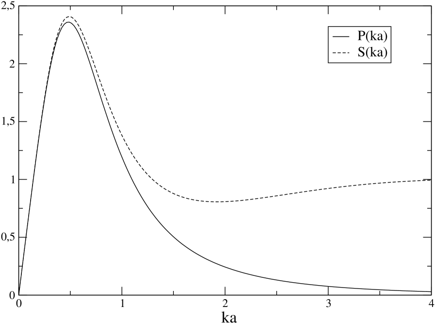
Figure 5: The theoretical PS $P(k)$ and its discretisation $S(k)$, for the parameters choices given in the text. They differ as described by the chosen smoothing function $D(k)$, for $ka\raise 1.72218pt\hbox{$>$}\kern-6.99997pt\lower 2.6694pt\hbox{$\sim$}1$, with $S(k)$ going asymptotically to $1/n_{0}$, where $n_{0}=3/(4\pi a^{3})$ is the particle density for the discretisation.

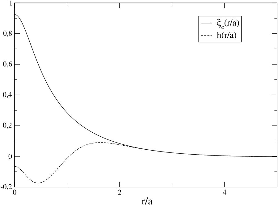
Figure 6: The theoretical input two-point correlation function $\xi_{c}(r)$ and that of the corresponding discretisation $h(r)$.

As discussed in Sect. II.2 the theoretical PS $P(k)$ can be interpreted as that of a continuous mass distribution obtained by a physical smoothing with a function, whose Fourier transform is given by

$$\lvert W_{k_{d},n_{0}}(k)\rvert^{-2}=1+\frac{\left(1+(Ak)^{\alpha}\right)(1-e^{-k^{2}/2k_{d}^{2}})}{n_{0}{\cal N}k}\exp(k/k_{c}).$$ (63)

The corresponding real space smoothing function, calculated numerically for our chosen $S(k)$, is shown in Fig. 7. It decays at large separation faster than $1/r^{4}$, and is thus a localised smoothing in the sense we discussed in Sect. II. It has, however, the rather unsatisfactory feature of oscillating through negative values, albeit when the amplitude is already very small. We could, in principle, remedy this by making a slightly different (but more complex) choice of $D(k)$, but we do not anticipate that it should cause any significant change in our results.

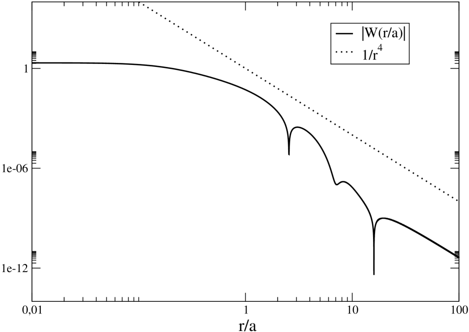
Figure 7: The window function in real space $\lvert W_{k_{d},n_{0}}(r)\rvert$.

Given our chosen $S(k)$ we can now use the inverted HNC equation Eq. (39) to determine the combination $\beta v(r)$. The results are shown in Fig. 8. For $r/a>5$ the potential approaches the $1/r^{2}$ form corresponding to the small $k$ behaviour of the PS. For $r\raise 1.72218pt\hbox{$>$}\kern-6.99997pt\lower 2.6694pt\hbox{$\sim$}4a$ the correlation function is negative (i.e. the system is anti-correlated) while it becomes positive for smaller scales. Correspondingly the potential becomes attractive at approximately this scale. At a smaller scale $r<lsim2a$, we see that the continuous correlation function $\xi_{c}(r)$ (i.e. the Fourier transform of Eq. (58)) begins to deviate from the two-point correlation function $h(r)$ of the discretisation.

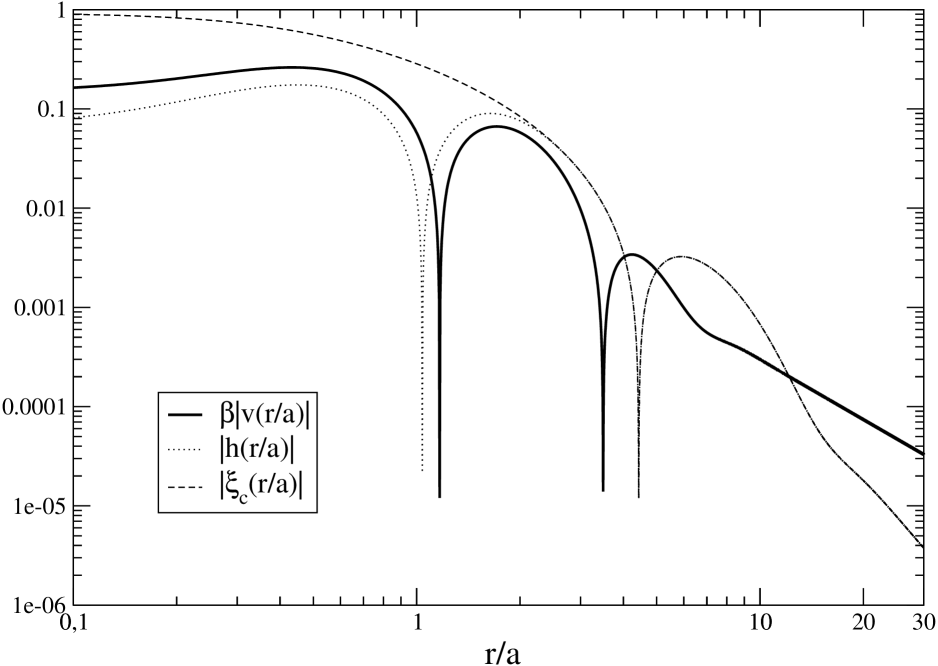
Figure 8: The correlation function, discretised correlation function, and interaction potential obtained by the inversion of the HNC for a PS as given in Eq.(58), with ${\cal N}=20\,a^{4}$, $A\approx 0.69\,a$ $k_{c}=2.7/a$ and $k_{d}=1.55/a$.

As anticipated, given the characteristics of $S(k)$ which describes a positively correlated system at small scales (associated with the negative power law behaviour for $k>k_{t}$), the potential $v(r)$ is attractive at small scales. Such a potential does not have a well defined thermal equilibrium ruelle . To define a system whose thermal equilibrium gives the desired $S(k)$, we therefore add a repulsive core at some scale. We take a core of the form $v_{c}(r)=0.2a^{10}/r^{12}$ (in units $Ze=1$) which has a negligible effect on the potential at and above the scale $a$. We check that this full potential, used in the direct HNC, indeed reproduces the input $S(k)$ to a very good approximation. This is also a good consistency check on the use of the HNC for the chosen parameter values, in particular the normalisation given by the chosen value of ${\cal N}$. If ${\cal N}$ were too large we would no longer be in the regime of weak correlations for which the HNC equation is valid.

We finally perform a simulation of molecular dynamics with the determined potential to obtain configurations of points with the PS desired. The HNC equation gives the potential times the temperature $\beta v(r)$, so we must choose a temperature. Any choice which keeps us in the regime of validity of the HNC should be appropriate. We make the simple choice $\beta=a^{2}$ (in units $Ze=1$ i.e. in which the large separation limit of the potential is always simply $v(r)=1/r^{2}$) which gives $\Gamma^{\prime}=1$ in Eq. (61) where, as we have discussed, the HNC gives very accurate results for the $1/r^{2}$ potential .

In the simulation we use this temperature to fix the initial velocities, taking them to be random, and Gaussian distributed, with the corresponding variance. Typically the system thermalises at a slightly different temperature (as there is also a change in potential energy relative to the initial configuration). By trial and error one can converge on the initial dispersion which gives the desired final temperature. For these simulations this involved typically a few trials. We will return to this point briefly in the final section below.

In Fig. 9 and Fig. 10 are shown the results for molecular dynamics simulations with the potential determined from the HNC as described above (and for a final temperature s.t. $\beta=1/a^{2}$).

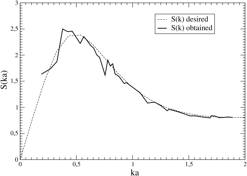
Figure 9: The PS measured in a simulation of the molecular dynamics of $8788$ particles for the potential shown in the previous figure. Also shown is the input PS i.e. the PS of a system at equilibrium with this potential as calculated in the HNC.

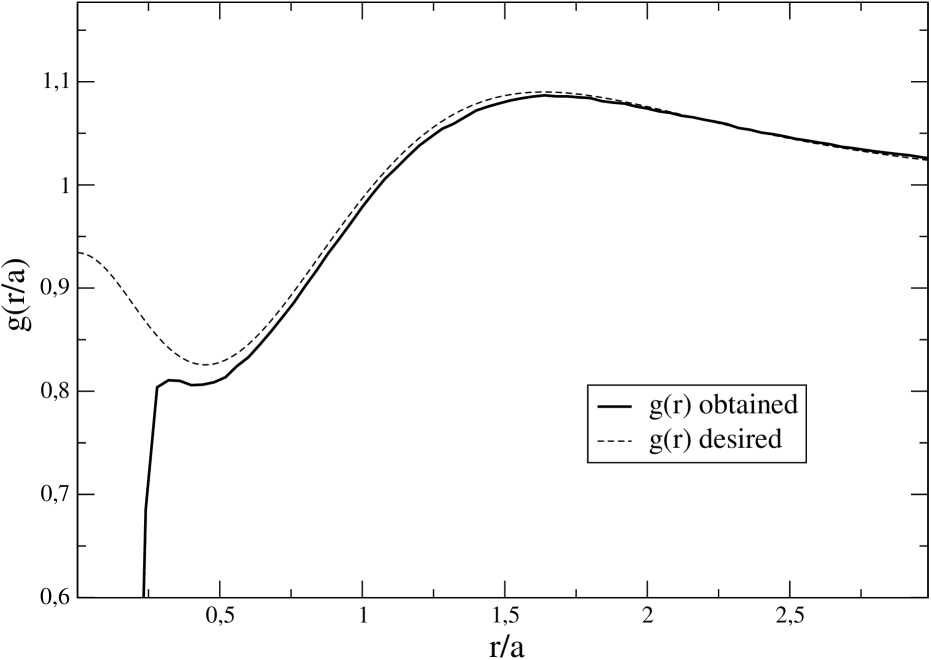
Figure 10: The real space correlation function for the same cases as in the previous figure. The abrupt break to anti-correlation at about $r/a\approx 0.25$ comes from the hard core introduced to ensure stability of the system.

The agreement is satisfactory, in the sense that we reproduce quite well the correlation properties of the discretisation we have defined, in both real and reciprocal space. The effect of the hard-core is visible in real space in the abrupt break in the correlation function, and it has a negligible effect above the scale $r\approx 0.2a$ below which it dominates .

V.3 CDM-type spectra: realistic model

We consider finally the determination of the potential which should reproduce the cosmological PS (57), with the parameters of a currently standard cosmological simulation (e.g. like that taken as initial condition in the simulations of the VIRGO consortium jenkins98 ). To do so we must choose, in units of physical length, the scale $a$ characterising the desired discretisation. For our example, we choose this scale by supposing we have the same physical density of point $n_{0}$ as in some typical simulations of the VIRGO consortium: we suppose that we have the particle density corresponding to $256^{3}$ particles in a cubic box of side $239.5\mathrm{h^{-1}Mpc}$. The gives $a\approx 0.58\mathrm{h^{-1}Mpc}$. We take our initial time to correspond to red-shift $z=50$, and fix the normalization of the model at this time by the prescription that, using the extrapolation of linear theory, one obtains today (at $z=0$) $\sigma_{8}=1$. This corresponds to a normalisation such that $\sigma_{8}=1/(z+1)=1/51$, and the normalization factor is then ${\cal{N}}=29381\mathrm{(h^{-1}Mpc)^{4}}$. The discretisation scale $k_{d}$ introduced is chosen again at the bounding value $k_{d}\approx 1.55/a$. In Fig. 11 are shown the correlation functions and the potential for this case. We note the same $1/r^{2}$ behaviour at large scales, but the potential is more complicated at small scales due to the oscillations in the direct correlation function $c(r)$. By simulating the molecular dynamics with this potential with a sufficiently large number of particles, as we have done for a smaller number of particles for the simpler cases, we should obtain a discretisation of the model with the properties Eqs. (21) and (22).

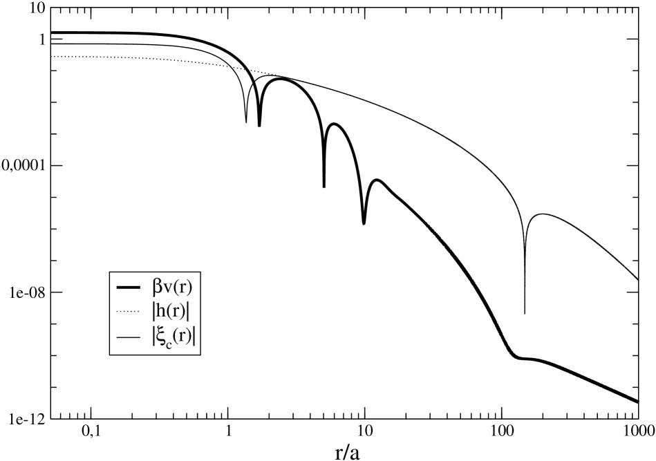
Figure 11: Correlation functions and interaction potential obtained for the cosmological CDM spectrum described in the text.

VI OTHER ISSUES AND CONCLUSIONS

We have presented a new method to generate discrete distributions with desired two-point correlation properties. It provides a promising alternative to the standard method for generating initial conditions for N-body simulation in cosmology used, which involves displacing particles in a prescribed manner of a perfect lattice (or, sometimes, “glassy” configuration). As discussed in detail in jm04 this latter method usually represents well the input theoretical PS in Fourier space at wave-numbers below the Nyquist frequency, but produces in real space a system with correlation properties which are a mixture of those of the initial unperturbed lattice configuration and those of the theoretical model. One obtains, in particular, a two-point correlation function which is a rapidly oscillating function up to very large separations, which is a behaviour completely different to that of the theoretical model. In comparison the interest of this new method is thus that it can give (by construction) a faithful representation of the two-point statistical properties of a CDM-like spectrum in both real and Fourier space. In particular, in the examples we have considered, the correlation function in real space converges very well to the theoretical input correlation function at a scale slightly larger than $a$. Increasing the number of particles for the same physical size of the system, the interparticle distance $a$, and thus this scale, diminishes. In Fourier space the agreement is good (by construction) for wavenumbers less than roughly a factor of two smaller than the inverse of the scale $a$.

In conclusion we now discuss the remaining steps which are required to apply the method fully in the context of cosmological simulations. Specifically we address the question of the generation of initial velocities required for such simulations, and then that of the modifications necessary to produce much larger distributions than those described here. Before doing so we first summarise briefly the method.

VI.1 Summary of the method

The principal steps involved in going from an initial input theoretical PS P(k) to an output configuration of initial conditions are the following :

• 1. Determination of the function $S(k)$, the PS of the discretisation of $P(k)$ which we wish to generate. As discussed in Sect. II this choice is necessary as the PS of the point distribution cannot be equal to $P(k)$, because continuous and discrete PS have intrinsically different asymptotic properties at large $k$. The relation between the two is given by Eq. (15), which, requires the choice of a smoothing function $D(k)$. We have considered the simple choice $D(k)=1-e^{-k^{2}/2k_{d}^{2}}$, and have taken $k_{d}$ as given by its upper bound as in Eq. (60). The passage from $P(k)$ to its discretisation $S(k)$ involves therefore the introduction of only one parameter, a length scale which we have chosen to take as $a$, determined by the particle density $n_{0}$ through Eq. (23).

• 2. Choice of parameter values in S(k). Given the functional form of $S(k)$ one must give the specific model by choosing the values of the parameters. This means simply that the length scale $a$ must be associated to a physical scale of the model (or, equivalently, that the dimensionful parameters in $P(k)$ be specified in units of $a$). In making this choice of parameters there are two essential points. Firstly, the system will be simulated with a finite number of particles $N$, and thus a finite box (of side $L=\left(\frac{4\pi}{3}N\right)^{\frac{1}{3}}a$). The parameters choices should evidently mean that the important characteristic scales in $P(k)$ fall well inside the range $k_{f}<k<k_{d}$ (where $k_{f}$ is the fundamental mode of the box). Secondly the overall amplitude of $P(k)$ should be specified by a choice of the dimensionless parameter $n_{0}P(k_{d})$, and should make this parameter of order unity.

• 3. Determination of the two-body potential. Given a specific $S(k)$ the inversion procedure using the HNC, described in detail in Section III, is used to determine $\beta v(r)$ (where $v(r)$ is the two-body interaction potential). If this associated potential does not give a stable thermal equilibrium, a hard core is added well below the scale $a$ to ensure stability. Using this full potential (i.e. obtained by adding the core) one verifies that the direct HNC give the desired $S(k)$. This is also a check on the applicability of the HNC at the chosen amplitude.

• 4. Generation of realizations of the discretisation. The molecular dynamics of $N$ particles interacting with the potential $v(r)$ is simulated, starting from initial velocities corresponding to a chosen temperature. A simple appropriate choice of the latter is $\beta=1/a^{2}$ (in units in which the long-range part of the potential is $v(r)=1/r^{2}$). If the system thermalises at a slightly different temperature, the initial velocities can be appropriately modified by trial and error.

VI.2 Generation of initial velocities

In the initial conditions of cosmological simulations of gravity, velocities must evidently also be ascribed to the particles of the distribution. We will now explain that these velocites can be generated for our point distributions using the same method as in the standard algorithm.

In cosmological models small initial density perturbations evolve, in linear theory, as a combination of a growing and a decaying mode. The choice of velocities which is almost always appropriate corresponds to the selection of only the growing mode. In practice this is implemented using the Zeldovich approximation zel ; buchert , which gives the motion of a fluid element in a self-gravitating fluid as

$${\vec{x}}({\vec{q}},t)={\vec{q}}+f(t){\vec{u}}({\vec{q}})$$ (64)

where ${\vec{x}}$ is the (Eulerian) position of the fluid element, ${\vec{q}}$ its Lagrangian coordinate and $f(t)$ is a function of (cosmic) time $t$. In an expanding universe ${\vec{x}}$ is the comoving coordinate of the fluid element, related to its physical coordinate ${\vec{r}}$ by ${\vec{r}}=a(t){\vec{x}}$. We will suppose that ${\vec{q}}$ is the (comoving) position of the fluid element at a time $t_{0}$ i.e. $f(t_{0})=0$.

Using Eq. (64) in the continuity equation, expanded to linear order in the displacement field ${\vec{u}}$, gives

$$\rho(\vec{x},t)=\rho(\vec{q})\left[1-f(t){\vec{\nabla}}_{q}\cdot{\vec{u}}\right]\,.$$ (65)

where $\rho(\vec{x},t)$ and $\rho(\vec{q})$ are the mass densities in Eulerian and Lagrangian coordinates respectively. The peculiar gravitational field, defined by ${\vec{g}}=\ddot{\vec{r}}-\frac{\ddot{a}}{a}{\vec{r}}$ obeys the Poisson-type equation

$${\vec{\nabla}}_{r}\cdot{\vec{g}}=-4\pi G\left(\rho({\vec{r}},t)-\frac{\rho_{0}}{a^{3}}\right)$$ (66)

sourced by the density fluctuations in matter about the mean density ($\rho_{0}$ is the constant mean comoving matter density of the universe, equal to the mean density in physical coordinates when $a=1$), and is given, using Eq. (64), by

$${\vec{g}}=a(t)[\ddot{f}(t)+2H(t)\dot{f}(t)]{\vec{u}}({\vec{q}})$$ (67)

where $H(t)=\dot{a}/a$. Substituting this relation in Eq. (66) at $t=t_{0}$ (when $\vec{x}=\vec{q}$), and then in Eq. (65), it is easy to verify that, to linear order in the density perturbations about the mean comoving density $\rho_{0}$,

$$\frac{\rho(\vec{x},t)-\rho_{0}}{\rho_{0}}=\left[1+\frac{4\pi G\rho_{0}f(t)}{\ddot{f}(t_{0})+2H(t_{0})\dot{f}(t_{0})}\right]\frac{\rho(\vec{q})-\rho_{0}}{\rho_{0}}$$ (68)

where we have chosen $a(t_{0})=1$.

The evolution, on the other hand, of density fluctuations in Eulerian linear theory is given by

$$\frac{\rho(\vec{x},t)-\rho_{0}}{\rho_{0}}=D(t)\frac{\rho(\vec{q})-\rho_{0}}{\rho_{0}}$$ (69)

where $D(t)$ is a solution of

$${\ddot{D}(t)+2H\dot{D}(t)}-\frac{4\pi G\rho_{0}}{a^{3}}D(t)=0\,,$$ (70)

normalised to $D(t_{0})=1$. Thus taking $f(t)=D(t)-D(t_{0})$ in Eq. (68), one obtains Eq. (69) i.e. from Eq. (64) with $f(t)=D(t)-D(t_{0})$ one recovers Eulerian linear theory for the evolution of small amplitude density fluctuations. In particular choosing the growing mode solution (i.e. $D_{+}(t)=(t/t_{0})^{\frac{2}{3}}$ for a flat matter dominated cosmology) gives fluctuations evolving in the pure growing mode as usually desired.

Using Eq. (64) the physical velocity of a fluid element is $\dot{\vec{r}}=H{\vec{r}}+{\vec{v}}$, where

$${\vec{v}}=a(t)\dot{f}(t){\vec{u}}({\vec{q}})$$ (71)

is its peculiar velocity. Now through Eq. (67) it follows that

$${\vec{v}}=\frac{\dot{f}(t)}{\ddot{f}(t)+2H(t)\dot{f}(t)}\,{\vec{g}}\,.$$ (72)

To fix the initial velocities in our case we therefore simply use the Zeldovich approximation as given by Eq. (64), the ${\vec{q}}$ being identified with the initial positions of our particles in the initial configuration corresponding to the required initial time $t_{0}$. Eq. (72) evaluated at $t=t_{0}$ and with $f(t)=D_{+}(t)$ specifies the velocities, in terms of the peculiar gravitational field ${\vec{g}}$ at each point in the initial configuration.

It is perhaps useful to clarify the relation of this use of the Zeldovich approximation to the usual one in setting up initial conditions for cosmological NBS. To do so we write Eq. (64) as

$${\vec{x}}({\vec{R}},t)={\vec{R}}+D_{+}(t){\vec{u}}({\vec{R}})$$ (73)

by a change of the Lagrangian variable ${\vec{R}}={\vec{q}}-{\vec{u}}({\vec{q}})$ buchert . One has $D_{+}(t\rightarrow 0)=0$ so that the density in the coordinates ${\vec{R}}$ is that of the universe as $t\rightarrow 0$. In the standard method of setting up initial conditions in cosmological simulations, these initial positions ${\vec{R}}$ are taken to be those of points in a “uniform” configuration: usually a lattice, or sometimes also a “glassy” configuration white . The initial conditions (at $t=t_{0}$) are then generated by moving the points to ${\vec{q}}={\vec{R}}+{\vec{u}}({\vec{R}})$ with the displacements ${\vec{u}}({\vec{R}})$ given through Eq. (67), the gravitational field being evaluated at the position ${\vec{R}}$ by a realization of the desired gravitational potential field (which in turn is determined by the theoretical power spectrum through the Poisson equation). This is accurate to linear order in the displacement field.

The crucial point which allows us to use the Zeldovich approximation is that this approximation does not require, as is supposed in its usage just described in the standard algorithm for generating initial conditions, that the evolution of the fluid start from a perfectly homogeneous configuration. Indeed the Zeldovich approximation is simply an asymptotic solution of the evolution of a self-gravitating fluid away from a generic initial configuration with some initial velocity and gravitational field buchert . More specifically all that is required to recover the linear amplification of density fluctuations which follow from the Zeldovich approximation, as described in the first part of this section, is that the density fluctuations are small. In this respect, we note that one can actually consider the standard algorithm as a two step process in complete analogy to our method. In the first step particles are displaced off a lattice (or other “uniform” particle configuration) in order to produce a distribution with a power spectrum resembling as closely as possible that of the theoretical power spectrum $P(k)$. This does not in fact require the use of the Zeldovich approximation, but only the continuity equation. Indeed from Eq. (73) with $D(t_{0})=1$, and assuming $\rho(\vec{R})=\rho_{0}$, the continuity equation gives

$$\frac{\rho(\vec{x},t)-\rho_{0}}{\rho_{0}}=-{\vec{\nabla}}_{R}\cdot{\vec{u}}({\vec{R}})\,.$$ (74)

From this it follows that it is sufficient to take ${\vec{u}}({\vec{R}})$ to be the gradient of a scalar field $\phi(\vec{R})$ (as any rotational component for ${\vec{u}}$ will not generate density fluctuations). Through Eq. (74) we have that $|\tilde{\phi}(\vec{k})|^{2}=P(k)/k^{4}$, and thus that $\phi(\vec{R})$ is just proportional to the gravitational potential. The procedure is thus precisely the standard one. The second step then consists in generating the velocities, and one can proceed exactly as we have described for our method, using now explicitly the Zeldovich approximation and, specifically, Eq. (72) with the gravitational field ${\vec{g}}$ given at each point in the perturbed configuration (i.e. at the Lagrangian coordinate $\vec{q}$). To the linear order in the displacements this is identical to the standard prescription.

VI.3 Generation of larger distributions

To test the proposed method here we have generated particle distributions with at most of order ten thousand particles, a number typical in statistical physics for the simulation of the molecular dynamics of systems of the type we have used (and for which the numerical codes have been conceived). It may be interesting and useful to evolve configurations of this size generated in this way, and by the standard method, under their self-gravity and to do a comparative study of this evolution. However, to use it as a truly alternative method in full cosmological simulations, it will be necessary to generate much larger configurations: in this context simulations typically now involve, at a minimum, hundreds of thousands of particles.

The Ewald summation method we have used here can be shown perram-scaling-ewald to scale (for a fixed precision on the calculation of the energy and forces) as $N^{3/2}$. Given that the largest simulations we have reported here, of approximately nine thousand particles, ran in about one day on a typical current PC, we could simulate only a slightly larger number in a reasonable time with our code. There are, however, well documented ways of speeding up the Ewald sum method by calculating the reciprocal space part of the sum on a grid. One can then employ rapid FFT algorithms, which scale as $N\log N$ Ewald-FFT , with the direct space part of the sum scaling as $N$. There are numerous variants (e.g. P3M, PME, SPME), which differ primarily in how the charges (or masses) are assigned to the grid. Going beyond the Ewald method, or in combination with it, an even faster algorithm is the Fast Multipole Method (FMM) (see e.g. multi-pole methods ). It is based on a decomposition of the system into sub-volumes, with the interaction between the charges contained in a given volume with those in a sufficiently distant sub-volume being calculated with a multipole expansion. Most of these techniques are of course known in the context of cosmological NBS (e.g. EDFW , couchman ) where they have been applied to gravity. Note, however, that their use if not limited to this case, and in particular does not require that the potential necessarily obey a local equation like the Poisson equation as for the $1/r$ potential.

VI.4 Other remarks

Another possible improvement concerns the choice of initial velocities in our simulations of the molecular dynamics. When introducing the potential calculated with HNC we implictly choose the equilibrium temperature before performing the MD simulation. Thus, as explained above, we put the initial velocities to get the chosen final temperature. The problem is that we do not know a priori how the system is going to reach equilibrium and it is necessary to do trials with different initial velocities until the desired equilibrium temperature is attained. A solution to this problem would be to modify the MD to work in the canonical ensemble (in which the temperature is fixed) rather than in the micro-canonical ensemble as we have done here.

We remark finally that we have not attempted here to address at all the very interesting underlying question motivating this work of the importance of the accuracy and nature of the discrete representations of cosmological IC in the dynamical evolution under gravity of these IC. Our purpose here has been to provide an alternative method for representing IC which should allow such questions to be addressed with a new method, and hopefully answered, in due course.

We thank J.M. Caillol, A. Gabrielli and F. Sylos Labini for useful discussions and comments.

References

- (1) G. Efstathiou, M. Davis, C. Frenk and S. White, Astrophys.J. Supp. 57, 241 (1985).
- (2) S.D.M. White, Lectures given at Les Houches astro-ph/9410043 (1993).
-
(3)
H.M.P. Couchman, “Cosmological simulations using
particle mesh methods”,
http://www-hpcc.astro.washington.edu/Simulations/
DARK_MATTER/adapintro.html - (4) Ya.B. Zeldovich, Astron.& Astrophys. 5, 84-89(1970).
- (5) T. Buchert, Mon. Not. R. Ast. Soc, 254, 729-737,(1992).
- (6) T. Baertschiger and F. Sylos Labini, Europhys Lett., 57, 322 (2002).
- (7) A. Knebe and A. Domínguez, Europhys Lett., 63, 631 (2002).
- (8) A. Knebe and A. Domínguez, Publ. Astron. Soc. Pac. 20, 1, (2003).
- (9) A. Jenkins et al., Astrophys. J. 499 (1998) 20.
- (10) M.Joyce and B. Marcos, astro-ph/0410451.
- (11) A. Gabrielli, B. Jancovici, M. Joyce, J.L. Lebowitz, L. Pietronero and F. Sylos Labini, Phys. Rev. D, D67 (2003) 043506.
- (12) P. J. E. Peebles, The Large-Scale Structure of the Universe (Princeton University Press, NJ, 1980).
- (13) A. Gabrielli, F. Sylos Labini, M. Joyce & L. Pietronero, Statistical Physics for Cosmic Structure, Springer Verlag, Berlin (2004), in press.
- (14) A. Gabrielli, M. Joyce and F. Sylos Labini, Phys. Rev. D 65 (2002) 083523.
- (15) A. Gabrielli, Phys. Rev. E, to appear; cond-mat/0409594.
- (16) M. Baus and J.-P. Hansen, Phys. Rept. 59 (1980) 1.
- (17) G. S. Stringfellow, H. E. DeWitt, and W. L. Slattery Phys. Rev. A 41, 1105 (1990)
- (18) J. Beck, Acta Mathematica 159, 1-878282 (1987).
- (19) J.-P. Hansen and I. McDonald, Theory of Simple Liquids, Academic Press, London, 1976.
- (20) M. Wu, cond-mat/0112138v1.
- (21) G. Salin and J.-M. Caillol, J. Chem. Phys. 113 (2000) 10459.
- (22) D. Ruelle, Statistical Mechanics, Benjamin (1969).
- (23) V. Krakoviack, J.-P. Hansen and A.A. Louis, Phys. Rev. E 67, 041801 (2003).
- (24) J.W. Perram, H.G. Petersen and S.W. de Leeuw, Mol. Phys. 65, 875 (1988).
- (25) See, for example, A.Y. Toukmaji et al, J. Chem. Phys. 113, 10913 (2000); C. Sagui, J. Chem. Phys. 114, 6578 (2001); Essmann et al, J. Chem. Phys. 103, 8577 (1995)
- (26) Z.H. Duan et al., J. Chem. Phys. 113, 3492 (2000)