Can we test Dark Energy with Running Fundamental Constants ?

Abstract

We investigate a link between the running of the fine structure constant $\alpha$ and a time evolving scalar dark energy field. Employing a versatile parameterization for the equation of state, we exhaustively cover the space of dark energy models. Under the assumption that the change in $\alpha$ is to first order given by the evolution of the Quintessence field, we show that current Oklo, Quasi Stellar Objects and Equivalence Principle observations restrict the model parameters considerably stronger than observations of the Cosmic Microwave Background, Large Scale Structure and Supernovae Ia combined.

Observations of Supernovae Ia (SNe Ia) Riess:2004nr , the Cosmic Microwave Background (CMB) Spergel:2003cb ; Readhead:2004gy ; Goldstein:2002gf ; Rebolo:2004vp and Large Scale Structure (LSS) Tegmark:2003ud ; Hawkins:2002sg all point towards some form of dark energy. Over the years, theorists have come up with various models to explain the nature of dark energy Wetterich:fm ; Ratra:1987rm ; Caldwell:1997ii ; Caldwell:1999ew ; Freese:2002sq ; Bento:2002ps ; Bousso:2000xa (to name a few). In particular, it seems plausible that dark energy may be described by an (effective Kolda:1999wq ; Peccei:2000rz ; Doran:2002bc ; Carroll:2003st ) scalar field. Provided no symmetry cancels it, there will be a term in the effective Lagrangian coupling baryonic matter to the scalar field. If this field evolved over cosmological times, such a coupling would lead to a time dependence of the coupling “constants” of baryonic matter Wetterich:1987fk ; Sandvik:2001rv ; Damour:2002nv ; Wetterich:2002wm ; Wetterich:2003jt . Indeed, bounds on the time variation of these “constants” restrict the evolution of the scalar field and the strength of this coupling Wetterich:1987fk .

Since the days of Dirac Dirac:1937ti , it has been speculated that the fundamental constants of nature may vary. In a realistic GUT scenario, the variation of different couplings is interconnected Langacker:2001td ; Calmet:2001nu ; Mueller:2004gu . We will ignore this interdependence in the following and concentrate on a change in the fine structure constant $\alpha$ with all other “constants” fixed. Lacking detailed knowledge of the dependence of $\alpha$ on the scalar field, we make the Ansatz

$$\alpha(\varphi)=\alpha_{0}+\alpha_{0}\left(\frac{\partial\ln\alpha}{\partial\varphi}\right)_{|\varphi=\varphi_{0}}\left[\varphi(z)-\varphi_{0}\right].$$ (1)

Thus, fixing the Taylor coefficient $\partial\ln\alpha/\partial\varphi$ determines the evolution of $\alpha$ as a function of $\varphi$. This has immediate consequences: if the fine structure was indeed different at higher redshifts, the scalar field must have evolved since then. Yet, the Oklo nuclear reactor strongly limits the change of $\alpha$ at low redshifts $z\approx 0.1$. In our Ansatz, freezing $\alpha$ is equivalent to slowing down the evolution of $\varphi$. As the kinetic energy (of a canonical scalar field) is given by $T=\frac{1}{2}a^{-2}\dot{\bar{\varphi}}^{2}$, this leads to a drop in $T$ and therefore to an equation of state $w$ that approaches that of a cosmological constant

$$w=\frac{T-V}{T+V}\to-1.$$ (2)

In such a scenario, the equation of state of the scalar field crosses over from a more positive value at earlier times to a behavior that today mimics a cosmological constant Hebecker:2000zb ; Caldwell:2003vp ; Jassal:2004ej .

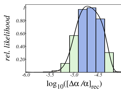
Figure 1: Marginalized likelihood distribution for the relative change of the fine structure constant quoted as $\log_{10}(\Delta\alpha_{\rm rec}/\alpha)$, so that $\Delta\alpha_{\rm rec}/\alpha=-10^{\log_{10}\left(\Delta\alpha_{\rm rec}/\alpha\right)}$. The distribution is obtained from Set I, i.e. Equivalence Principle, Oklo and QSO observations which are all at considerably lower redshifts than recombination. The dark shaded (blue), moderately shaded (green) and light (red) rectangles correspond to one, two and three $\sigma$ confidence regions. The distribution peaks at $-4.7$ and has width $+0.36,-0.26$. Thus the relative change of $\alpha$ at recombination is $\Delta\alpha_{\rm rec}/\alpha=-2^{+0.9}_{-2.3}\times 10^{-5}$.

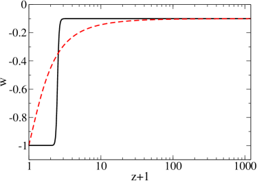
Figure 2: Equation of state for two different parameter sets of Equation (3) versus redshift. The equation of state in the early Universe is given by $w_{m}$ (here it is set to $-0.1$), while the one today is given by $w_{0}$ (here $-0.99$). The scale factor of the cross-over is determined by $a_{c}$ ($0.3$ for the solid curve, $0.7$ for the dashed curve), while the width of the transition is adjusted by $\Delta$ ($0.01$ for the solid curve, $0.1$ for the dashed one).

In order to describe such models, we employ the parameterization of Corasaniti:2002vg

$$w(a)=w_{0}+(w_{m}-w_{0})\times\frac{1+\exp(a_{c}/\Delta)}{1+\exp([a_{c}-a]/\Delta)}\\ \times\frac{1-\exp([1-a]/\Delta)}{1-\exp(1/\Delta)}.$$ (3)

This versatile parameterization is characterized by the equation of state of dark energy today $w_{0}$, the dark energy equation of state during earlier epochs $w_{m}$, a cross-over scale factor $a_{c}$ and a parameter $\Delta$ controlling the rapidity of this cross-over (see also Figure 2 for illustration). It has been shown (and we will confirm this later) that some of the four parameters $w_{0},\ w_{m},a_{c},\ \Delta$ are not too well constrained by present SNe Ia, CMB and LSS data Corasaniti:2004sz .

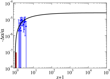
Figure 3: Minus the relative change of the fine structure constant $\Delta\alpha(z)/\alpha_{0}=\left[\alpha(z)-\alpha_{0}\right]/\alpha_{0}$ vs. redshift quoted as $z+1$. The QSO data is depicted at redshifts $z\sim 2-3$. In addition, we indicate the bound from the Oklo natural reactor $\Delta\alpha(z\approx 0.13)/\alpha_{0}>-9\times 10^{-8}$ by a slim vertical box in the lower left corner. The solid black curve is a model we picked at random from the Monte Carlo and which has parameters $\Omega_{m}h^{2}=0.12$, $h=0.55$,$\ w_{0}=-0.95$,$\ w_{m}=-0.26$, $\ a_{c}=0.8$, $\log_{10}(\Delta)=-2.8$ and $\Delta\alpha_{\rm rec}/\alpha=-2.4\times 10^{-5}$. Please note the moderate running of $\alpha$ at early times which is a direct result of the scalar field dynamics: with $w_{m}=0$, one gets $\varphi\propto\ln(1+z)$ and hence a moderate evolution at high redshifts. For $w_{m}<0$, the running is suppressed further as the total energy and hence the available kinetic energy of dark energy is considerably lower than for $w_{m}=0$. Hence, the change of $\alpha$ at nucleosynthesis would have negligible effect Mueller:2004gu .

In principle, a change of $\alpha$ at high redshifts will alter recombination. This effect has been discussed in Hannestad:1998xp ; Kaplinghat:1998ry ; Huey:2001ku and we have modified the recfast Seager:1999bc implementation of Cmbeasy Doran:2003sy to accommodate this deviation from standard recombination. Our results agree well with those of Kaplinghat:1998ry ; Sandvik:priv . However, we will soon see that Oklo and Quasi Stellar Objects (QSO) observations when explained in our framework limit the relative change of $\alpha$ at and during recombination. We will in the following quote this change at the pivotal redshift $z_{\rm rec}=1100$. Typically, in our scenario $\Delta\alpha_{\rm rec}/\alpha\equiv\left[\alpha(z_{\rm rec})-\alpha_{0}\right]/\alpha_{0}<10^{-4}$ (see also Figure 3). For such minute changes in $\alpha$, the recombination history remains practically unaltered. Therefore, considerations like that of Huey:2001ku ; Rocha:2003gc have negligible effect. This fact allows us to split the analysis in two parts (Set I and Set II): Set I with Equivalence principle, Oklo and QSO observations for which we do not need to include cosmological perturbations. Set II with WMAP, ACBAR, CBI, VSA, SDSS and SNe Ia Spergel:2003cb ; Readhead:2004gy ; Goldstein:2002gf ; Rebolo:2004vp ; Tegmark:2003ud ; Riess:2004nr observations (and hence cosmological perturbations), but constant $\alpha=\alpha_{0}$. In both cases, we employed the Markov Chain Monte Carlo (MCMC) Lewis:2002ah from the AnalyzeThis package Doran:2003ua of Cmbeasy Doran:2003sy .

For completeness, let us describe the well known reconstruction of the scalar field evolution from some parameterization $w(a)$: the starting point is a reconstruction of $\rho_{de}(a)$ by integrating $\textrm{d}\ln\rho_{de}=-3[1+w(a)]\textrm{d}\ln a$. This fixes $\dot{\varphi}(a)$, because $T=\frac{1}{2}(1+w)\rho_{de}=\frac{1}{2}a^{-2}\dot{\varphi}^{2}$. From this, $\varphi(a)$ simply follows by integrating $\dot{\varphi}$, where we use an integration constant to fix $\varphi_{0}=0$ for convenience. Demanding that $\alpha$ should change by $\Delta\alpha_{\rm rec}/\alpha$ at $z_{\rm rec}=1100$ and using $\varphi_{0}=0$, we can re-write Equation (1) as

$$\alpha(z)=\alpha_{0}+\alpha_{0}\left(\frac{\Delta\alpha_{\rm rec}}{\alpha}\right)\frac{\varphi(z)}{\varphi_{\rm rec}}.$$ (4)

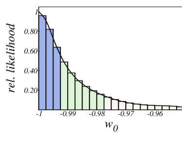
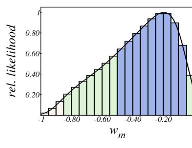
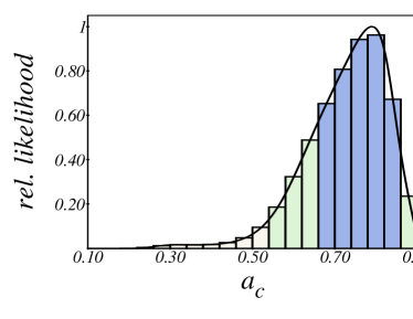
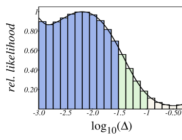
Figure 4: Marginalized likelihood distribution from the combination of Set I and Set II. The dark shaded (blue), moderately shaded (green) and light (red) rectangles correspond to one, two and three $\sigma$ confidence regions. At $2\sigma$ confidence level, we get $w_{0}<-0.97$ and $\Delta<0.1$, while with $1\sigma$ error bars, we have $w_{m}=-0.2^{+0.13}_{-0.30}$ and $a_{c}=0.79^{+0.06}_{-0.12}$.

For Set I, the parameters of the model were $\Omega_{m}h^{2}$,$\ h$,$\ w_{0},\ w_{m}$,$\ a_{c}$,$\ \log_{10}(\Delta)$ and $\log_{10}\left(\Delta\alpha_{\rm rec}/\alpha\right)$. Please note that we omit the spectral index $n$, optical depth $\tau$ and baryon fraction $\Omega_{b}h^{2}$ which are present in the Set II-analysis, because Set I data does not contain information on these parameters. Thus, the distribution in $n$,$\ \tau$ and $\Omega_{b}h^{2}$ is flat and our simulation for Set I can be thought of as trivially marginalized over $n$,$\ \tau$ and $\Omega_{b}h^{2}$. The Equivalence Principle is tested via the differential acceleration $\eta$ between test particles of equal mass but different composition Wetterich:2003jt

$$\eta=-3\times 1.75\cdot 10^{-2}\left(\frac{\partial\ln\alpha}{\partial\varphi}\right)_{\varphi=\varphi_{0}}^{2}\Delta R(1+Q).$$ (5)

Here, $\Delta R\equiv\Delta Z/(Z+N)\approx 0.1$ is the difference in composition and the factor $(1+Q)$ encodes the theoretical uncertainty in calculating $\eta$. As the true underlying theory is unknown, we ’guesstimate’ conservatively $(1+Q)\in[10^{-2},10^{2}]$ which is used as a flat prior. As current experiments give a null result baessler

$$\eta=0\pm 3\times 10^{-13},$$ (6)

$(1+Q)=10^{-2}$ (i.e. the lower bound) always agrees best with observations.

Roughly $1.8$ billion years ago (i.e. $z\approx 0.1$), the Oklo natural reactor was up and running. Until recently, the reactor was seen as providing yet another null result, namely Damour:1996zw

$$\frac{\Delta\alpha}{\alpha}_{\rm Oklo}=0^{+12}_{-9}\times 10^{-8}.$$ (7)

Yet, the latest calculation Lamoreaux:2003ii yields a positive detection of

$$\frac{\Delta\alpha}{\alpha}_{\rm Oklo}=45^{+7}_{-15}\times 10^{-8}$$ (8)

To complicate matters further Martins:2004ni , Fujii et. al Fujii:2003gu find two values,

$$\frac{\Delta\alpha}{\alpha}_{\rm Oklo} = (-0.8\pm 1.0)\times 10^{-8},$$ (9)

$$\frac{\Delta\alpha}{\alpha}_{\rm Oklo} = (8.8\pm 0.7)\times 10^{-8}.$$ (10)

We will take a conservative stand here (given the scatter in the calculations) and use the null-result of Damour:1996zw , Equation (7).

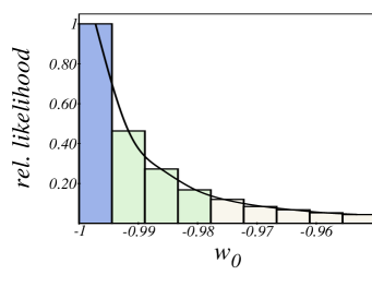
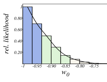
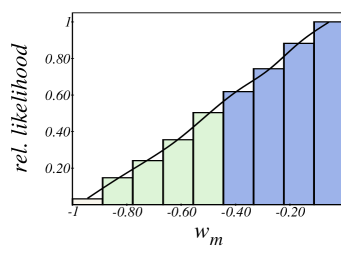
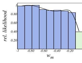
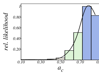
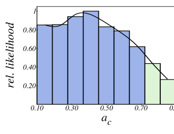
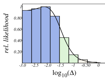
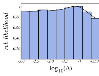
Figure 5: Marginalized likelihood distribution for the parameters of Equation (3). The left column derives from Oklo, QSO and Equivalence Principle observations, while the right column uses WMAP, ACBAR, CBI, VSA, SDSS and SNe Ia data. Please note that the bound on all parameters on the left is considerably tighter than that in the right column. The dark shaded (blue), moderately shaded (green) and light (red) rectangles correspond to one, two and three $\sigma$ confidence regions.

For QSO observations, we use the sample of Murphy:2003hw ; Murphy:priv which roughly translates into

$$\frac{\Delta\alpha}{\alpha}_{\rm QSO}=(-5\pm 1)\times 10^{-6}.$$ (11)

There have been contradicting claims about such QSO results Chand:2004ct . While time may tell what $\alpha$ really was at $z\approx 2$, we stick with Equation (11) for the purpose of this letter. So we ask: if $\alpha$ really changed in the past, what does it tell us about dark energy?

The main results of our Set I analysis are summarized in Figure 1 and the left column of Figure 5. From Figure 1, we see that $\Delta\alpha_{\rm rec}/\alpha=-2^{+0.9}_{-2.3}\times 10^{-5}$. Likewise, in the left column of Figure 5, we see that these measurements lead to strong bounds on the equation of state today. At $2\sigma$ confidence level, $w_{0}<-0.97$. In addition, the transition is restricted to occur rather swiftly (as seen from $\log_{10}(\Delta)$) and at rather recent times (as seen from $a_{c}$).

Turning to our Set II  analysis, the parameters were the amount of matter and baryons $\Omega_{m}h^{2}$ and $\Omega_{b}h^{2}$, Hubble constant $h$, optical depth to re-ionization $\tau$ and spectral index $n$ plus four parameters $w_{0}$,$\ w_{m}$,$\ a_{c}$,$\ \log_{10}(\Delta)$ of the dark energy model. As said, we did not need to take a varying $\alpha$ into account, because the allowed values of $\Delta\alpha_{\rm rec}/\alpha$ from Set I are minute in our framework and will not alter standard recombination. To test this model, we compared to WMAP, VSA, ACBAR, CBI, SDSS and SNe Ia measurements Spergel:2003cb ; Readhead:2004gy ; Goldstein:2002gf ; Rebolo:2004vp ; Tegmark:2003ud ; Riess:2004nr . The versatile (and therefore difficult to constrain) parameterization of Equation (3) has been under investigation in Corasaniti:2004sz . Our results agree well with those presented in that paper (compare the right column of our Figure 5 to Figure 6 of Corasaniti:2004sz ). With the exception of $w_{0}$, the constraints are considerably less tight than those inferred from the fine structure data. Combining Set I with Set II leads to the likelihood distributions shown in Figure 4 and represent our main results. At $2\sigma$ confidence level, we get $w_{0}<-0.97$ and $\Delta<0.1$. Quoting the $1\sigma$ error bars, we get $w_{m}=-0.2^{+0.13}_{-0.30}$ and $a_{c}=0.79^{+0.06}_{-0.12}$.

In this letter, we presented a quantitative analysis of a scenario in which the running of the fine structure constant is driven by a scalar dark energy field. We parameterized the evolution of the scalar field in a versatile manner thus covering nearly all of today’s quintessence models with $w>-1$. Together with the Ansatz that the induced running of $\alpha$ is linear in the field we found stringent constraints for dark energy model building. For future work, the analysis may be extended in two directions: as the running of couplings in realistic GUT scenarios is interdependent, one may investigate a running of $\alpha$ together with a running of the Planck mass. Secondly, the ${\it Ansatz}$ of a linear dependence of $\alpha$ on the dark energy field may be promoted to higher order or an analytic function. In this case, a substantial change of recombination or nucleosynthesis physics is well conceivable.

Acknowledgments  I would like to thank Bruce A. Basset, Robert R. Caldwell, Pier-Stefano Corasaniti, Manoj Kaplinghat, Martin Kunz, Christian M. Müller, Havard B. Sandvik, Douglas Scott and Christof Wetterich for helpful discussions. Part of this work was supported by NSF grant PHY-0099543 at Dartmouth College and DFG grant We1056/6-3 at Heidelberg. I would like to thank Caltech for hospitality during the course of part of this investigation.

References

- (1) A. G. Riess et al. [Supernova Search Team Collaboration], Astrophys. J. 607, 665 (2004) [arXiv:astro-ph/0402512].
- (2) D. N. Spergel et al. [WMAP Collaboration], Astrophys. J. Suppl. 148, 175 (2003) [arXiv:astro-ph/0302209].
- (3) A. C. S. Readhead et al., Astrophys. J. 609 (19??) 498 [arXiv:astro-ph/0402359].
- (4) J. H. Goldstein et al., Astrophys. J. 599, 773 (2003) [arXiv:astro-ph/0212517].
- (5) R. Rebolo et al., arXiv:astro-ph/0402466.
- (6) M. Tegmark et al. [SDSS Collaboration], Phys. Rev. D 69 (2004) 103501 [arXiv:astro-ph/0310723].
- (7) E. Hawkins et al., Mon. Not. Roy. Astron. Soc. 346 (2003) 78 [arXiv:astro-ph/0212375].
- (8) C. Wetterich, Nucl. Phys. B 302, 668 (1988)
- (9) B. Ratra and P. J. Peebles, Phys. Rev. D 37, 3406 (1988)
- (10) R. R. Caldwell, R. Dave and P. J. Steinhardt, Phys. Rev. Lett. 80, 1582 (1998)
- (11) R. R. Caldwell, Phys. Lett. B 545, 23 (2002) [arXiv:astro-ph/9908168].
- (12) K. Freese and M. Lewis, Phys. Lett. B 540 (2002) 1 [arXiv:astro-ph/0201229].
- (13) M. C. Bento, O. Bertolami and A. A. Sen, Phys. Rev. D 66, 043507 (2002) [arXiv:gr-qc/0202064].
- (14) R. Bousso and J. Polchinski, JHEP 0006 (2000) 006 [arXiv:hep-th/0004134].
- (15) C. Kolda and D. H. Lyth, Phys. Lett. B 458 (1999) 197 [arXiv:hep-ph/9811375].
- (16) R. D. Peccei, arXiv:hep-ph/0009030.
- (17) M. Doran and J. Jaeckel, Phys. Rev. D 66 (2002) 043519 [arXiv:astro-ph/0203018].
- (18) S. M. Carroll, M. Hoffman and M. Trodden, Phys. Rev. D 68, 023509 (2003) [arXiv:astro-ph/0301273].
- (19) C. Wetterich, Nucl. Phys. B 302 (1988) 645.
- (20) H. B. Sandvik, J. D. Barrow and J. Magueijo, Phys. Rev. Lett. 88, 031302 (2002) [arXiv:astro-ph/0107512].
- (21) T. Damour, F. Piazza and G. Veneziano, Phys. Rev. D 66 (2002) 046007 [arXiv:hep-th/0205111].
- (22) C. Wetterich, Phys. Rev. Lett. 90 (2003) 231302 [arXiv:hep-th/0210156].
- (23) C. Wetterich, Phys. Lett. B 561 (2003) 10 [arXiv:hep-ph/0301261].
- (24) P. A. M. Dirac, Nature 139, 323 (1937).
- (25) P. Langacker, G. Segre and M. J. Strassler, Phys. Lett. B 528, 121 (2002) [arXiv:hep-ph/0112233].
- (26) X. Calmet and H. Fritzsch, Eur. Phys. J. C 24 (2002) 639 [arXiv:hep-ph/0112110].
- (27) C. M. Mueller, G. Schaefer and C. Wetterich, Phys. Rev. D 70 (2004) 083504 [arXiv:astro-ph/0405373].
- (28) T. Chiba and K. Kohri, Prog. Theor. Phys. 107 (2002) 631 [arXiv:hep-ph/0111086].
- (29) L. Anchordoqui and H. Goldberg, Phys. Rev. D 68, 083513 (2003) [arXiv:hep-ph/0306084].
- (30) D. S. Lee, W. Lee and K. W. Ng, arXiv:astro-ph/0309316.
- (31) A. Hebecker and C. Wetterich, Phys. Lett. B 497, 281 (2001) [arXiv:hep-ph/0008205].
- (32) R. R. Caldwell, M. Doran, C. M. Mueller, G. Schaefer and C. Wetterich, Astrophys. J. 591 (2003) L75 [arXiv:astro-ph/0302505].
- (33) H. K. Jassal, J. S. Bagla and T. Padmanabhan, arXiv:astro-ph/0404378.
- (34) D. Parkinson, B. A. Bassett and J. D. Barrow, Phys. Lett. B 578 (2004) 235 [arXiv:astro-ph/0307227].
- (35) P. S. Corasaniti and E. J. Copeland, Phys. Rev. D 67, 063521 (2003) [arXiv:astro-ph/0205544].
- (36) P. S. Corasaniti, M. Kunz, D. Parkinson, E. J. Copeland and B. A. Bassett, arXiv:astro-ph/0406608.
- (37) S. Hannestad, Phys. Rev. D 60 (1999) 023515 [arXiv:astro-ph/9810102].
- (38) M. Kaplinghat, R. J. Scherrer and M. S. Turner, Phys. Rev. D 60, 023516 (1999) [arXiv:astro-ph/9810133].
- (39) G. Huey, S. Alexander and L. Pogosian, Phys. Rev. D 65, 083001 (2002) [arXiv:astro-ph/0110562].
- (40) G. Rocha, R. Trotta, C. J. A. Martins, A. Melchiorri, P. P. Avelino, R. Bean and P. T. P. Viana, Mon. Not. Roy. Astron. Soc. 352 (2004) 20 [arXiv:astro-ph/0309211].
- (41) S. Seager, D. D. Sasselov and D. Scott, arXiv:astro-ph/9909275.
- (42) M. Doran, arXiv:astro-ph/0302138.
- (43) H. B. Sandvik, private communication (2003).
- (44) A. Lewis and S. Bridle, Phys. Rev. D 66, 103511 (2002) [arXiv:astro-ph/0205436].
- (45) M. Doran and C. M. Mueller, J. Cosmol. Astropart. Phys. JCAP09(2004)003 [arXiv:astro-ph/0311311].
- (46) M. T. Murphy, J. K. Webb and V. V. Flambaum, Mon. Not. Roy. Astron. Soc. 345, 609 (2003) [arXiv:astro-ph/0306483].
- (47) S. Baessler et. al. Phys. Rev. Lett. 83 (1999) 3585
- (48) T. Damour and F. Dyson, Nucl. Phys. B 480, 37 (1996) [arXiv:hep-ph/9606486].
- (49) C. J. A. Martins, arXiv:astro-ph/0405630.
- (50) S. K. Lamoreaux, Phys. Rev. D 69, 121701 (2004) [arXiv:nucl-th/0309048].
- (51) Y. Fujii, Phys. Lett. B 573, 39 (2003) [arXiv:astro-ph/0307263].
- (52) M. T. Murphy, private communication (2003).
- (53) H. Chand, R. Srianand, P. Petitjean and B. Aracil, Astron. Astrophys. 417, 853 (2004) [arXiv:astro-ph/0401094].