The iron $K_{\alpha}$ lines as a tool for magnetic field estimations in non-flat accretion flows

Abstract

Observations of AGNs and microquasars by ASCA, RXTE, Chandra and XMM-Newton indicate the existence of broad X-ray emission lines of ionized heavy elements in their spectra. Such spectral lines were discovered also in X-ray spectra of neutron stars and X-ray afterglows of GRBs. Recently, Zakharov et al. (2003) described a procedure to estimate an upper limit of the magnetic fields in regions from which X-ray photons are emitted. The authors simulated typical profiles of the iron $K_{\alpha}$ line in the presence of magnetic field and compared them with observational data in the framework of the widely accepted accretion disk model. Here we further consider typical Zeeman splitting in the framework of a model of non-flat accretion flows, which is a generalization of previous consideration into non-equatorial plane motion of particles emitting X-ray photons. Using perspective facilities of space borne instruments (e.g. Constellation-X mission) a better resolution of the blue peak structure of iron $K_{\alpha}$ line will allow to evaluate the magnetic fields with higher accuracy.

Key words: black hole physics; magnetic fields; Zeeman effect, accretion; line: profiles; X-rays, Black hole, Zeeman effect, Seyfert galaxies: MCG–6–30–15.

1 Introduction

Recent ASCA, RXTE, Chandra and XMM-Newton observations of Seyfert I galaxies have demonstrated the existence of the broad iron $K_{\alpha}$ line (6.4 keV) in their spectra along with a number of other weaker lines (Ne X, Si XIII, XIV, S XIV-XVI, Ar XVII, XVIII, Ca XIX, etc.) (see, for example, Fabian et al. 1995; Tanaka et al. 1995; Nandra et al. 1997a, b; Malizia et al. 1997; Sambruna et al. 1998; Yaqoob et al. 2001; Ogle et al. 2000).

For some cases when the spectral resolution is good enough, the emission spectral line demonstrates the typical two-peak profile with a high ”blue” peak and a low ”red” peak while a long ”red” wing drops gradually to the background level (Tanaka et al. 1995; Yaqoob et al. 1997, see also Reynolds & Nowak 2003 and references therein). The Doppler line width corresponds to a very high velocity of matter. E.g., the maximum velocity is about $v\approx 80000-100000$ km/s for the galaxy MCG–6–30–15 (Tanaka et al., 1995; Fabian et al., 2002) and $v\approx 48000$ km/s for MCG–5–23–16 (Weaver et al., 1998). For both galaxies line profiles are known rather well. Fabian et al. (2002) analyzed results of long-time observations of MCG-6-30-15 using XMM-Newton and BeppoSAX. They confirmed in general the qualitative conclusions about the features of the Fe $K_{\alpha}$ line, which were discovered by ASCA satellite. Yaqoob et al. (2002b) discussed the essential importance of ASCA calibrations and the reliability of obtained results. Lee et al. (2002) compared data among ASCA, RXTE and Chandra for the MCG-6-30-15. Iwasawa et al. (1999); Lee et al. (2000); Shih et al. (2002) analyzed in detail the variabilities in continuum and in Fe $K_{\alpha}$ line for MCG-6-30-15 galaxy.

The phenomena of the broad emission lines are supposed to be related with accreting matter around black holes. Wilms et al. (2001); Ballantyne & Fabian (2001); Martocchia et al. (2002b) proposed physical models of accretion discs for MCG-6-30-15 and showed their influence on the Fe $K_{\alpha}$ line shape. Boller et al. (2002) found the features of the spectral line near 7 keV in Seyfert galaxies with data from XMM-Newton satellite. Yaqoob et al. (2002a) presented results of Chandra HETG observations of Seyfert I galaxies.  Yu & Lu (2001) discussed a possible identification of binary massive black holes with the analysis of Fe $K_{\alpha}$ profiles. Ballantyne et al. (2002) used the data of X-ray observations to estimate an abundance of the iron. Popović et al. (2001); Popovic et al. (2003) discussed an influence of microlensing on the distortion of spectral lines (including Fe $K_{\alpha}$ line) that can be significant in some cases, optical depth for microlensing in X-ray band was evaluated by Zakharov, Popovic & Jovanovic (2004). Matt (2002) analyzed an influence of Compton effect on emitted and reflected spectra of the Fe $K_{\alpha}$ profiles. In addition, Fabian (1999) presented a possible scenario for evolution of such supermassive black holes. Morales & Fabian (2002) proposed a procedure to estimate the masses of supermassive black holes.

General status of black holes was described in a number of papers (see, e.g. Liang 1998 and references therein, Zakharov 2000; Novikov & Frolov 2001; Cherepashchuk 2003). Since the matter motions indicate very high rotational velocities, one can assume the $K_{\alpha}$ line emission arises in the inner regions of accretion discs at distances $\sim(1\div 3)~{}r_{g}$ from the black holes. Let us recall that the innermost stable circular orbit for non-rotational black hole (which has the Schwarzschild metric) is located at the distance of $3\,r_{g}$ from the black hole singularity. Therefore, a rotation of black hole could be the most essential factor. A possibility to observe the matter motion in so strong gravitational fields could give a chance not only to check general relativity predictions and simulate physical conditions in accretion discs, but investigate also observational manifestations of such astrophysical phenomena like jets (Romanova et al., 1998; Lovelace et al., 1997), some instabilities like Rossby waves (Lovelace et al., 1999) and gravitational radiation.

Observations and theoretical interpretations of broad X-ray lines (particularly, the iron $K_{\alpha}$ line) in AGNs are actively discussed in a number of papers (Yaqoob et al., 1996; Wanders et al., 1997; Sulentic et al., 1998a, b; Paul et al., 1998; Bianchi & Matt, 2002; Turner et al., 2002; Levenson et al., 2002). The results of numerical simulations are also presented in the framework of different physical assumptions on the origin of the broad emissive iron $K_{\alpha}$ line in the nuclei of Seyfert galaxies (Matt et al., 1992a, b; Bromley et al., 1997; Pariev & Bromley, 1997, 1998; Cui et al., 1998; Bromley et al., 1998; Pariev et al., 2001; Ma, 2003, 2002b; Karas et al., 2001b). The results of Fe $K_{\alpha}$ line observations and their possible interpretation are summarized by Fabian et al. (2001).

According to the standard interpretation these $K_{\alpha}$ lines are formed due to the cold thin and optically thick accretion disk illumination by hot clouds (Fabian et al., 1989; Laor, 1991), however another geometry for regions of hot and cold clouds located near black holes is not excluded. For example, Hartnoll & Blackman (2000, 2001, 2002); Blackman & Hartnoll (2002) considered a more complicated structure of accretion disks including warps, clumps and spirals. Karas et al. (2001a) investigated a possibility to explain Fe $K\alpha$ line with the model that the innermost part of a disk is disrupted owing to disk instabilities and forms cold clouds which move not exactly in the equatorial plane, but they form a layer (or shell) covering a significant part of sky from the point of view of central X-ray source (actually, that is a detailed analysis of ideas suggested by Collin-Souffrin et al. (1996)). Other features of such a model were discussed by Malzac (2001). An influence of warps on X-ray emission line shapes were investigated recently by Čadež et al. (2003) analyzing photon geodesics in the Schwarzschild black hole metric.

Broad spectral lines are considered to be formed by radiation emitted in the vicinity of black holes. If there are strong magnetic fields near black holes these lines are split by the field into several components. Such lines have been found in microquasars, GRBs and other similar objects (Balucinska-Church & Church, 2000; Greiner, 2000; Mirabel, 2001; Lazzati et al., 2001; Martocchia et al., 2002a; Mirabel & Rodriguez, 2002; Miller et al., 2002; Zamanov & Marziani, 2002).

To obtain an estimation of the magnetic field we simulate the formation of the line profile for different values of magnetic field in the framework of the simple model of non-flat accretion flows assuming that emitting particles move along orbits with constant radial coordinates, but not exactly in the equatorial plane. Earlier, Zakharov et al. (2003) analyzed an influence of magnetic field on a distortion of $K_{\alpha}$ line considering equatorial circular motion of emitting region of the Fe $K_{\alpha}$ line radiation. Here we will use the simple model of a non-flat accretion flow (Ma, 2003, 2002b) to analyze the non-equatorial plane motion of particles emitting X-band photons. Actually, we will use a generalization of the previous annulus model described earlier by Zakharov & Repin (1999). As a result we find the minimal $H$ value of magnetic field at which the distortion of the line profile becomes significant. Here we do not use an approach, which is based on numerical simulations of trajectories of the photons emitted by annuli moving along a circular geodesics near black hole, described earlier by Zakharov (1993, 1994, 1995); Zakharov & Repin (1999). In this paper we generalize previous considerations for the the simple model of non-flat accretion flow.

2 Magnetic fields in accretion discs

Magnetic fields play a key role in dynamics of accretion discs and jet formation. Bisnovatyi-Kogan & Ruzmaikin (1974, 1976) considered a scenario to generate super strong magnetic fields near black holes. According to their results magnetic fields near the marginally stable orbit could be about $H\sim 10^{10}-10^{11}$ G. However, if we use a model of the Poynting – Robertson magnetic field generation then only small magnetic fields are generated (Bisnovatyi-Kogan, Lovelace & Belinski, 2002). Kardashev (1995, 2001a, 2001b, 2001c) has shown that the strength of the magnetic fields near super massive black holes can reach the values of $H_{max}\approx 2.3\cdot 10^{10}M_{9}^{-1}$ G due to the virial theorem, and considered a generation of synchrotron radiation, acceleration of $e^{+/-}$ pairs and cosmic rays in magnetospheres of super massive black holes at such high fields. It is the magnetic field that plays a key role in these models. Below, based on the analysis of iron $K_{\alpha}$ line profile in the presence of a strong magnetic field, we describe how to detect the field itself or at least obtain an upper limit of the magnetic field.

One of the basic problems in understanding the physics of quasars and microquasars is the ”central engine” in these systems, in particular, a physical mechanism to accelerate charged particles and generate energetic electromagnetic radiation near black holes. The construction of such ”central engine” without magnetic fields could hardly ever be possible. On the other hand, magnetic fields make it possible to extract energy from rotational black holes via Penrose process and Blandford – Znajek mechanism, as it was shown in MHD simulations by Meier, Koide & Uchida (2001); Koide et al. (2002). The Blandford – Znajek process could provide huge energy release in AGNs (for example, for MCG-6-30-15) and microquasars when the magnetic field is strong enough (Wilms et al., 2001).

Physical aspects of generation and evolution of magnetic fields were considered in a set of reviews (e.g. Asseo & Sol (1987); Giovannini (2001)). A number of papers conclude that in the vicinity of the marginally stable orbit the magnetic fields could be high enough (Bisnovatyi-Kogan & Ruzmaikin, 1974, 1976; Krolik, 1999). Agol & Krolik (2000) considered the influence of magnetic fields on the accretion rate near the marginally stable orbit and hence on the disc structure. They found the appropriate changes of the emitting spectrum and solitary spectral lines. Vietri & Stella (1998) investigated the instabilities of accretion discs in the case when the magnetic fields play an important role. Li (2002a, b); Wang et al. (2003) analyzed an influence of magnetic field on accretion disk structure and its emissivity through the magnetic coupling of a rotating black hole with its surrounding accretion disk.

Magnetic field could play a key role in Fe $K\alpha$ line emission, since coronae around accretion disks could be magnetic reservoirs of energy to provide a high energy radiation (Merloni & Fabian, 2001) or magnetic flares could help to understand an origin of narrow Fe $K\alpha$ lines and their temporal dependences (Nayakshin & Kazanas, 2001a, b). Collin et al. (2003) calculated X-ray spectrum for the flare model and pointed out some signatures of the model to distinguish it from the well-known lamppost model where it is assumed that an X-ray source illuminates the inner part of accretion disk in a relatively steady way.

3 Influence of a magnetic field on the distortion of the iron $K_{\alpha}$ line profile

The magnetic pressure at the inner edges of the accretion discs and its correspondence with the black hole spin parameter $a$ in the framework of disc accretion models is discussed by Krolik (2001). However, the numerical value of magnetic field is determined there from a model-dependent procedure, in which a number of parameters cannot be found explicitly from observations.

Here we consider the influence of magnetic field on the iron $K_{\alpha}$ line profile and show how one can determine the value of the magnetic field strength or at least an upper limit.

The profile of a monochromatic line (Zakharov & Repin, 1999, 2002a, 2002b) depends on the angular momentum of a black hole, the inclination angle of observer, the value of the radial coordinate if the emitting region represents an infinitesimal ring (or two radial coordinates for outer and inner bounds of a wide disc). The influence of accretion disc model on the profile of spectral line was discussed by Zakharov & Repin (2004b, 2003d).

We assume that the emitting region is located in the area of a strong quasi-static magnetic field. This field causes line splitting due to the standard Zeeman effect. There are three characteristic frequencies of the split line that arise in the emission (Blokhintsev, 1964; Dirac, 1958; Messia, 1999). The energy of central component $E_{0}$ remains unchanged, whereas two extra components are shifted by $\pm\dfrac{eH}{2mc}=\pm\mu_{B}H$, where $\mu_{B}=\dfrac{e\hbar}{2m_{\rm e}c}=9.273\cdot 10^{-21}$ erg/G is the Bohr magneton. Therefore, in the presence of a magnetic field we have three energy levels: $E_{0}-\mu_{B}H,~{}E_{0}$ and $E_{0}+\mu_{B}H$. For the iron $K_{\alpha}$ line they are as follows: $E_{0}=6.4\left(1-\dfrac{0.58}{6.4}\cdot\dfrac{H}{10^{11}\,{\rm G}}\right)$ keV, $E_{0}=6.4$ keV and $E_{0}=6.4\left(1+\dfrac{0.58}{6.4}\cdot\dfrac{H}{10^{11}\,{\rm G}}\right)$ keV.

Loeb (2003) pointed out that for a strong field, there is also a net blueshift of the centroid of the transition line component which is quadratic in $B$. For hydrogen-like ions Jenkins & Segre (1939); Schiff & Snyder (1939); Preston (1970) give

$$(\Delta E)_{\rm shift}\sim\frac{e^{2}a_{0}^{2}}{8Z^{2}m_{e}c^{2}}n^{4}(1+M_{l})B^{2}=$$

$$=9.2\times 10^{-4}{\rm eV}\left(\frac{Z}{26}\right)^{-2}n^{4}(1+M_{l}^{2})\left(\frac{B}{10^{9}{\rm G}}\right),$$ (1)

where $n$ and $M_{L}$ are the principal and orbital quantum numbers of the upper state, $a_{0}$ is the Bohr radius, and $Z$ is the nuclear charge (=26 for Fe).

Let us discuss how the line profile changes when photons are emitted in the co-moving frame with energy $E_{0}(1+\epsilon)$, but not with $E_{0}$. In that case the line profile can be obtained from the original one by $1+\epsilon$ times stretching along the energy axis, the component with $E_{0}(1-\epsilon)$ energy should be $(1-\epsilon)$ times stretched, respectively. The intensities of different Zeeman components are approximately equal (Fock, 1978), each of which depends on the direction of the quantum escape with respect to the direction of the magnetic field (Berestetskii et al., 1982). However, we neglect this weak dependence (undoubtedly, the dependence can be counted and, as a result, some details in the spectrum profile can be slightly changed, but the qualitative picture, which we discuss, remains unchanged). As a consequence, the composite line profile can be found by summation the initial line with energy $E_{0}$ and two other profiles, obtained by stretching this line along the $x$-axis in $(1+\epsilon)$ and $(1-\epsilon)$ times correspondingly.

Another indicator of the Zeeman effect is a significant induction of the polarization of X-ray emission: the extra lines possess a circular polarization (right and left, respectively, when they are observed along the field direction) whereas a linear polarization arises if the magnetic field is perpendicular to the line of sight. Despite of the fact that the measurements of polarization of X-ray emission have not been carried out yet, such experiments can be realized in the nearest future (Costa et al., 2001).

With increase of the magnetic field the peak profile structure becomes apparent and can be distinctly revealed, however, the field $H\sim 2\cdot 10^{11}$ G is rather strong, so the classical linear expression for the Zeeman splitting

$$\epsilon=\frac{\mu_{B}H}{E_{0}}$$ (2)

should be modified. Nevertheless, we use Eq.(2) for any value of the magnetic field, assuming that the qualitative picture of peak splitting remains unchanged, whereas for $H=2\cdot 10^{11}$ G the exact maximum positions may appear slightly different. If the Zeeman energy splitting $\Delta E$ is of the order of $E$, the line splitting due to magnetic fields is described in a more complicated way. The discussion of this phenomenon is not a point of this paper. Our aim is to pay attention to the qualitative features of this effect.

Thus, besides magnetic field, the line profiles depend on the accretion model as well as on the structure of emitting regions. Problems of such kind may become actual with much better accuracy of observational data in comparison with their current state.

4 Non-flat accretion flows and iron K$\alpha$ line shapes

The relativistic generalization of Liouville’s theorem was used to calculate the spectral flux by many authors (e.g. Thorne 1967; Ames & Thorne 1968; Gerlach 1971). Just after Thorne (1974) finished the analysis of the time-averaged structure of a thin, equatorial disk of material accreting onto a black hole, Cunningham (1975) used Liouville’s theorem to give a prediction about the X-ray continuum from the disk.

Simulations of iron line profiles started from the paper by Fabian et al. (1989). These calculations are based on assumptions about geometrically thin, optically thick disks. These results were generalized by Laor (1991) to a Kerr black hole case. Many authors (e.g. Bromley et al. 1997; Dabrowski et al. 1997) also used the thin-disk model with Cunningham’s approach: The solid angle was evaluated as a function of both the emission radius $r$ and the frequency shift $g$; The propagation of the line radiation was considered to emit from the thin disk in the range from the innermost radius $r_{in}$ to the outermost radius $r_{out}$. Thus, the flux carried by a bundle of photons from a whole disk needs the integration over $r$. In this case, a single value of $\theta=90^{\circ}$ was fixed in advance to simulate the thin-disk. Another approach to simulate line profiles for flat accretion disk was proposed by Zakharov (1991, 1994, 1995); Zakharov & Repin (1999, 2001, 2002a, 2002b, 2002c, 2002d, 2003a, 2003b, 2003c, 2003e, 2004a, 2004b) which is based on qualitative analysis developed in previous papers by Zakharov (1986, 1989).

In fact, different from the continuum, iron $K\alpha$ line is believed to originate via fluorescence in the very inner part of a disc (e.g. Tanaka et al. 1995; Iwasawa et al. 1996), within which particles exist in spherical orbits between the minimum and maximum latitudes about the equatorial plane of the central black hole (Wilkins, 1972; Ma, 2000) in the form of a hot torus (Chen & Halpern, 1989) or a shell (or a layer) formed by cold clouds which could be illuminated by hot clouds (Karas et al., 2001a; Malzac, 2001). Therefore, the mechanism of the Fe line emissions should be re-considered with the non-disk formulation, which is connected with several parameters in both sets of coordinates, such as the spin of the black hole, particles’ constants of motion, photons’s impact parameters, the thickness and the radial position of the shell, the polar angle of the shell, etc. In our work, as done by previous authors with the thin-disk model (Gerlach, 1971; Laor, 1991; Dabrowski et al., 1997), we make following assumptions: (1) The emitting ”shell” is geometrically thin; i.e., at radius $r$ its thickness $\delta r$ is always much less than $r$. This permits us to treat particles as a thin-shelled ensemble at $r$ surrounding a BH. (2) The emission is isotropic and the emitted fluorescent Fe K$\alpha$ line from particles can be described by a $\delta$-function in frequency, which gives each emitted photon an energy of 6.4 keV. That is, particles are monochromatic. (3) Photons emitted by shell particles are homogeneous and are free to reach the observer.

For a given $a$, there are sets of three constants of motion at one radius $r$. That is, a thin shell means a collection of sets of three constants of motion, $q$, $p$, and $\varepsilon^{2}$. Considering the monotonous relations between $p$ and $q$ (or $\varepsilon^{2}$), the number of the sets can be simply represented by $q$. Therefore, different from the fact that the continuum is an integration over $r$ in disk models, the line flux should be a superimposition of all possible individual emissions with every $q$ at $r$.

With the thin-disk model, previous authors (e.g., Laor 1991) considered the emitted intensity $I_{e}(r,\ \nu)$ as a created parameter $I_{e}(r,\ \nu)=\delta(\nu-\nu_{e})J(r)$, in which $J(r)$ is defined as ”the line-emissivity law” with different artificial forms versus the radius of emission $r$ only; $\nu_{e}$ is the rest frequency of the emission. Fortunately, a more realistic form of $J$ was deduced by George & Fabian (1991), in which $J$ is expressed as a function of $r$, $\nu$ and $\theta$. However, Liouville’s equation contains not only the invariant photon four-momentum, but the four-velocity & four-coordinate components of particles as well. Let $I$ (ergs s^-1 cm^-2 sr^-1 eV^-1) be the specific intensity and $N$ (cm^-3 dyn^-3 s^-3) the photon distribution function. The relationship between $I$ and $N$ is (Thorne (1967)): $I=\dfrac{1}{2}\times 2hN\nu_{e}^{3}$, where $h$ is Planck constant, $\nu_{e}=\dfrac{6.4\mathrm{~{}keV}}{h}$ is the K$\alpha$ frequency of an iron atom with 4-coordinate $x^{\mu}$ and 4-velocity $u^{\mu}$. Coefficient ${1}/{2}$ means only half of photons emitted outwards and 2 indicates that there exists both states of the photon quantum per phase-space. The expression of $N$ is (Gerlach (1971))

$$N(x^{\mu},\ u^{\mu},\ s^{\mu})=C(x^{\mu})\ \cdot\ \delta(u^{\mu}s_{\mu}-h\nu_{e})$$ (3)

where $C(x^{\mu})$ (cm^-3) is photon’s number density. According to the last assumption, $C=1$.

The dimensionless relative flux versus the shift $\dfrac{\nu}{\nu_{e}}$ depends on three parameters: the black hole spin $a$ , the radial position $r$ of emitters, and the inclination angle ${\rm Obs}$ of the observer. The flux expression is (c.f., e.g., Laor (1991); Bromley et al. (1997))

$$F=\frac{r_{0}^{2}}{h\nu_{e}}\ F_{\rm line}=\frac{r_{0}^{2}}{h\nu_{e}}\ \sum_{q}\int d\nu d\Omega\cdot I\ \cdot\left(\frac{\nu}{\nu_{e}}\right)^{3}\cdot\mathrm{\cos}\alpha$$ (4)

in which the integration over the element of the solid angle $d\Omega$ covers the image of the spherical ring in the observer’s sky plane; the solid angle is expressed by impact parameters $\alpha$, $\beta$ of the observer which are related to the constants of motion; $E=h\nu$; $\dfrac{\nu}{\nu_{e}}$ is the general relativistic frequency shift; the sum $\sum$ is to all values of $q$, which reflects that the flux is contributed by all photons emitted from all particles (see Ma 2002b for details).

This model could be interpreted as a simplified version of some distribution of clouds in the ”quasi-spherical” accretion model developed earlier by Celotti, Fabian & Rees (1992); Collin-Souffrin et al. (1996) to evaluate optical/UV/soft X-ray emission of AGNs. We use such a distribution of clouds to calculate the Fe $K\alpha$ line shapes in presence of a strong magnetic field which could play a significant role in such models (Celotti, Fabian & Rees, 1992).

In numerical simulations of photon geodesics we used their analytical analysis to reduce numerical errors. A qualitative analysis of the geodesic equations showed that types of photon motion can drastically vary with small changes of chosen geodesic parameters (Zakharov, 1986, 1989). In our approach we use results of this analysis and numerical calculations of photon geodesics (Zakharov, 1991).

5 Simulation results

We have calculated spectral line shapes for different parameters of the model. Below we briefly describe results of these calculations.

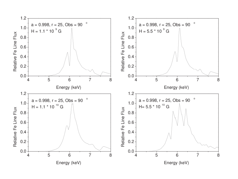
Figure 1: Spectral line shapes for $a=0.998$, $r=25$, the inclination angle of observer (Obs$=90^{\circ}$), for different magnetic fields $H=1.1\times 10^{9}$ G, $5.5\times 10^{9}$G, $1.1\times 10^{10}$ G, $5.5\times 10^{10}$G.

Fig. 1 shows a series of spectral line profiles for $a=0.998$, $r=25$ and the inclination angle of observer Obs$=90^{\circ}$ (it means that an observer is located in the equatorial plane) for magnetic fields $H=1.1\times 10^{9}$ G, $5.5\times 10^{9}$G, $1.1\times 10^{10}$ G, $5.5\times 10^{10}$G respectively. Corresponding parameter values are indicated in the left top angle of each panel. One could see from these panels that magnetic field $H=5.5\times 10^{9}$G does not distort significantly the spectral line profiles, but $1.1\times 10^{10}$G gives a significant broadening the peaks of the profile and as a result the shortest red peak may be not distinguishable from observational point of view. The spectral line profile for $H=5.5\times 10^{10}$G demonstrates a significant difference from the spectral line profile with respectively ”low” magnetic field like in first panel $H=1.1\times 10^{9}$ G, because there is an evident three peaked structure of the spectral line profile for $H=5.5\times 10^{10}$G.

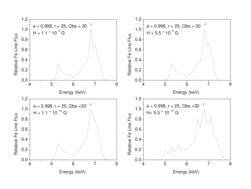
Figure 2: Spectral line shapes for $a=0.998$, $r=40$, Obs$=50^{\circ}$, for different magnetic fields $H=1.1\times 10^{9}$G, $5.5\times 10^{9}$G, $1.1\times 10^{10}$G, $5.5\times 10^{10}$G.

Fig. 2 shows a series of spectral line profiles for $a=0.998$, $r=40$ and Obs$=50^{\circ}$ and for magnetic fields $H=1.1\times 10^{9}$ G, $5.5\times 10^{9}$G, $1.1\times 10^{10}$ G, $5.5\times 10^{10}$G, respectively. In this case the magnetic field $H=5.5\times 10^{9}$G also does not distort significantly the spectral line profiles, but $H=1.1\times 10^{10}$G gives a significant broadening the profile and as a result the shortest extra blue peak is disappeared and the initial structure of the the spectral line profile with high and low blue peaks and a red peak is changed to a two-peaked structure with a red peak and a blue peak. As in Fig. 1, the spectral line profile for $5.5\times 10^{10}$G demonstrates a significant difference from the spectral line profile with respectively ”low” magnetic field like in the first panel $H=1.1\times 10^{9}$ G. This result is general for our calculations and applicable for all cases considered below.

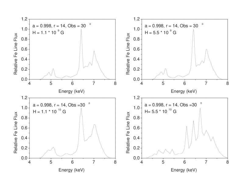
Figure 3: Spectral line shapes for $a=0.998$, $r=14$, Obs$=30^{\circ}$, for different magnetic fields $H=1.1\times 10^{9}$ G, $5.5\times 10^{9}$G, $1.1\times 10^{10}$ G, $5.5\times 10^{10}$G.

Fig. 3 shows a series of spectral line profiles for $a=0.998$, $r=14$ and Obs$=30^{\circ}$ for magnetic fields $H=1.1\times 10^{9}$ G, $5.5\times 10^{9}$G, $1.1\times 10^{10}$ G, $5.5\times 10^{10}$G, respectively. In this case the blue peak is higher than the red one (such types of peaks were calculated also by Čadež et al. (2003) for the warped disks). As for previous case (Fig. 1) magnetic field $H=5.5\times 10^{9}$G does not distort significantly the spectral line profiles, but $H=1.1\times 10^{10}$G gives a significant broadening the peaks of the profile and as a result sub-peaked structure between blue and red peaks is disappeared.

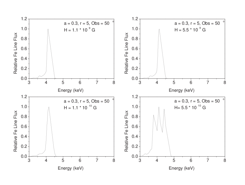
Figure 4: Spectral line shapes for $a=0.3$, $r=5$, Obs$=50^{\circ}$, for different magnetic fields $H=1.1\times 10^{9}$ G, $5.5\times 10^{9}$G, $1.1\times 10^{10}$ G, $5.5\times 10^{10}$G.

The Zeeman split of one peaked spectral line profiles is presented in Fig. 4-6. Similar spectral line profiles (without Zeeman splitting) were calculated in the framework of a warped disk model by Čadež et al. (2003) and for a cloud model by Karas et al. (2001a). Fig. 4 shows that for $a=0.3$, $r=5$ and Obs$=50^{\circ}$, there is only one single peak, but there is no bump around this peak for low magnetic fields. Fig. 5 shows that for $a=0.998$, $r=5$ and Obs$=30^{\circ}$, there is also only one single peak, but there is a broad bump around this peak for low magnetic fields (evidences for such a kind of bump was found by Wilms et al. (2001) using data of XMM-EPIC observations of MCG-6-30-15). Fig. 6 shows that for $a=0.75$, $r=5$ and Obs$=50^{\circ}$, there is also only one single peak and there is a bump around this peak for low magnetic fields. Figs. 5,6 demonstrate two cases where Zeeman splitting gives significant changes of spectral line profiles, in which evident single peak structure for low magnetic fields is changed into a three-peaked structure for high magnetic fields $H\sim 5.5\times 10^{10}$G.

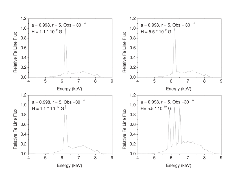
Figure 5: Spectral line shapes for $a=0.998$, $r=5$, Obs$=30^{\circ}$ for different magnetic fields $H=1.1\times 10^{9}$ G, $5.5\times 10^{9}$G, $1.1\times 10^{10}$ G, $5.5\times 10^{10}$G.

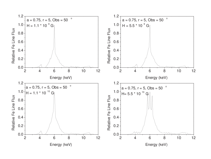
Figure 6: Spectral line shapes for $a=0.75$, $r=5$, Obs$=50^{\circ}$, for different magnetic fields $H=1.1\times 10^{9}$ G, $5.5\times 10^{9}$G, $1.1\times 10^{10}$ G, $5.5\times 10^{10}$G.

Summarizing these results of calculations for considered examples, we note that magnetic fields $H\sim 5\times 10^{10}$G produce significant changes of spectral line profiles, but $H\sim 10^{10}$ G could be responsible for essential broadening the profile peaks. Therefore, in principle there is a possibility to measure magnetic fields about $5\times 10^{10}$G that could be generated near Galactic Black Hole Candidates and probably near black hole horizons in some AGNs.

6 Summary and discussions

It is known that Fe $K_{\alpha}$ lines are found not only in AGNs and microquasars but also in X-ray afterglows of gamma-ray bursts (GRBs) (Lazzati et al., 2001). A theoretical model for GRBs was suggested recently by van Putten (2001); van Putten & Levinson (2003). In the framework of this model a magnetized torus (shell) around rapidly rotating black hole could be formed after black hole-neutron star coalescence. In this case magnetic fields could be even much higher than $10^{11}$ G. Therefore, an influence of magnetic fields on spectral line profiles can be very significant and we must take into account Zeeman splitting.

Results of 3D magnetohydrodynamical (MHD) simulations demontrated that there are non-equatorial and non-axisymmetric density patterns and some configurations like tori or shells could be formed (Mineshige et al., 2002). Moreover, an analysis of instabilities of accretion flows showed that warps, tilts and caustic surfaces could arise not only in the equatorial plane (Illarionov & Beloborodov, 2001). Observations also gave some indirect evidences for more complicated accretion flows (than the standard thin accretion flow) because there are some signatures for a precession and a nutation (for example, there is a significant precession of the accretion disk for the SS433 binary system (Cherepashchuk, 2002)).

It is evident that duplication (triplication) of a blue peak could be caused not only by the influence of a magnetic field (the Zeeman effect), but by a number of other factors. For example, the line profile can have multiple peaks when the emitting region represents multiple shells with different radial coordinates (it is easy to conclude that two emitting rings with finite widths separated by a gap, would yield a similar effect). Actually, such an explanation was proposed by Turner et al. (2002) to fit the Fe $K\alpha$ shape in NGC 3516. Despite of the fact that a multiple blue peak can be generated by many causes (including the Zeeman effect as one of possible explanation), the absence of the multiple peak can lead to a estimation of an upper limit of the magnetic field.

It is known that neutron stars (pulsars) could have huge magnetic fields. So, it means that the effect discussed above could appear in binary neutron star systems and in single neutron stars as well (Loeb, 2003). The quantitative description of such systems, however, needs more detailed computations.

Similar to considerations presented in paper by Zakharov et al. (2003), analyzing Fe $K\alpha$ shapes for MCG-6-30-15 galaxy and using ASCA data (Tanaka et al., 1995) one could evaluate a magnetic field for this case; namely a magnetic field should be less than $5\times 10^{10}$ G and the estimate is independent on a character of accretion flow. So, we could use the estimate for non-flat accretion flows for MCG-6-30-15 Seyfert galaxy and generalize conclusions by Zakharov et al. (2003) for more general cases of accretion flows.

As an extended work of the first paper by Zakharov et al. (2003), the estimates of magnetic field may seem not very precise. But one could mention that the rough estimates are caused by a noisy observational data since as a matter of fact, present spaceborne instrumentations vary greatly in their sensitivities and resolutions and precisions of measurements are not very high to have good estimates. Moreover, it would be difficult to reveal a compromisable list quantitatively of possible limiting effects restricted by different detections. However, Zakharov & Ma (2004) are trying to focus on specific ASCA observations of PKS 0637-752 in the range 1.3-24.8 keV (Yaqoob et al., 1998) and provide an estimation of the minimum magnetic field detectable with the satellite taking into account a new X-ray emission hypothesis (Varshni, 1999), other than a fluorescent assumption. The analysis is based on the laboratory measurements and identification of iron line experiments in Lawrence Livermore National Laboratory (Brown et al., 2002).

With further increase of observational facilities it may become possible to improve the above estimation. The Constellation-X launch suggested in the coming decade seems to increase the precision of X-ray spectroscopy as many as approximately 100 times with respect to the present day measurements (Weaver, 2001). Therefore, there is a possibility in principle that the upper limit of the magnetic field can also greatly improved in the case when the emission of the X-ray line arises in a sufficiently narrow region.

7 Acknowledgements

Authors are grateful to J.-X. Wang for fruitful discussions. Authors thank an anonymous referee for very useful remarks.

This work was supported by the National Natural Science Foundation of China, No.:10233050.

References

- Agol & Krolik (2000) Agol, E., & Krolik, J.H. 2000, ApJ, 528, 161.
- Ames & Thorne (1968) Ames, W. L., & Thorne K. S. 1968, ApJ, 151, 659
- Asseo & Sol (1987) Asseo, E., & Sol, H. 1987, Phys. Rep., 148, 307.
- Ballantyne & Fabian (2001) Ballantyne, D.R. & Fabian, A.C. 2001, MNRAS, 328, L11.
- Ballantyne et al. (2002) Ballantyne, D.R., Fabian, A.C., & Ross R.R. 2002, MNRAS, 329, L67.
- Balucinska-Church & Church (2000) Balucinska-Church, M., & Church, M.J. 2000, MNRAS, 312, L55.
- Berestetskii et al. (1982) Berestetskii, V.B., Lifshits, E.M., & Pitaevskii, L.P. 1982, Quantum electrodynamics, (Pergamon Press, Oxford).
- Bianchi & Matt (2002) Bianchi, S., & Matt, G. 2002, A&A, 387, 76.
- Bisnovatyi-Kogan, Lovelace & Belinski (2002) Bisnovatyi-Kogan, G.S., Lovelace, R.V.E., & Belinski, V.A. 2002, ApJ, 580, 380.
- Bisnovatyi-Kogan & Ruzmaikin (1974) Bisnovatyi-Kogan, G.S., & Ruzmaikin, A.A. 1974, A&SS, 28, 45.
- Bisnovatyi-Kogan & Ruzmaikin (1976) Bisnovatyi-Kogan, G.S., & Ruzmaikin, A.A. 1976, A&SS, 42, 401.
- Blackman & Hartnoll (2002) Blackman, E.G., & Hartnoll, S.A. 2002, in Active Galactic Nuclei: from Central Engine to Host Galaxy, ASP Conference Series, ed. S. Collin, F.Combes and I.Shlosman, 290, 79.
- Blokhintsev (1964) Blokhintsev, D.I. 1964, Quantum mechanics, (D. Reidel Publ. Co. Dordrecht, Holland).
- Boller et al. (2002) Boller, Th., Fabian, A.C., Sunyaev, R., et al. 2002, MNRAS, 329, L1.
- Bromley et al. (1997) Bromley, B.C., Chen, K., & Miller W.A. 1997, ApJ, 475, 57.
- Bromley et al. (1998) Bromley, B.C., Miller, W.A., & Pariev, V.I. 1998, Nature, 391, 54.
- Brown et al. (2002) Brown, G. V., Beiersdorfer, P, Liedahl, D. A. et al. 2002, ApJS 140, 589.
- Čadež et al. (2003) Čadež, A., Brajnik, M., Gomboc, A., Calvani M., & Fanton, C. 2003, A & A, 403, 29.
- Celotti, Fabian & Rees (1992) Celotti, A., Fabian, A.C., & Rees M.J. 1992, MNRAS, 255, 419
- Chen & Halpern (1989) Chen, K., & Halpern, J.P. 1989, ApJ, 344, 115
- Cherepashchuk (2002) Cherepashchuk, A.M. 2002, Space Sci. Rev., 102, 23
- Cherepashchuk (2003) Cherepashchuk, A.M. 2003, Physics – Uspekhi, 46, 335.
- Collin-Souffrin et al. (1996) Collin-Souffrin, S., Czerny, B., Dumont, A.-M., & Zycky, P.T. 1996, A & A, 314, 393
- Collin et al. (2003) Collin, S., Coupe, S., Dumont, A.-M., Petrucci, P.-O., & Rozanska, A. 2003, A & A, 400, 437
- Costa et al. (2001) Costa, E., Soffitta, P., Belazzini, R., et al. 2001, Nature, 411, 662
- Cui et al. (1998) Cui, W., Zhang, S.N., & Chen, W. 1998, ApJ, 257, 63
- Cunningham (1975) Cunningham, C. T. 1975, ApJ, 202, 788
- Dabrowski et al. (1997) Dabrowski, Y., Fabian, A. C., Iwasawa, K., et al. 1997, MNRAS, 288, L11
- Dirac (1958) Dirac, P.A.M. 1958, The principles of quantum mechanics, 4-th Edition, (Oxford University Press).
- Fabian et al. (1989) Fabian, A.C. Rees, M.J., Stella, L., & White, N.E. 1989, MNRAS, 238, 729
- Fabian et al. (1995) Fabian, A.C., Nandra, K., Reynolds, C.S., et al. 1995, MNRAS, 277, L11
- Fabian (1999) Fabian, A.C. 1999, MNRAS, 308, L39
- Fabian et al. (2001) Fabian, A.C. 2001, in Relativistic Astropysics, Texas Symposium, American Institute of Physics, AIP Conference Proceedings, 586, 643
- Fabian et al. (2002) Fabian, A.C., Vaughan, S., Nandra, K., et al. 2002, MNRAS, 335, L1
- Fock (1978) Fock, V.A. 1978, Fundamentals of quantum mechanics, (Mir, Moscow)
- George & Fabian (1991) George, I. M., & Fabian, A.C., 1991, MNRAS, 249, 352
- Gerlach (1971) Gerlach, U. H. 1971, ApJ, 168, 481
- Giovannini (2001) Giovannini, M., hep-ph/0111220
- Greiner (2000) Greiner, J. 2000, in ”Cosmic Explosions”, Proceedings of 10th Annual Astrophysical Conference in Maryland, eds. S.Holt & W.W.Zang, AIP Conference proceedings, 522, 307
- Hartnoll & Blackman (2000) Hartnoll, S.A., & Blackman, E.G. 2000, MNRAS, 317, 880
- Hartnoll & Blackman (2001) Hartnoll, S.A., & Blackman, E.G. 2001, MNRAS, 324, 257
- Hartnoll & Blackman (2002) Hartnoll, S.A., & Blackman E.G. 2002, MNRAS, 332, L1
- Illarionov & Beloborodov (2001) Illarionov, A.F., & Beloborodov, A.M. 2001, MNRAS, 323, 159
- Iwasawa et al. (1996) Iwasawa, K., Fabian, A. C., Reynolds, C. S., et al. 1996, MNRAS, 282, 1038
- Iwasawa et al. (1999) Iwasawa, K., Fabian, A.C., Young, A.J., et al. 1999, MNRAS, 306, L19
- Jenkins & Segre (1939) Jenkins, F.A, & Segre, E. 1939, Phys. Rev., 55, 52
- Karas et al. (2001a) Karas, V., Czerny, B., Abrassart, A., & Abramowicz, M.A. 2001a, A & A, 318, 547
- Karas et al. (2001b) Karas, V., Martocchia, A., & Subr L., 2001b, PASJ, 53, 189
- Karas et al. (1992) Karas, V., Vokrouhlicky, D., & Polnarev, A. G. 1992, MNRAS, 259, 569
- Kardashev (1995) Kardashev, N.S. 1995, MNRAS, 276, 515
- Kardashev (2001a) Kardashev, N.S. 2001a, in Quasars, AGNs and Related Research Across 2000, ed. G. Setti & J.-P. Swings, (Springer -Berlin), 66
- Kardashev (2001b) Kardashev N.S. 2001b, in Astrophysics on the edge of centuries. Proceedings of Russian astronomical conference, Pushchino, ed. N.S.Kardashev, R.D. Dagkesamanskij & Yu.A. Kovalev, (Yanus-K, Moscow) 383.
- Kardashev (2001c) Kardashev, N.S. 2001c, MNRAS, 326, 1122
- Koide et al. (2002) Koide, S., Shibata, K., Kudoh, T., et al. 2002, Science, 295, 1688
- Krolik (1999) Krolik, J.H. 1999, ApJ, 515, L73
- Krolik (2001) Krolik, J.H. 2001, in Relativistic Astropysics, Texas Symposium, American Institute of Physics, AIP Conference Proceedings, 586, 674
- Laor (1991) Laor, A. 1991, ApJ, 376, 90
- Lazzati et al. (2001) Lazzati, D., Ghisellini, G., Vietri, M., et al. 2001, in Proc. of the International workshop held in Rome, CNR headquaters, ed. E.Costa, F. Frontera & J. Hjorth (Springer, Berlin–Heidelberg) 236.
- Lee et al. (2000) Lee, J.C., Fabian, A.C., Reynolds, C.S., et al. 2000, MNRAS, 318, 857
- Lee et al. (2002) Lee, J.C., Iwasawa, K., Houck, J.C., et al. 2002, ApJ, 570, L47
- Levenson et al. (2002) Levenson N.A., Krolik J.H., Zycki P.T., et al. 2002, ApJ, 573, L81.
- Li (2002a) Li, L.-X. 2002a, A & A, 392, 469
- Li (2002b) Li, L.-X. 2002b, ApJ, 567, 463
- Liang (1998) Liang, E.P. 1998, Phys. Rep., 302, 69
- Loeb (2003) Loeb, A. 2003, PRL, 91, 071103.
- Lovelace et al. (1997) Lovelace, R.V.E., Newman, W.I., & Romanova, M.M. 1997, ApJ, 484, 628
- Lovelace et al. (1999) Lovelace, R.V.E., Li, H., Colgate, S.A., et al. 1999, ApJ, 513, 805
- Ma (2000) Ma, Z. 2000, Chinese A&A, 24, 135
- Ma (2003) Ma Z. 2003, in Proc. of the 214th Symposium on ”High Energy Processes and Phenomena in Astrophysics”, ed. X.D.Li, V. Trimble, Z.R. Wang, Astronomical Society of the Pacific, 275.
- Ma (2002b) Ma Z., 2002b, Chinese Physics Letters, 19, 1537
- Malizia et al. (1997) Malizia, A., Bassani, L., Stephen, J.B. et al. 1997, ApJS, 113, 311
- Malzac (2001) Malzac, J., 2001, MNRAS, 325, 1625
- Martocchia et al. (2002b) Martocchia, A., Matt, G., & Karas, V., 2002a, A&A, 383, L23
- Martocchia et al. (2002a) Martocchia, A., Matt, G., Karas, V. et al. 2002b, A&A, 387, 215
- Matt et al. (1992a) Matt, G., Perola, G.C., Piro, L., & Stella, L. 1992a, A&A, 257, 63
- Matt et al. (1992b) Matt, G., Perola, G.C., Piro, L., & Stella, L. 1992b, A&A, 263, 453
- Matt (2002) Matt, G. 2002, MNRAS, 337, 147
- Meier, Koide & Uchida (2001) Meier, D.L., Koide, S., & Uchida, Y. 2001, Science, 291, 84
- Merloni & Fabian (2001) Merloni, A., & Fabian, A.C. 2001, MNRAS, 321, 549
- Messia (1999) Messia, A. 1999, Quantum mechanics, (Dover, New York)
- Miller et al. (2002) Miller, J.M., Fabian, A.C., Wijnands, R., et al. 2002, ApJ, 570, L73
- Mineshige et al. (2002) Mineshige, S., Hosokawa, T., Machida, M. & Matsumoto, R. 2002, PASJ, 54, 655
- Mirabel (2001) Mirabel, I.F. 2001, Ap & SS, 276, 319
- Mirabel & Rodriguez (2002) Mirabel, I.F, & Rodriguez, L.F. 2002, Sky & Telescope, May, 33
- Morales & Fabian (2002) Morales, R., & Fabian, A.C. 2002, MNRAS, 329, 209
- Nandra et al. (1997a) Nandra, K., George, I.M., Mushotzky, R.F., et al. 1997a, ApJ, 476, 70
- Nandra et al. (1997b) Nandra, K., George, I.M., Mushotzky, R.F., et al., 1997b, ApJ, 477, 602
- Nayakshin & Kazanas (2001a) Nayakshin, S., & Kazanas, D. 2001a, ApJ, 553, L141
- Nayakshin & Kazanas (2001b) Nayakshin, S. & Kazanas, D. 2001b, ApJ, 567, 85
- Novikov & Frolov (2001) Novikov, I.D., & Frolov, V.P., 2001, Physics – Uspekhi, 44, 291
- Ogle et al. (2000) Ogle, P.M., Marshall, H.L., Lee J.C., et al., 2000, ApJ, 545, L81.
- Pariev & Bromley (1997) Pariev, V.I, & Bromley, B.C. 1997, in Proc. of the 8-th Annual October Astrophysics Conference in Maryland, Accretion Processes in Astrophysical Systems: Some Like It Hot!, ed. S.S.Holt & T. Kallmann, 273
- Pariev & Bromley (1998) Pariev, V.I., & Bromley, B.C. 1998, ApJ, 508, 590
- Pariev et al. (2001) Pariev, V.I., Bromley, B.C., & Miller W.A. 2001, ApJ, 547, 649
- Paul et al. (1998) Paul, B., Agrawal, P.C., Rao, A.R. et al., 1998, ApJ, 492, 15
- Preston (1970) Preston, G.W., 1970, ApJ, 160, L143
- Popović et al. (2001) Popović, L.C., Mediavilla, E.G., & Munoz J.A. 2001, A&A, 378, 295
- Popovic et al. (2003) Popović, L.C., Mediavilla, E.G., Jovanović, P. & Muñoz, J. 2003, A&A, 398, 975
- Reynolds & Nowak (2003) Reynolds, C.S. & Nowak, M.A. 2003, Phys. Rep., 377, 389
- Romanova et al. (1998) Romanova, M.M., Ustyugova, G.V., Koldoba, A.V., et al. 1998, ApJ, 500, 703
- Sambruna et al. (1998) Sambruna, R.M., George, I.M., Mushotsky, R.F., et al. 1998, ApJ, 495, 749
- Sazonov et al. (2002) Sazonov, S.Yu., Churazov, E.M., & Sunyaev, R.A. 2002, MNRAS, 330, 817
- Schiff & Snyder (1939) Schiff, L.I., & Snyder, H., 1939, Phys. Rev., 55, 59
- Shakura (1972) Shakura, N.I. 1972, AZh, 49, 921
- Shih et al. (2002) Shih, D.C., Iwasawa, K., & Fabian A.C. 2002, MNRAS, 2002, 333, 687
- Sulentic et al. (1998a) Sulentic, J.W., Marziani, P., Calvani, M. 1998a, ApJ, 497, L65
- Sulentic et al. (1998b) Sulentic, J.W., Marziani, P., Zwitter, T., et al. 1998b, ApJ, 501, 54
- Tanaka et al. (1995) Tanaka, Y., Nandra, K., Fabian, A.C., et al. 1995, Nature, 375, 659
- Thorne (1967) Thorne, K. S. 1967, in High Energy Astrophysics, ed. C. De Witt, E. Schatzman & P. Veron, (Science Publishers, New York) 3
- Thorne (1974) Thorne, K. S. 1974, ApJ, 191, 507
- Turner et al. (2002) Turner, T. J., Mushotzky, R.F., Yagoob, T., et al. 2002, ApJ, 574, L127
- van Putten (2001) van Putten, M.H.P.M. 2001, Phys. Rep., 345, 1
- van Putten & Levinson (2003) van Putten, M.H.P.M, & Levinson, A. 2003, ApJ, 584, 937
- Varshni (1999) Varshni, Y.P. 1999, Bull. Amer. Phys. Soc., 44, 1635.
- Vietri & Stella (1998) Vietri M., & Stella L. 1998, ApJ, 503, 350
- Wanders et al. (1997) Wanders, I., Peterson, B. M., Alloin, D., et al. 1997, ApJS, 113, 69
- Wang et al. (2003) Wang, D.-X., Lei, W.-H., Ma, R.-Y. 2003, MNRAS, 342, 851.
- Weaver et al. (1998) Weaver, K.A., Krolik, J.H., & Pier, E.A. 1998, ApJ, 498, 213.
- Weaver (2001) Weaver, K.A. 2001, in Relativistic Astrophysics, Texas Symposium, American Institute of Physics, AIP Conference Proceedings, 586, 702
- Wilkins (1972) Wilkins, D.C. 1972, Phys. Rev. D, 5, 814
- Wilms et al. (2001) Wilms, J., Reynolds, C.S., Begelman, M.C., et al. 2001, MNRAS, 328, L27
- Yaqoob et al. (1996) Yaqoob, T., Serlemitsos, P.J., Turner, T.J., et al., 1996, ApJ, 470, L27
- Yaqoob et al. (1997) Yaqoob, T., McKernan, B., Ptak, A., et al. 1997, ApJ, 490, L25
- Yaqoob et al. (1998) Yaqoob, T., George, I. M.; Turner, T. J et al.. 1998, ApJL, 505, L87.
- Yaqoob et al. (2001) Yaqoob, T., George, I.M., Nandra, K., et al. 2001, ApJ, 546, 759
- Yaqoob et al. (2002a) Yaqoob, T., George, I.M., Turner T.J., 2002a, in High Energy Universe at Sharp Focus: Chandra Science, proc. of a conference held in St. Paul, MN, 16-18 July 2001, ed. E.M. Schlegel and S.D. Vrtilek, ASP Conference Proceedings, Vol. 262 (San Francisco: Astronomical Society of the Pacific, 2002, 203
- Yaqoob et al. (2002b) Yaqoob, T., Padmanabhan, U., Dotani, T., et al., 2002b, ApJ, 569, 487
- Yu & Lu (2001) Yu, Q., & Lu, Y. 2001, A&A, 377, 17
- Zakharov (1986) Zakharov, A.F. 1986, JEThP, 91, 3
- Zakharov (1989) Zakharov, A.F. 1989, JEThP, 95, 385
- Zakharov (1991) Zakharov, A.F. 1991, Soviet Astronomy, 35, 147
- Zakharov (1993) Zakharov, A.F. 1993, Preprint MPA 755
- Zakharov (1994) Zakharov, A.F. 1994, MNRAS, 269, 283
- Zakharov (1995) Zakharov, A.F. 1995, in Annals for the 17th Texas Symposium on Relativistic Astrophysics, The New York Academy of Sciences, 759, 550
- Zakharov (2000) Zakharov, A.F. 2000, in Proc. of the XXIII Workshop on High Energy Physics and Field Theory, IHEP, Protvino, 169.
- Zakharov (2003) Zakharov, A.F. 2003, Publ. Astron. Obs. Belgrade, 76, 147.
- Zakharov et al. (2003) Zakharov, A.F., Kardashev, N.S., Lukash, V.N., & Repin, S.V. 2003, MNRAS, 342, 1325
- Zakharov & Ma (2004) Zakharov, A.F. & Ma, Z. 2004, in preparation.
- Zakharov, Popovic & Jovanovic (2004) Zakharov, A.F., Popović, L.C. & Jovanović, P., 2004, A&A, 420, 881.
- Zakharov & Repin (1999) Zakharov, A.F., & Repin, S.V. 1999, Astronomy Reports, 43, 705
- Zakharov & Repin (2001) Zakharov, A.F. & Repin, S.V., 2001, in Proc. of the XXIV International Workshop on High Energy Physics and Field Theory ”Fundamental Problems of High Energy Physics and Field Theory”, ed. V.A. Petrov, State Research Center of Russia – Institute for High Energy Physics, Protvino, p. 99 (2001).
- Zakharov & Repin (2002a) Zakharov, A.F., & Repin, S.V. 2002a, Astronomy Reports, 46, 360
- Zakharov & Repin (2002b) Zakharov, A.F., & Repin S.V. 2002b, in Proc. of the Eleven Workshop on General Relativity and Gravitation in Japan, ed. J. Koga, T. Nakamura, K. Maeda, K. Tomita, Waseda University, Tokyo, 68
- Zakharov & Repin (2002c) Zakharov, A.F., & Repin, S.V. 2002c, in Proc. of the Workshop ”XEUS - studying the evolution of the hot Universe”, ed. G. Hasinger, Th. Boller, A.N. Parmar, MPE Report 281, 339
- Zakharov & Repin (2002d) Zakharov, A.F., & Repin, S.V. 2002d, in Proc. of the XXXVIIth Rencontres de Moriond ”The Gamma-ray Universe”, ed. A. Goldwurm, D.N. Neumann and J.Tran Thanh Van, The GIOI publishers, 203.
- Zakharov & Repin (2003a) Zakharov, A.F., & Repin, S.V. 2003a, in Proc. of the Tenth Lomonosov Conference on Elementary Particle Physics ”Frontiers of Particle Physics”, ed. A.I. Studenikin, World Scientific Publishing House, Singapore, 278.
- Zakharov & Repin (2003b) Zakharov, A.F., & Repin, S.V. 2003b, A & A, 406, 7
- Zakharov & Repin (2003c) Zakharov, A.F., & Repin, S.V. 2003c, Astronomy Reports, 47, 733
- Zakharov & Repin (2003d) Zakharov, A.F., & Repin, S.V. 2003d, in Proc. of the 214th Symposium on ”High Energy Processes and Phenomena in Astrophysics”, ed. X.D.Li, V. Trimble, Z.R. Wang, Astronomical Society of the Pacific, 97.
- Zakharov & Repin (2003e) Zakharov A.F. & Repin S.V., 2003e, in Proceedings of the Third International Sakharov Conference on Physics, volume I, ed. A. Semikhatov, M. Vasiliev and V.Zaikin, Scientific World, 503.
- Zakharov & Repin (2004a) Zakharov A.F., Repin S. V., 2004a, The iron -line as a tool for a rotating black hole geometry analysis, in proc. the International Conference ”I.Ya. Pomeranchuk and physics at the turn of centuries”, World Scientific Publishing House, Singapore, 159.
- Zakharov & Repin (2004b) Zakharov, A.F., & Repin, S.V. 2004b, accepted in Adv. Space Res.
- Zamanov & Marziani (2002) Zamanov, R., & Marziani, P. 2002, ApJ, 571, L77