The Number of Supernovae from Primordial Stars in the Universe

Abstract

Recent simulations of the formation of the first luminous objects in the universe predict isolated very massive stars to form in dark matter halos with virial temperatures large enough to allow significant amounts of molecular hydrogen to form. We construct a semi-analytic model based on the Press-Schechter formalism and calibrate the minimum halos mass that may form a primordial star with the results from extensive adaptive mesh refinement simulations. The model also includes star formation in objects with virial temperatures in excess of ten thousand Kelvin. The free parameters are tuned to match the optical depth measurements by the WMAP satellite. The models explicitly includes the negative feedback of the destruction of molecular hydrogen by a soft UV background which is computed self-consistently. We predict high redshift supernova rates as one of the most promising tools to test the current scenario of primordial star formation. The supernova rate from primordial stars peaks at redshifts $\sim~{}20$. Using an analytic model for the luminosities of pair-instability supernovae we predict observable magnitudes and discuss possible observational strategies. Such supernovae would release enough metals corresponding to a uniform enrichment to a few hundred thousands of solar metalicity. If some of these stars produce gamma ray bursts our rates will be directly applicable to understanding the anticipated results from the SWIFT satellite. This study highlights the great potential for the James Webb space telescope in probing cosmic structure at redshifts greater than 20.

1. Introduction

The properties of pre-reionization luminous objects are integral to our comprehension of the process of reionization and their effect on subsequent structure formation. Observations of distant ($z=6.28,6.4$) quasars depict the relics of reionization with their accompanying Gunn-Peterson troughs (Becker et al., 2002; Fan et al., 2002). Furthermore, Lyman alpha forest carbon abundances of $\sim$10^-2Z_⊙ and 10^-3.7Z_⊙ observed at redshifts 3 and 5, respectively, indicate that numerous early supernovae (SNe) enriched the intergalactic medium (IGM) (Songaila & Cowie, 1996; Songaila, 2001). These early generations of stars are at least partly responsible for ionizing the Universe. A fraction of these stars lie in protogalaxies, but the other fraction of early stars are metal-free, form through molecular hydrogen cooling and are very massive (M $\sim$ 100$M_{\odot}$) (Abel, Bryan, & Norman, 2000; Abel, Bryan, & Norman, 2002). In $\Lambda$CDM cosmologies, these stars form at 10 $\,\buildrel<\over{\sim}\,$ z $\,\buildrel<\over{\sim}\,$ 50. The Wilkinson Microwave Anisotropy Probe (WMAP) data further constrains the epoch of reionization from the measurement of the optical depth due to electron scattering, $\tau_{es}$ = 0.17 $\pm$ 0.04 (68%), which corresponds to a reionization redshift of 17 $\pm$ 5 when assuming instantaneous reionization (Kogut et al., 2003). However in this paper, we shall show that this epoch is gradual and its effect on primordial star formation.

In hierarchical models of structure formation, small objects merge to form more massive structures. Eventually, a fraction of halos are massive ($\sim 5\times 10^{5}M_{\odot}$ at $z\sim 20$) enough to host cooling gas (Couchman & Rees, 1986; Tegmark et al., 1997; Abel et al., 1998; Fuller & Couchman, 2001). These halos do not cool through atomic line cooling since $T_{vir}<10^{4}$; however, primordial gas contains a trace of H₂. Free electrons which allow molecular hydrogen to form that acts as an effective coolant at several hundred degrees through rotational and vibrational transitions. H₂ is easily photo-dissociated by photons in the Lyman-Werner (LW) band, 11.26–13.6eV (Field, Somerville, & Dressler, 1966; Stecher & Williams, 1967), thus H₂ can be destroyed by distant sources in a neutral Universe. Primordial stars produce copious amounts of UV photons in the LW band, destroying the most effective cooling process at $z\sim 20$. This negative feedback from the UV background significantly inhibits the primordial star formation rate in the early universe by requiring a larger potential well for gas to condense. Many groups have explored the effects of a UV background on cooling and collapsing gas. Firstly, Dekel & Rees (1987) discovered that H₂ can be dissociated from large distances. Then more quantatively, Haiman, Rees, & Loeb (1997) questioned how the collapse homogeneous, spherical clouds are affected by a UV background. In more detail, Haiman, Abel, & Rees (2000) determined whether a gas cloud collapsed by comparing the cooling time with the current lifetime of the cloud, which was calculated in the presence of solving the spherically symmetric radiative transfer equation along with time-dependent H₂ cooling functions. However, these studies only considered spherically symmetric cases while realistically these halos are overdensities within filaments. To combat this problem, Machacek, Bryan, & Abel (2001) employed a three-dimensional Eulerian adaptive mesh refinement (AMR) simulation to determine quantitative effects of a UV background on gas condensation.

We consider lower mass stars to form in more massive halos that may fragment via atomic line cooling as well as the metal lines from the heavy elements expelled by the earlier generation of Pop III stars. We use the prescription outlined in Haiman & Loeb (1997) (hereafter HL97) to model the abundances and luminosities of these stars.

With infrared space observatories, such as the Spitzer Space Telescope, Primordial Explorer (PRIME; Zheng et al., 2003), and James Webb Space Telescope (JWST), sufficient sensitivity is available to detect the SNe from primordial stars. Although SNe remnants are bright for short periods of time, they may be the best chance to directly observe primordial stars due to their large intrinsic luminosities. If these events are recorded, many properties, such as mass, luminosity, metallicity, and redshift, of the progenitors can be calculated using metal-free or ultra metal-poor SNe models, which can validate or falsify simulations of the first stars (Abel, Bryan, & Norman, 2002). To evolve our calculation through redshift, we need to retain information about the UV background and number densities of primordial stars, which can extend to determining such quantities as volume-averaged metallicity and ionized fraction of the Universe. Our model is constrained with (a) the WMAP optical depth measurement, (b) primordial star formation and suppression in high resolution hydrodynamical simulations, and (c) local observations of dwarf galaxies that constrain high redshift protogalaxies properties.

We organize the paper as follows. In §2, we report the semi-empirical method behind our calculations, which incorporates effects from negative feedback and an ionized fraction and is constrained from the WMAP result and local dwarf galaxy observations. In §3, we present the number density of primordial SNe in the sky and the evolution of SNe rates, metallicity, and related SNe quantities. We also explore the feasibility of observing these SNe by calculating their magnitudes and comparing them with the sensitivities of infrared space observatories. Then in §4, we suggest possible future observations and numerical simulations that could further constrain our model. Finally, §5 discusses and summarizes our results and the implications of the first observations of SNe from primordial stars.

2. The Method

We use several theories and results from simulations of structure formation and metal-free stars. We use a $\Lambda$CDM cosmology with $\Omega_{\Lambda}$ = 0.70, $\Omega_{\rm{CDM}}$ = 0.26, $\Omega_{b}$ = 0.04, h = 0.7, $\sigma_{8}$ = 0.9, and n = 1. $\Omega_{\Lambda}$, $\Omega_{\rm{CDM}}$, and $\Omega_{b}$ are the fractions of mass-energy contained in vacuum energy, cold dark matter, and baryons, respectively. $h$ is the Hubble parameter in units of 100 km s^-1 Mpc^-1. n = 1 indicates that we used a scale-free power spectrum, and $\sigma_{8}$ is the variance of random mass fluctuations in a sphere of radius 8h^-1 Mpc. We use a CDM power spectrum defined in Bardeen et al. (1986), which depends on $\sigma_{8}$ and h.

The remaining parameters are the primordial stellar mass, and the factors f_esc and f_⋆, which dictates the production and escape of ionizing photons, where f_esc is the photon escape fraction, and f_⋆ is the star formation efficiency.

To evolve the ionization and star formation behaviors of the Universe, we must determine the density of dark matter halos that host early stars. In $T_{vir}<10^{4}$ K halos (henceforth “minihalos”), H₂ cooling is the primary mechanism that provides means of condensation into cold, dense objects. However in $T_{vir}>10^{4}$ K, which corresponds to $M_{vir}>10^{8}M_{\odot}[(1+z)/10]^{-3/2}$, halos, hydrogen atomic line cooling allows the baryons to fragment and cool into stars.

2.1. Minihalo Star Formation

The first quantity we need to begin our calculation is the minimum halo mass that forms a cold, dense gas core due to H₂ cooling. Radiation in the LW band photo-dissociates H₂, which inhibits star formation in minihalos. This negative feedback from a UV background does not necessarily prohibit the formation of primordial stars in minihalos, but only increases the critical halo mass in which condensation occurs, and delays the star formation. From their simulations of pre-galactic structure formation, Machacek, Bryan, & Abel (2001) determined the minimum mass of halo that hosts a massive primordial star is

$$\frac{M_{min}}{M_{\odot}}=\exp\left(\frac{f_{cd}}{0.06}\right)\left(1.25\times 10^{5}+8.7\times 10^{5}F_{LW,-21}^{0.47}\right),$$ (1)

where $M_{min}$ is the minimum halo mass that contains a cold, dense gas core, $f_{cd}$ is the fraction of gas that is cold and dense, and $F_{LW}$ is the flux within the LW band in units of 10^-21 erg^-1 s^-1 cm^-2 Hz^-1. For our calculation, we consider $f_{cd}=0.02$, which is a conservative estimate in which we have an adequate source of star forming gas. With our chosen $f_{cd}$ and no UV background, a 1.74 $\times$ 10⁵ $M_{\odot}$ halo will form a cold, dense core, which will continue to form a primordial star. In a typical UV background of J = 10^-21 erg^-1 s^-1 cm^-2 Hz^-1 sr^-1, the minimum mass is 4.16 $\times$ 10${}^{6}M_{\odot}$. Additionally, minihalos can only form a star within neutral regions of the Universe since they are easily photoionized (Haiman, Abel, & Madau, 2001; Oh & Haiman, 2003) and H I is a necessary ingredient for producing H₂.

Numerical simulations (e.g. Abel, Bryan, & Norman, 2002; Bromm, Coppi, & Larson, 2002) illustrated that fragmentation within the inner molecular cloud does not occur and a single massive (M $\sim$ 100$M_{\odot}$) star forms in the central regions. These stars produce hard spectra and tremendous amounts of ionizing photons. For example, the ionizing photon to stellar baryon ratio n_γ $\sim$ 91300, 56700, and 5173 for H, He, He⁺ in a 200$M_{\odot}$ star (Schaerer, 2002). We calculate the ionizing photon flux by considering

$$\left(\frac{dN_{\gamma}}{dt}\right)_{mini}=\bar{Q}\>T_{life}\>\frac{d\rho_{mini}}{dz}\>\frac{dz}{dt},$$ (2)

where Q is the time-averaged photon flux, T_life is the stellar lifetime, and $\rho_{mini}$ is the comoving number density of minihalos that we determine from an elliposdial variant of Press-Schechter (PS) formalism (Press & Schechter, 1974; Sheth & Tormen, 2002).

The primordial initial mass function (IMF) is unknown, therefore, we assume a fixed primordial stellar mass for each calculation. We run the model for primordial stellar masses, M_fs, of 100, 200, and 500 $M_{\odot}$ and use the time-averaged emissivities from metal-free stellar models with no mass loss (Schaerer, 2002). In our models, the minihalo is quickly ionized and all photons escape into the IGM (Whalen, Abel, & Norman, 2004). Furthermore, we use a blackbody spectrum at 10⁵ K to approximate the spectrum of the primordial star to consider the flux in the LW band since surface temperatures are virtually independent of mass at M $\,\buildrel>\over{\sim}\,$ 80$M_{\odot}$.

2.2. Star Formation in Protogalaxies

In $T_{vir}>10^{4}$ K halos, baryons can cool efficiently through atomic line cooling, thus fragmenting and forming stars. As described in HL97, we parameterize the properties of these stars by a couple of factors.

2.2.1 Star formation efficiency

High redshift galaxies appear to have similar properties as local dwarf galaxies. We can constrain the star formation efficiency f_⋆ by letting local observations guide us. In these galaxies, f_⋆ range from 0.02 to 0.08 (Taylor et al., 1999; Walter et al., 2001). Using the orthodox Schmidt star formation law, Gnedin (2000) estimated f_⋆ to be 0.04 if it was constant over the first 3 Gyr but can also be as low as 0.022. It should be noted that f_⋆ can be higher if star formation ceased after a shorter initial burst.

Analyses of metallicities in local dwarf galaxies reveal their prior star formation. Both Type Ia and Type II SNe contribute iron to the IGM, but Type II SNe provide most of the $\alpha$-process elements (e.g. C, N, O, Mg) to the IGM. Type II SNe occur on timescales $<3\times 10^{7}$ yr while Type Ia are delayed by $3\times 10^{7}$ yr to a Hubble time (Matteucci & Recchi, 2001). Therefore, we expect an overabundance of $\alpha$-process elements with respect to iron. [$\alpha$/Fe] versus [Fe/H] plots help us inspect the evolution of the ISM/IGM metallicity. If the prior star formation is inefficient (spirals, irregulars), [$\alpha$/Fe] is only shortly overabundant, which is characterized by a short plateau versus [Fe/H]. On the other hand, if the star formation is fast and occurs early in the lifetime of the galaxy, [$\alpha$/Fe] remains in the plateau longer due to the quick production of metals within Type II SNe (see Figure 1 in Matteucci, 2002). Recently, Venn et al. (2003) discovered no apparent plateau in [$\alpha$/Fe] versus [Fe/H] in dwarf spheroidal and irregular galaxies. They conclude that star formation must have been on timescales longer than Type Ia SNe enrichment, which hints at a low and continuous star formation rates in these protogalaxies when compared to recent star formation.

These low star formation efficiencies are further supported by the galaxies contained in the Sloan Digital Sky Survey (SDSS; York et al., 2000). Star formation efficiencies within low mass galaxies (M $<$ 3 $\times$ 10${}^{10}M_{\odot}$) decline as M^2/3 (Kauffmann et al., 2003). At high redshift and before reionization, most of the protogalaxies tend to be few $\times$ 10⁷ $M_{\odot}$, which is comparable to many local dwarf galaxies (Mateo, 1998). It should also be noted that even within individual Local Group galaxies no star formation history is alike, but it is worthwhile to adopt a global star formation efficiency and observe the consequences on reionization and primordial star formation. With the stated constraints, we take f_⋆ = 0.04 in our main model in concordance with the Schmidt Law (Gnedin, 2000) and stellar abundances (Venn et al., 2003).

Table 1Ionizing photon production per stellar baryon and luminosities for metal-poor IMFs

Z	n${}_{\gamma,\>H}$	n${}_{\gamma,\>He}$	n${}_{\gamma,\>He^{+}}$	log $\cal{L}$
				[erg s-1 M${}_{\odot}^{-1}$]
10-7	20102	8504	8	36.20
10-5	15670	5768	0.2	36.16
0.0004	13369	3900	0	36.28

2.2.2 Stellar luminosities

We considered several IMFs for star formation within protogalaxies. Our main model uses a Salpeter IMF with a slope $\alpha$ = –2.35, metallicity Z = 10^-7, 10^-5, and 0.0004, and (M_low, M_up) = (1, 100)$M_{\odot}$. We take the continuous starburst spectrum evolution from this particular IMF that was calculated with Starburst99 (Schaerer, 2003; Leitherer et al., 1999). To estimate the ionizing photon per stellar baryon ratio, n_γ, and luminosities of the IMF at a particular metallicity, we interpolate in log₁₀ space between the two adjacent IMFs. When Z $<$ 10^-7, then we consider the Z = 10^-7 IMF. The properties of these IMFs are listed in Table 1. Note that more metal-rich starbursts result in a softer spectrum and less ionizing photons in which n${}_{\gamma,\>H}$ decreases almost by a factor of 2.

In the Z = 0.0004 IMF, we retain the luminosity from the Z = 10^-5 and set n${}_{\gamma,\>He^{+}}$ = 0. We choose to do so because of the theoretical uncertainty of hot Wolf-Rayet (WR) stars and their presence (for a review, see Schaerer, 2000). In Schaerer (2003), the luminosity and spectral hardness increases due to the presence of hot Wolf-Rayet (WR) stars at higher metallicities. However, Smith, Norris, & Crowther (2002) calculate hot WR spectra that are significantly softer.

2.2.3 Ionizing photon escape fraction

Radiation emitted by these stars have a probability $f_{esc}$ to escape from the protogalaxy and ionize the IGM. The protogalaxy ISM density and composition plays the biggest role in determining this factor. Heckman et al. (2001) showed that local and distant starburst galaxies, including the gravitationally lensed galaxy MS 1512-cB58 (z = 2.7), have $f_{esc}$ $\,\buildrel<\over{\sim}\,$ 0.06. This result agrees with previous analyses of the $f_{esc}$ in the Lyman continuum (Leitherer et al., 1995; Hurwitz, Jelinsky, & Dixon, 1997). However, Lyman break galaxies may have higher $f_{esc}\lower 3.00003pt\hbox{$\,\buildrel>\over{\sim}\,$}0.2$ (Steidel, Pettini, & Adelberger, 2001). In conjunction with f_⋆ = 0.04 and M_fs = [100, 200, 500]$M_{\odot}$, the choice of f_esc = [0.050, 0.033, 0.028], respectively, in our calculation results in the same optical depth from WMAP, $\tau_{es}$ = 0.17, thus we use these values in the main models. Wood & Loeb (2000) and Ricotti & Shull (2000) have argued that the escape fraction may be very small due to the much higher densities at high redshift. However, the shallow potential wells and their small size make them also susceptible to photo-evaporation and effects of radiation pressure (Haehnelt, 1995). Other uncertainities such as dust content, metallicity, and whether the ISM density scales as (1+z)³ blur our intuition about the escape of ionizing radiation. Therefore, we allow $f_{esc}$ to vary from 0.001–0.25 since it is unclear whether high-redshift, low-mass protogalaxies allow photons to escape due to self-photoevaporation or absorb the photons due to a higher proper gas density when compared to starburst galaxies.

2.2.4 Ionizing Photon Rates

These factors are multiplicative in amount of radiation that is available from protogalaxies to ionize the IGM. The rate of photons emitted that can ionize species X is

$$\left(\frac{dN_{\gamma}}{dt}\right)_{proto}=\rho_{0}(1+z)\frac{f_{esc}\>f_{\star}\>n_{\gamma,X}}{\mu\>m_{p}}\>\frac{d\psi_{proto}}{dz}\frac{dz}{dt},$$ (3)

where $\mu$ is the mean molecular weight, $\rho_{0}$ = $\Omega_{b}$(3H${}_{0}^{2}$/8$\pi$G), $m_{p}$ is the mass of a proton, and $\psi_{proto}$ is the mass fraction contained in protogalaxies that is calculated by PS formalism. We restrict the product of $f_{esc}$ and $f_{\star}$ to be in a range from 10^-4–10^-2 since the resulting reionization histories fall within the measured $\tau_{es}$. The reionization epoch greatly depends on the factors $f_{esc}$ and $f_{\star}$. In order to explore the consequences of different values of $\tau_{es}$ and their resulting SNe rates, we vary the factors f_esc and f_⋆.

Figure 1.— The dashed line is the gas clumping factor as calculated in our adiabatic hydrodynamical AMR simulation. Using equation (6), we estimate the clumping factor in the ionized region to be solid line.

Figure 2.— (Clockwise from upper right) Primordial SNe rates (yr^-1 deg^-2) per unit redshift; Cumulative primordial SNe rate (yr^-1 deg^-2); Specific intensity (erg^-1 s^-1 cm^-2 Hz^-1 sr^-1) in the LW band; Comoving density (Mpc^-3) of halos above the critical star formation mass in neutral regions; Critical halo mass ($M_{\odot}$) for primordial star formation. The solid, dotted, and dashed lines correspond to calculations run with a fixed primordial stellar mass of 100, 200, and 500 $M_{\odot}$, respectively.

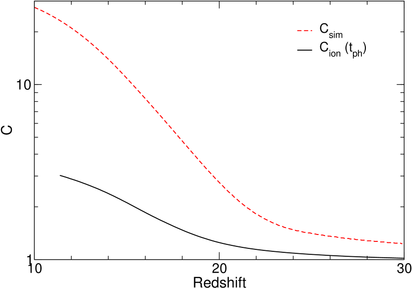
2.3. Clumping Factor

Overdense regions experience an increased recombination rate. Overdensities are characterized by the gas clumping factor C = $\langle n_{H}^{2}\rangle/\langle n_{H}\rangle^{2}$, and the recombination rate is increased by this factor. To calculate this parameter in our model, we utilize the same cosmological Eulerian AMR code enzo (Bryan & Norman, 1999) as in Machacek, Bryan, & Abel (2001) in a 256³ simulation with a comoving box side of 500kpc, eight levels of refinement, and the previously specified cosmological parameters. A total (gas) mass resolution of 1013 (135) $M_{\odot}$ results from the resolution in the top grid, which is smaller than the cosmological Jeans mass (4). Thus, we account for all collapsed halos in our clumping factor calculation. The simulation is purely adiabatic with no background radiation or atomic/molecular cooling. We show C_sim in Figure 1. Cooling only affects localized regions of star formation and does not contribute greatly in the boosting of C. However, ionizing radiation causes photoevaporation of halos, which decreases C in the process (Haiman, Abel, & Madau, 2001). We correct for photoevaporation by considering all minihalos with M_J $<$ M $<$ M_min are photoevaporated in the ionized regions of the Universe, where

$$M_{J}\approx 10^{4}\left(\frac{\Omega_{M}h^{2}}{0.15}\right)^{-1/2}\left(\frac{\Omega_{b}h^{2}}{0.02}\right)^{-3/5}\left(\frac{1+z}{11}\right)^{3/2}M_{\odot}$$ (4)

is the cosmological Jeans mass. For simplicity, we assume the IGM has a clumping factor of unity although underdense regions in the IGM correspond to C_IGM $\,\buildrel<\over{\sim}\,$ 1. We concentrate on the gas clumping factor in the ionizing regions since the goal is to calculate the increase in recombination rates. Consider an ionized region whose volume filling fraction F_H is increasing. The expansion will incorporate unaffected, clumpy material into the region. The first term in (6) accounts for this effect. Any overdensities in the ionized region will be photoevaporated in approximately a sound crossing time of the halo,

$$t_{ph}\approx\beta\frac{R_{vir}}{10{~{}{\rm km~{}s^{-1}}}},$$ (5)

where $\beta$ is a normalization factor that accounts for the differences in halo densities at various redshifts and masses and R_vir is the mean virial radius of halo with M_J $<$ M $<$ M_min (Haiman, Abel, & Madau, 2001). Since $\beta$ remains within $\sim$15% of unity for minihalos, we infer $\beta$ = 1. The photoevaporation of overdensities is the second term in the evolution of the gas clumping factor, which is

$$\dot{C}=C_{sim}\dot{F}_{H}-\frac{C-1}{t_{ph}}.$$ (6)

The effect from photoevaporation is illustrated in Figure 1. Overdensities that are engulfed by ionized regions cannot sufficiently increase the gas clumping factor to overcome the photoevaporation that occurs, and C remains within the range 1–3 for the entire calculation in our main model. This equation is weakly sensitive to t_ph since varying t_ph by a factor of 6 alters C only by a factor of 2. In a later paper, we shall computationally address the effect of radiation on the clumping factor.

2.4. The Evolution of UV Background and Halo Densities

We initialize the following method at z = 75 with no UV background, evolve the cosmological radiative transfer equation (8) at the questioned redshift, and repeat the described procedure until cosmological hydrogen reionization occurs.

Given a minimum mass of a star-forming halo, we can exploit PS formalism to calculate number densities of these halos. For minihalos, we calculate their number densities for halos with masses above M_min (1) and virial temperatures below 10⁴ K. Likewise, the protogalaxy mass fraction is calculated by considering all halos more massive than a corresponding T_vir = 10⁴ K.

We choose a variant of PS formalism, which is an ellipsoidal collapse model that is fit to numerical simulations (Sheth & Tormen, 1999; Sheth, Mo, & Tormen, 2001; Sheth & Tormen, 2002). This model is concisely summarized in Mo & White (2002). In minihalos, it is reasonable to assume one star forms per halo since E_bind $\,\buildrel<\over{\sim}\,$ E_SNe, where E_bind and E_SNe are the binding energy of the host halo and kinetic energy of the primordial SNe, respectively. The gas is totally disrupted in the halo and requires $\sim$100Myr $\ll$ t_H, where t_H is the Hubble time, to re-collapse (Abel, Bryan, & Norman 2002, unpublished). On main sequence, primordial stars evacuate large Strömgren spheres on the order of kpcs (Whalen, Abel, & Norman, 2004). Therefore,

$$\frac{d\rho_{\star}}{dz}=\frac{d\rho_{mini}}{dt}\frac{dt}{dz},$$ (7)

where $\rho_{\star}$ is the comoving density of primordial stars. With that in mind, we can calculate the volume-averaged emissivity (11) of the Universe by using metal-free stellar models (Schaerer, 2002) and the prescription outlined in §2.2 for minihalos and protogalaxies, respectively.

We evolve the spectrum from early stars to investigate how the UV background behaves, particularly in the LW band, with the cosmological radiative transfer equation,

$$\left(\frac{\partial}{\partial t}-\nu H\frac{\partial}{\partial\nu}\right)J=-3HJ-c\kappa J+\frac{c}{4\pi}\epsilon,$$ (8)

where $H=H(z)=100hE(z)$ is the Hubble parameter, and $E(z)=\sqrt{\Omega_{\Lambda}+\Omega_{m}(1+z)^{3}}$. $J=J(\nu,z)$ is specific intensity in units of erg^-1 s^-1 cm^-2 Hz^-1 sr^-1. $\kappa$ is the continuum absorption coefficient per unit length, and $\epsilon=\epsilon(\nu)$ is the proper volume-averaged emissivity (Peebles, 1993). The emissivity will be the current total luminosity per unit volume of early stars, which can be expressed as

$$\epsilon_{mini}(\nu)=\rho_{mini}\times L(\nu)\times f(\nu)\times\left(1-\frac{n_{HII}}{n_{H}}\right),$$ (9)

$$\epsilon_{proto}(\nu)=\nu^{-1}\rho_{0}\frac{d\psi_{proto}}{dt}\times L(\nu,f_{\star})\times f(\nu),$$ (10)

$$\epsilon(\nu)=(1+z)^{3}\left[\epsilon_{mini}(\nu)+\epsilon_{proto}(\nu)\right],$$ (11)

where f (13) is a factor that accounts for absorption from Lyman series transitions. L is the luminosity of the object and is defined as

$$L(\nu)=\left\{\begin{array}[]{r@{\quad}l}4\pi R^{2}B_{\nu}(T=10^{5}K)&{\rm(mini)}\\ f_{O\star}f_{\star}\mathcal{L}\frac{B_{\nu}(T=23000K)}{B_{\nu}(\nu=2.7kT/h_{p};\>T=23000K)}&{\rm(proto)}\end{array}\right.,$$

where B_ν is a blackbody spectrum, and $\cal{L}$ is listed in Table 1. R is the radius of the primordial star (Schaerer, 2002). f_O⋆ is the fraction of O stars in the starburst (Schaerer, 2003). k and h_p are Boltzmann’s constant and Planck’s constant, respectively. For the protogalaxies, T $\sim$ 23000K because the spectrum in the LW band will be dominated by OB stars, and we weight the luminosity by this blackbody spectrum. This effect and the increasing UV background effectively squelches minihalo star formation. Emissivity will be nearly zero above 13.6eV in the neutral Universe due to the hydrogen and helium absorption.

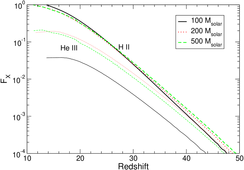
Photons from primordial stars and protogalaxies between 13.6eV and several keV ionize the surrounding neutral medium. Using the intrinsic $\geq$13.6eV ionizing photon rates from primordial stars (2) and protogalaxies (3), we calculate a volume-averaged neutral fraction. The change of ionized hydrogen comoving density due to photo-dissociation and recombination is

Figure 3.— The red dashed line is an example unprocessed spectrum of a continuous source of radiation. After being absorbed and re-emitted by Lyman-series transitions, it transforms into the “sawtooth” spectrum (black solid line). This particular spectrum is for z_on = 30 and z_obs = 20.

$$\frac{dn_{HII}}{dt}=-\frac{dN_{\gamma}}{dt}+Ck_{rec}(1+z)^{3}n_{H}^{2}\left(1-\frac{n_{HII}}{n_{H}}\right)^{2},$$ (12)

where n_HII and n_H = 0.76$\rho_{0}$/m_p are the ionized and total hydrogen comoving density, C is the clumping factor, and k${}_{rec}=$ 2.6 $\times$ 10^-13 s^-1 cm^-3 is the case B recombination rate of hydrogen at T $\approx$ 10⁴.

In the case for helium, $k_{rec}$ is approximately equal to the hydrogen case, but since the helium number density is less than hydrogen, less recombinations occur. Naïvely, this will result in a higher He⁺ fraction than H⁺ due to the hardness of the primordial radiation. Realisticly when the ionizing photons reach the ionization front, they will ionize either helium or hydrogen since hydrogen still has a finite photo-ionization cross-section above 23.6eV. We consider the He⁺ regions to be equal to the H⁺ regions. Then we add N${}_{\gamma,\>He}$ to N${}_{\gamma,\>H}$ to compensate for this effect. We perform a similar analysis on the double ionization of helium in which k${}_{rec,\>He^{+}}$ = 1.5 $\times$ 10^-12 s^-1 cm^-3 but we evaluate equation (12) directly with N${}_{\gamma,\>He^{+}}$.

Figure 4.— (Top graph) The thick solid line is the volume-averaged metallicity from protogalaxies and primordial stars in the 200$M_{\odot}$ model. The thin dotted, solid, and dashed lines are volume-averaged metallicities from 175, 200, 250 $M_{\odot}$ primordial stars only. (Bottom graph) Iron abundance relative to solar. Legend is the same as the top graph. The large spread in iron from primordial stars arises from the steep dependence of iron ejecta versus mass in pair instability SNe.

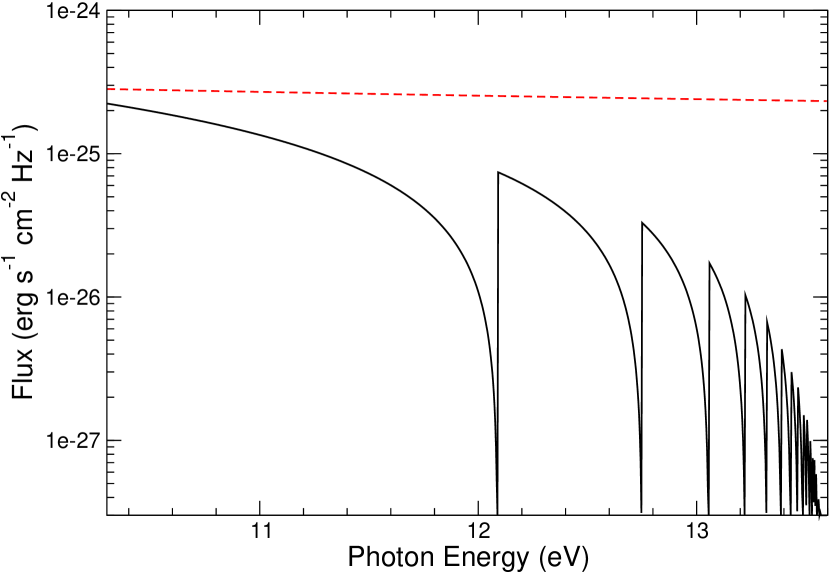
The absorption coefficient in Equation (8) is ignored since we take into account the Lyman series line absorption by the following procedure. Photons with 11.26eV $<$ E $<$ 13.6eV escape into the IGM, which will photo-dissociate H₂. To calculate the flux within the LW band, we must consider the processing of photons by the Lyman series transitions (Haiman, Rees, & Loeb, 1997). Before reionization, these transitions absorb all photons at their respective energies. These absorbers can be visualized as optically thick “screens” in redshift space, for which the photon must have been emitted after the farther wall in redshift. This process creates a sawtooth spectrum with minimums at redshift screens, which is illustrated in Figure 3. For instance, an observer at $z=20$ observes photons at 12.5eV; it must have been emitted by the Ly$\gamma$ line at 12.75eV at $z=20.4$. The fraction of photons that escape from these walls during an integration step is

$$f=\frac{1-[(1+z)/(1+z_{screen})]^{1.5+\alpha}}{1-[(1+z)/(1+z+\Delta z)]^{1.5+\alpha}},$$ (13)

where $\alpha$ = –1.8 is the slope of a power-law spectrum ($F_{\nu}\propto\nu^{-\alpha}$) and

$$z_{screen}=\frac{\nu}{\nu_{Lyi}}(1+z_{obs})-1.$$ (14)

$\nu_{Lyi}$ is the nearest, blueward Lyman transition to $\nu$. Inherently, $z_{screen}$ must be between $z$ and $z+\Delta z$.

3. Results

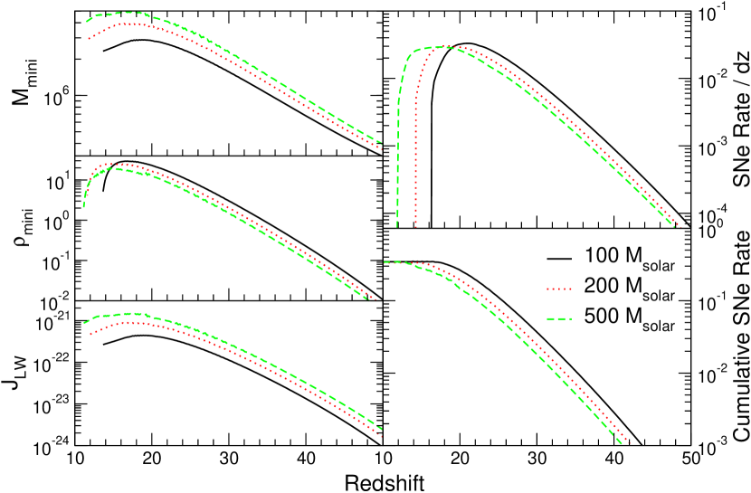
In this Section, we present the results of our calculation of the evolution of SNe rates, volume-averaged metallicity, and UV background. We also present the variance of optical depth to electron scattering and SNe rates with different protogalaxy star formation scenarios. In Figure 2, we plot minimum halo mass, density of those halos, metallicity, SNe rate, and UV background in the LW band for the main models.

Figure 5.— Evolution of filling factors of ionized hydrogen (top) and doubly ionized helium (bottom). The legend is the same as Figure 2.

3.1. Metallicity

Metal-free stars with masses between $\sim$140–260$M_{\odot}$ result in a SNe that is visible and eject heavy elements into the IGM. When a star is within this range, the stellar core has sufficient entropy after helium burning to create positron/electron pairs. These pairs convert the gas energy into mass while not greatly contributing to pressure. This creates a major instability, where the star contracts rapidly until oxygen and silicon implosive burning occurs. Then the star totally disrupts itself by these nuclear explosions (Barkat, Rakavy, & Sack, 1967; Bond, Arnett, & Carr, 1984). Stars between $\sim$100–140$M_{\odot}$ experience this instability. It is not violent enough to disrupt the star, but pulsations and mass loss occur until equilibrium is reached and the hydrogren envelope is ejected (Bond, Arnett, & Carr, 1984; Heger & Woosley, 2002). Then since it creates a large iron core, it probably forms a black hole, preventing any further ejecta. Additionally, metal-free stars above M $\,\buildrel>\over{\sim}\,$ 260$M_{\odot}$ may result in direct black hole formation, which prohibits any significant heavy element ejecta and afterglow (Fryer, Woosley, & Heger, 2001).

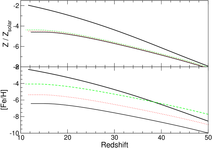
For primordial stars in the pair-instability SNe mass range, we determine a metallicity using our SNe densities and the metal production of these SNe (Heger & Woosley, 2002). Except for iron, significant spread in metallicity is not apparent for different choices of primordial stellar mass. Iron ejecta in pair instability SNe range from 0.003–57$M_{\odot}$, so naturally we expect a large spread. For star formation in protogalaxies, we use carbon and metal production values from Renzini & Voli (1981) for 1–8 $M_{\odot}$ and Maeder (1992) for 9–120 $M_{\odot}$. Additionally for 15–25$M_{\odot}$, we use the iron nucleosynthesis yields from Rauscher et al. (2002). At low metallicities and above $\sim$40$M_{\odot}$, direct black hole formation occurs after stellar collapse, which inhibits any ejecta from escaping the remnant. Furthermore above $\sim$25$M_{\odot}$, a black hole forms through “fallback” of ejecta onto the neutron star remnant (Fryer, 1999). Thus we set an upper mass cutoff of 25$M_{\odot}$ for metal enrichment from protogalaxies. With the chosen Salpeter IMF, 2.9 $\times$ 10^-3, 0.023 and 0.071 $M_{\odot}$ of iron, carbon, and metals, respectively, are produced for every $M_{\odot}$ of stellar material. It should be noted that most of the carbon is produced by intermediate mass stars, and its injection is delayed by a few hundred million years, which corresponds to the first metal enriched, intermediate mass stars exploding at z $\sim$ 12. Furthermore, we ignore the delay time of any stellar lifetimes in Figure 4 to give a rough estimate of the volume-averaged metallicity evolution.

With the evolution of metallicity, we can estimate the period of metal-poor (–5 $\,\buildrel<\over{\sim}\,$ [Fe/H] $\,\buildrel<\over{\sim}\,$ –1) star formation. For the most metal deficient stars, their metallicities of [Fe/H] = (–4.0, –5.3) correspond to a formation epoch of z $\sim$ (28, 36) (Norris, Ryan, & Beers, 2001; Christlieb et al., 2002). Additionally, primordial stars in the 200$M_{\odot}$ model account for [Fe/H] $\sim$ –5.4 of the total iron ejecta. If we set the primordial stellar mass to be 250$M_{\odot}$, these stars eject tremendous amounts of iron into the IGM and possibly enhance [Fe/H] to –4.1. Conversely, primordial stars at the lower mass range of pair-instability SNe produce insignificant amounts of iron and will not pollute the IGM. The IGM iron contribution from primordial stars is likely lower than these quoted values since in a proper IMF not all stars will result in a pair instability SNe.

Possibly these metallicities correspond to the VMS (Very Massive Star) component of metallicity of metal-poor (–4 $<$ Z/Z_⊙ $<$ –1) stars (Qian & Wasserburg, 2002). They assume that a VMS contributes 10^-4Z_⊙ to the IGM. By inspection of the evolution of metal yields from protogalaxies and primordial stars, the VMS component may contain contributions from protogalaxies since primordial stars are suppressed by the UV background before producing a universal metallicity of 10^-4Z_⊙. Lastly, metallicities found in z $\sim$ 5 Lyman alpha clouds are [C/H] $\sim$ –3.7 and much less than our calculated values (Songaila, 2001). The bulk of the metals might not migrate to the void in which Ly$\alpha$ clouds exist, and the host galaxies would retain the majority of the metals. This behavior may explain the lack of metals observed in Ly$\alpha$ clouds and the higher than expected metallicity in the VMS component. However, the clustering of the first objects, primordial IMF, and the mixing of metals in the IGM will have to be taken into account before we can predict metallicities of the Lyman alpha forest and metal deficient stars with high confidence.

Figure 6.— Using the decay of ⁵⁶Ni and Equation (20), we calculate the luminosity of primordial SNe and its effective temperature. Heavy (top) lines with circles are luminosities and light (bottom) lines are temperature. The blue dashed line with filled squares is a Type Ia luminosity evolution for comparison (Woosley & Weaver, 1986). The lines from top to bottom (dotted, solid, dashed) are for stellar masses 175, 200, and 250 $M_{\odot}$.

3.2. Optical Depth to Electron Scattering

Optical depth due to electron scattering (15) is a good observational test to determine the neutral fraction of the Universe before reionization. The WMAP satellite measured $\tau_{es}$(z) = 0.17 $\pm$ 0.04 at 68% confidence.

$$\tau_{es}(z)=\int^{z}_{0}\bar{n}_{e}\sigma_{TH}c\left(\frac{dt}{dz}\right)dz,$$ (15)

where $n_{e}$ is the proper electron density and $\sigma_{TH}$ is the Thomson cross-section. To accurately calculate $n_{e}$, we must consider all ionizations of primordial gas, which includes H⁺, He⁺, and He⁺⁺. Therefore, the proper electron density is

$$n_{e}=(1+z)^{3}\left(n_{H}F_{H^{+}}+n_{He}F_{He^{+}}+2n_{He}F_{He^{++}}\right),$$ (16)

where F${}_{H^{+}}$ F${}_{He^{+}}$, and F${}_{He^{++}}$ are the ionized volume fraction of H⁺, He⁺, and He⁺⁺, respectively. The effect of more luminous primordial stars is evident in Figure 5 as they ionize the Universe faster at high redshifts. To match the WMAP result, less ionizing photons are necessary from protogalaxies if the primordial IMF is skewed toward higher masses. Although these models have the same total $\tau_{es}$, cosmological reionization occurs at z = 13.7, 11.6, 11.2 for M_FS = 100, 200, and 500$M_{\odot}$, respectively. However, these reionization redshifts are not consistent with observed Gunn-Peterson troughs in z $\sim$ 6 quasars (Becker et al., 2002; Fan et al., 2002) and the high IGM temperatures at z $\sim$ 4 inferred from Ly$\alpha$ clouds (Hui & Haiman, 2003). Perhaps portions of the Universe recombine after complete reionization, which will match the most distant quasar observations (Cen, 2003b). If this were true, the first reionization epoch has to be faster and earlier to compensate for this partial recombination and to match the WMAP result. This would lower our SNe rates slightly since primordial star formation will be further suppressed by the quicker reionization.

The ionizing history of the Universe is directly related to the number of ionizing photons that are produced and escape into the IGM. If we fix $\tau_{es}$ = 0.17, we constrain f_⋆ and f_esc to a power law

$$f_{esc}=B\>f_{\star}^{-a},$$ (17)

where B = [0.00307, 0.00239, 0.00217] and a = [0.906, 0.839, 0.806] for primordial stellar masses 100, 200, and 500$M_{\odot}$, respectively. The flattening of the power law with increasing M_FS indicates the increasing ionizing contribution from primordial stars.

Figure 7.— (Left to right) Magnitudes for M_FS = 175, 200, 250 $M_{\odot}$. The dashed horizontal lines indicate limiting magnitudes of space infrared observatories. The heavy (top) and light (bottom) lines are SNe at z = 15 and 30, respectively. The magnitudes for the 175 $M_{\odot}$ and z = 15 case is not shown since it is too dim. The solid, dotted, dashed, and dash-dotted lines are for Spitzer wavebands centered at (3.56, 4.51, 5.69, 7.96) $\mu$m. Note: The detection limits of Spitzer and PRIME Medium are not shown since they are too high at 24.5 and 25.6, respectively.

Table 2Gaussian fits to M_min for the main models
log(M) = A $\times$ exp[-(z-z₀)²/(2$\sigma^{2}$)] + C

M⊙	A	z0	$\sigma$	C
100	1.67 $\pm$ 0.01	10.0 $\pm$ 0.2	21.9 $\pm$ 0.1	5.19 $\pm$ 0.01
250	1.71 $\pm$ 0.00	10.5 $\pm$ 0.0	23.3 $\pm$ 0.0	5.16 $\pm$ 0.00
500	1.72 $\pm$ 0.01	11.3 $\pm$ 0.2	23.5 $\pm$ 0.1	5.15 $\pm$ 0.00

3.3. Primordial Supernovae Rates

The natural units in our computation is comoving density, yet a more useful unit is observed SNe yr^-1 deg^-2. First we assume these SNe are bright for 1 yr and then correct for time dilation. We consider the equation

$$\frac{d^{2}N}{dtdz}=\frac{dV_{c}}{dz}\frac{d\rho_{\star}}{dt}(1+z)^{-1},$$ (18)

where the (1+z)^-1 converts the proper SNe rate into the observer time frame, and

$$\frac{dV_{c}}{dz}=D_{H}\frac{(1+z)^{2}D_{A}^{2}}{E(z)}\>\Omega$$ (19)

is the comoving volume element. $\Omega$ (deg² = 3.046 $\times$ 10^-4 sr) is the solid angle of sky that we want to sample. $D_{H}=c/H_{0}$ is the Hubble distance. $D_{A}=D_{M}/(1+z)$ is the angular diameter distance, and $D_{M}=D_{H}\int^{z}_{0}E^{-1}(z^{\prime})dz^{\prime}$ is the comoving distance (Peebles, 1993). The above equations are only valid for a flat $\Lambda$CDM universe.

Since we only allow primordial stars to form in neutral regions, SNe rates from these stars are highly dependent on the f_esc and f_⋆, but less sensitive to the stellar primordial mass, M_fs. In our main models, the SNe rate varies little with primordial stellar mass and is 0.34 yr^-1 deg^-2. Even if we vary f_⋆ in a range 0.01–0.1 and fix $\tau_{es}$, primordial SNe rates do not vary more than 10% from the main models when constrained by WMAP. As f_esc increases, the SNe rates decrease due higher ionized volume filling factor. The effect of a higher f_⋆ squelches SNe rates by two processes, a higher ionized filling factor and higher UV background, which forces primordial stars to form in more massive halos.

The primordial SNe rate peaks at z $\sim$ 12–20, later epochs for larger primordial stellar masses, and falls sharply afterwards due to the ensuing cosmological reionization. Primordial star formation ceases after z $\sim$ 12–16. The combination of an increasing UV background, reionizing Universe, and disruption of minihalos from primordial SNe suppresses all primordial star formation. For each main model, we fit a Gaussian curve to the minimum mass of a minihalo that can host a primordial star, and the parameters are listed in Table 2 and are valid for z $>$ z₀.

It is fascinating that some rare primordial SNe occur at z $\,\buildrel>\over{\sim}\,$ 40. As an exercise, we estimate the earliest epoch of minihalo star formation in the visible Universe with PS formalism and by considering it takes $\sim$9.33 Myr for a halo to form a protostellar core (Abel, Bryan, & Norman, 2002). With PS formalism, the “first” epoch equals where the minihalo density is the inverse of the comoving volume inside z = 1000 (10523 Gpc³). Then we include an additional 9.33 Myr for the ensuing star formation. The halo masses of 1.74 $\times$ 10⁵ and 10⁶ $M_{\odot}$ correspond to formation times of z $\sim$ 71 and 64, respectively. Another interesting event to calculate is when the SNe rate equals one per sky per year, which occurs at z $\sim$ 51 when considering the collapse and star formation timescales. This epoch is in agreement with Miralda-Escudé (2003) estimate of z $\simeq$ 48.

3.4. Magnitudes and Observability

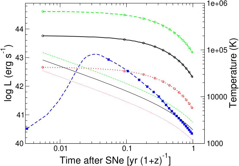
The magnitudes of primordial SNe are important as their occurrence rates to catch these events unfolding in the distant universe. We exploit the ⁵⁶Ni output from metal-free SNe models to calculate luminosities L(t) from the two-step decay of ⁵⁶Ni to ⁵⁶Fe (Heger & Woosley, 2002). We consider the emission spectrum to be a blackbody spectrum with a time-dependent temperature (20) calculated using free expansion arguments.

$$T(t)=\left[\frac{L(t)M}{8\pi\sigma Et^{2}}\right]^{1/4}(1+z),$$ (20)

where M is the stellar mass and E is the kinetic energy of the SNe. The temperature and luminosity of a 175, 200, and 250$M_{\odot}$ primordial star SNe are depicted in Figure 6. Kinetic energy is taken from the SNe models (Heger & Woosley, 2002).

In the upper range (M $>$ 200$M_{\odot}$) of pair-instability SNe, these events produce 1–57$M_{\odot}$ of ⁵⁶Ni (Heger & Woosley, 2002), which will produce tremendous luminosities compared to typical Type II SNe outputs of only 0.1–0.4 $M_{\odot}$ (Woosley & Weaver, 1986). However, uncertainty in the primordial IMF places doubt in the frequency of primordial star formation with high ⁵⁶Ni yields. Using conventional Type II SNe parameters of L $\simeq$ 3 $\times$ 10⁴² erg s^-1, T = 25000K (2 days $\,\buildrel<\over{\sim}\,$ t $\,\buildrel<\over{\sim}\,$ 7 days), and T = 7000K (7 days $\,\buildrel<\over{\sim}\,$ t $\,\buildrel<\over{\sim}\,$ 2 months) that are tuned by observed light curves, Miralda-Escudé & Rees (1997) determine apparent magnitudes that are 1–3 mag lower than our values, which is due to the greater nickel production of new pair-instability SNe models. Their model should apply to the pair-instability SNe with little ⁵⁶Ni ejecta. The temperatures are higher than our values because we allow for free expansion of the ejecta due to a lower external medium gas density. Radiation from the primordial star should expel most of surrounding medium to create a low density, highly ionized region of approximately 100 pc in size for a 120$M_{\odot}$ and 500$M_{\odot}$ primordial star, respectively (Whalen, Abel, & Norman, 2004).

In typical Type II light curves, radioactive decay does not significantly contribute to the luminosity in the plateau stage (Popov, 1993). In primordial SNe, the ⁵⁶Ni decay may overwhelm the typical sources of energy within the expanding fireball and create a totally different light curve. We stress that our light curve is a very rough estimate at the processes occurring within a primordial SNe.

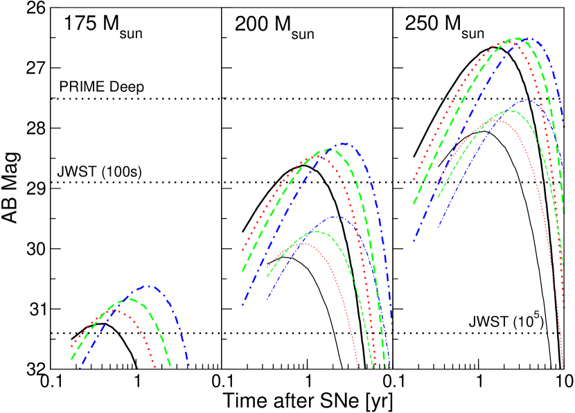
In Figure 7, we compare maximum AB magnitudes of low- and high-mass pair-instability SNe at various redshifts and sensitivities of space infrared observatories. We consider the sensitivities of SIRTF at 3.5µm, PRIME medium and deep surveys, and JWST with exposure times of 100s and 10⁵ s. We also give the typical light curve for a Supernova Type Ia. Clearly our simple estimate leads to very high predicted luminosities and more detailed numerical models of these explosions are clearly desirable.

Figure 8.— The solid line is the mean proper separation between minihalos. The dashed line is the redshift where minihalos first receive radiation from neighboring sources forming at the same epoch.

3.5. Other factors

Other factors could alter the feasibility of observing primordial SNe. For instance, $\sim$2% of primordial stars might die in collapsar gamma-ray bursts (GRBs) (Heger et al., 2002). Lamb (1999) also provides a ratio of GRBs to Type Ib/c SNe rates that is $\sim$3 $\times$ 10^-5 ($f_{beam}$ / 10^-2)^-1. However, this estimate is for a normal Salpeter IMF, and as mentioned before, the primordial star IMF could be skewed toward high masses, which would increase the probability of a GRB. Zero- and low-metallicity, massive stars outside the pair-instability mass range die as GRBs or jet-driven SNe, which are similar to GRBs but not as energetic and spectrally hard. If we consider a proportionality constant and beaming factor, we estimate that the all-sky primordial GRB rate,

$$R_{GRB}=2.8\left(\frac{\theta_{b}}{0.01}\right)\left(\frac{f_{GRB}}{0.02}\right)\;{\rm GRBs}\;{\rm yr}^{-1}.$$ (21)

In M $\,\buildrel<\over{\sim}\,$ 140$M_{\odot}$ stars, a collapsar results when it forms a proto-neutron stars, cannot launch a supernova shock, and directly collapses to form a black hole in $\sim$1 s (Woosley, 1993; MacFadyen & Woosley, 1999). In M $\,\buildrel>\over{\sim}\,$ 260$M_{\odot}$ stars, it does not create a proto-neutron star and directly collapses into a massive black hole (Fryer, Woosley, & Heger, 2001). Afterwards, these black holes can accrete gas and produce X-rays that can further ionize the Universe (Ricotti & Ostriker, 2004b). A few of these X-ray sources could be detected in the Chandra deep field (Ricotti, Ostriker, & Gnedin, 2004; Alexander et al., 2003). In most GRB models (for an overview, see Mészáros, 2002), the radiation is beamed to small opening angles due to relativistic effects, which would render a fraction of GRBs to be unobservable in our perspective. Finally, gravitational lensing will significantly increase the apparent magnitudes for selected primordial SNe for very small survey areas. However, the overall magnitude distribution is slightly dimmed by gravitational lensing (Marri & Ferrara, 1998; Marri, Ferrara, & Pozzetti, 2000).

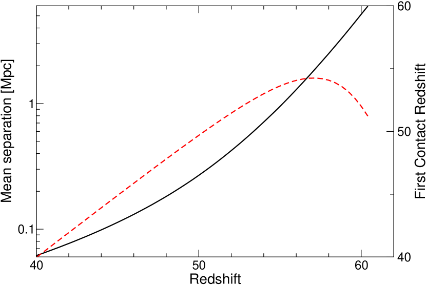
Using the proper minihalo density, we calculate the average light travel time between sources, which indicates when negative H₂ feedback first affects star formation. Star formation occurs $\sim$9.33 Myr after halo formation, so radiation escapes into the IGM at a time t_rad = t_H(z_form) + 9.33 Myr, where z_form is the halo formation redshift. These sources have a mean proper separation of d = $\rho_{\star}^{-1/3}$ / (1+z); therefore the time where radiation influences other halos is t_rad + d/c. The minimum of this time, corresponding to z = 54, is where radiation reaches other halos for the first time. The mean proper separation and epoch of first radiation effects are illustrated in Figure 8.

Deviations in the amplitudes of fluctuations, $\sigma_{8}$, and a running spectral model (Liddle & Lyth, 1992, 1993) also affect primodial SNe rates. We ran a set of models with $\sigma_{8}$ = 0.8, and predictably, the rates decreased by a factor of $\sim$2.5 due to lesser powers at small mass scales. When we match $\tau$ = 0.17, rates are 0.12–0.2 yr^-1 deg^-2 with the rates peaking earlier at z $\sim$ 20, but now the redshift peaks are nearly independent of redshift with only $\delta$z $\approx$ 1 separating the 100 and 500$M_{\odot}$ models. If we keep the protogalaxy parameters from the main models, rates do not change; however, the rates peak later than our main models by $\delta$z $\approx$ 4, and $\tau$ lowers to 0.14. According to inflationary models, the spectral index of flucutations should be slowly varying with scale. While analyzing WMAP data, Peiris et al. (2003) determined that the flucutation amplitude is significantly lower at small scales. With lesser powers at small scales, primordial SNe rates decrease such as the case of a lower $\sigma_{8}$. In principle, studying primordial SNe occurrences with respect to redshift could furnish direct constraints on the power spectrum at these small scales.

4. Constraining the Free Parameters

We have demonstrated our model’s dependence on the free parameters, $f_{esc}$, $f_{\star}$, and M_fs. We suggest several observational and numerical methods in order to constrain our models.

4.1. Observational

To constrain early star formation history of dwarf irregulars with the [$\alpha$/Fe] vs. [Fe/H] comparison, metal analyses of stars with [Fe/H] $<$ –1.5 are needed to determine early star formation rates of particular systems (See Figure 1.5 in Venn et al., 2003). Dwarf spheroidals exhibit greater variance in star formation histories from system to system, but a similar study will increase our knowledge of high redshift star formation in these small galaxies to further constrain $f_{\star}$ at high redshifts. To improve on these studies, the advances in multi-object spectrographs (e.g. VIMOS, FLAMES, and GMOS) enable the gathering of many stellar spectra in one exposure. This will greatly increase the stellar population data of dwarf galaxies.

Since some massive stars die as a long-duration GRB, these events can convey information from the death of both Pop II and III stars. The propagation of the initial burst and afterglow provide information about the total energy, gas density in the vicinity, and the Lorentz factor of the beam. The host galaxy ISM properties will help constrain the $f_{esc}$ in high redshift galaxies. As in the case of GRB 030329 (Stanek et al., 2003), the power-law spectra of the afterglow can be subtracted to obtain a residual that resembles a typical SN spectrum, which may be used to roughly determine the mass of the progenitor. Observing the afterglow is necessary to determine its redshift. The prospect of observing prompt afterglows will be accomplished easier with Swift, which can possibly detect GRB afterglows to z = 16 and 33 in the K and M bands, respectively (Gou et al., 2004). Furthermore, $\,\buildrel>\over{\sim}\,$50% of GRBs occur earlier than z = 5, and 15% of those high redshift GRBs are detectable by Swift (Bromm & Loeb, 2002). The comparison to nearby SNe can provide crucial information of the high redshift ISM. Finally, it is a possiblity to explore the intervening absorption with the fast-pointing and multi-wavelength observations of Swift (Vreeswijk, Møller, & Fynbo, 2003; Loeb, 2003; Barkana & Loeb, 2004). This IGM absorption would constrain the reionization history of the Universe better, which may change the primordial SNe rates, but more specifically the rate per unit redshift which would roughly conform to the filling factor evolution.

The radiation from protogalaxies and primordial stars will not only ionize the Universe but also contribute to the near-infrared background (NIRB). Calculations have shown that primordial stars can provide a significant fraction of radiation to the NIRB (Santos, Bromm, & Kamionkowski, 2002; Salvaterra & Ferrara, 2003); however, the paradigm of early reionization set by WMAP was not considered at the time. f_⋆ of protogalaxies and densities of primordial stars can be further constrained if future studies of the NIRB consider the large emissivities of zero- and low-metallicity sources at z $\,\buildrel>\over{\sim}\,$ 15.

Other outlooks include detecting high redshift radio sources and searching for 21cm absorption and emission (Hogan & Rees, 1979; Scott & Rees, 1990; Iliev et al., 2003; Furlanetto, Sokasian, & Hernquist, 2004). By looking for 21cm signatures, observations would be directly probing the neutral regions of the Universe since the Gunn-Peterson trough saturates only at a neutral filling factor of $\sim$10^-5. Lastly, additional searches for high redshift starbursts (e.g. Ellis et al., 2001; Pello et al., 2004) in lensed fields will furnish an understanding of the characteristics of these objects and help tighten our models of early “normal” and primordial star formation.

4.2. Numerical Simulations

Metal production from primordial stars cannot account for the volume filling factor of metals as seen in Ly$\alpha$ clouds in current models (Norman, O’Shea, & Paschos, 2004). Therefore, ubiquitous star formation in protogalaxies most likely polluted the sparse regions of the Universe. Combining the primordial and protogalaxy metal output, simulations with proper metal transport should agree with the abundances observed in Ly$\alpha$ clouds. Such simulations that takes into account both of these metal sources and matches the results of Songaila & Cowie (1996) and Songaila (2001) is needed to constrain star formation before reionization.

Numerical simulations are also needed to investigate radiative transfer from a protogalaxy stellar population. This scenario will contain more complexities than a single primordial star in a spherical halo as in Whalen, Abel, & Norman (2004). However a protogalactic simulation with the Jeans length resolved, star formation and feedback, and radiative transfer, it will be possible to study the evolution of the ISM in a protogalaxy, which will produce insight and better constraints on the photon escape fraction, $f_{esc}$, in the Lyman continuum at high redshifts. Ricotti, Gnedin, & Shull (2002a, b) thoroughly study radiative transfer around protogalaxies; however, $f_{esc}$ is still a parameter when it should be determined from the radiative transfer results in the simulations. Ideally, the analytical ideas about ionizing the Universe in Madau (1995); Haardt & Madau (1996); Madau, Haardt, & Rees (1999) should be realized in such simulations but in the context of the current paradigm of a high redshift reionization as indicated by WMAP. Also we may hope by using numerical radiative transfer techniques for line and continuum radiation in three dimension to push the simulations of Abel, Bryan, & Norman (2002) to follow the entire accretion phase of the first stars. This would lead to stronger constraints on the masses of the very first stars.

5. Summary and Conclusions

The WMAP measurement of optical depth to electron scattering places a constrain of early cosmological reionization of the universe, which we show to be mainly from star formation in protogalaxies. This general result is in agreement with other studies of reionization after WMAP (e.g. Cen, 2003a; Somerville & Livio, 2003; Ciardi, Ferrara, & White, 2003; Ricotti & Ostriker, 2004a; Sokasian et al., 2004).

• The radiation from protogalaxies squelches out primordial star formation, and $\sim$0.34 primordial SNe deg^-2 yr^-1 are expected. SNe rates can vary from 0.1 to $>$1.5 deg^-2 yr^-1 depending on the choice of primordial stellar mass and protogalaxy parameters while still constrained by the WMAP result. The peak of SNe rate occurs later with increasing primordial stellar masses. These results are upper limits since the rate of visible primordial SNe depends on the IMF because only a fraction will lie in the pair instability SNe mass range. The other massive primordial stars might result in jet-driven SNe or long duration GRBs.

• Stellar abundances and star formation in local dwarf galaxies aid in estimating protogalaxy characteristics. We choose f_⋆ = 0.04 and f_esc = 0.050 in our 100 $M_{\odot}$ model. In protogalaxies, the star formation efficiency is slightly lower than local values, but the photon escape fraction is within local observed fractions.

• Primordial stars enrich the IGM to a maximum volume-averaged [Fe/H] $\simeq$ –4.1 if the IMF is skewed toward the pair-instability upper mass range. A proper IMF will lessen this volume-averaged metallicity since only a fraction of stars will exist in this mass range. If complete metal mixing does not occur, there will be metal-rich and metal-poor regions relative to the universal metallicity.

• The entire error bar of the WMAP measurement of optical depth to electrons can be explained by a higher/lower f_⋆ and f_esc. Protogalaxies can ionize the IGM easily since low metallicity starburst models produce 20–80% more ionizing photons as previously used (Z = 0.001) IMFs. Massive primordial stars provide $\sim$10% of the necessary photons to achieve reionization. No exotic processes or objects are necessary.

• Only the upper mass range of pair instability SNe will be observable with JWST since the low mass counterparts do not produce enough ⁵⁶Ni to be very luminous.

Although the IMF of primordial stars is unknown, simulations have hinted that a fraction of metal-free stars may exist in the pair-instability mass range. When observational rates, light curves, and spectra are obtained from future surveys, these data would provide very stringent constraints on the underlying CDM theory as well as our understanding of primordial star formation.

References

- Abel et al. (1998) Abel, T., Anninos, P., Norman, M. L., & Zhang, Y. 1998, ApJ, 508, 518
- Abel, Bryan, & Norman (2000) Abel, T., Bryan, G. L., & Norman, M. L. 2000, ApJ, 540, 39
- Abel, Bryan, & Norman (2002) Abel, T., Bryan, G. L., & Norman, M. L. 2002, Science, 295, 93
- Alexander et al. (2003) Alexander, D. M., et al. 2003, AJ, 126, 539
- Bardeen et al. (1986) Bardeen, J. M., Bond, J. R., Kaiser, N., & Szalay, A. S. 1986, ApJ, 304, 15
- Barkana & Loeb (2004) Barkana, R. & Loeb, A. 2004, ApJ, 601, 64
- Barkat, Rakavy, & Sack (1967) Barkat, Z, Rakavy, G., & Sack, N. 1967, Phys. Rev. Lett., 18, 379
- Becker et al. (2002) Becker, R. H. et al. 2001, AJ, 122, 2850
- Bond, Arnett, & Carr (1984) Bond, J. R., Arnett, W. D., & Carr, B. J. 1984, ApJ, 280, 825
- Bromm, Coppi, & Larson (2002) Bromm, V., Coppi, P. S., & Larson, R. B. 2002, ApJ, 564, 23
- Bromm & Loeb (2002) Bromm, V. & Loeb, A. 2002, ApJ, 575, 111
- Bryan & Norman (1999) Bryan, G. L. & Norman, M. L. 1999, in Workshop on Structured Adaptive Mesh Refinement Grid Methods, IMA Volumes in Mathematics 117, ed. N. Chrisochoides (New York: Springer), 165
- Cen (2003a) Cen, R. 2003a, ApJ, 591, L5
- Cen (2003b) Cen, R. 2003b, ApJ, 591, 12
- Christlieb et al. (2002) Christlieb, N. et al. 2002, Nature, 419, 904
- Ciardi, Ferrara, & White (2003) Ciardi, B., Ferrara, A., & White, S. D. M. 2003, MNRAS, 344, L7
- Couchman & Rees (1986) Couchman, H. M. P. & Rees, M. J. 1986, MNRAS, 221, 53
- Cowie et al. (1995) Cowie, L. L., Songaila, A., Kim, T., & Hu, E. M. 1995, AJ, 109, 1522
- Dekel & Rees (1987) Dekel, A., & Rees, M. J. 1987, Nature, 326, 455
- Ellis et al. (2001) Ellis, R., Santos, M. R., Kneib, J., & Kuijken, K. 2001, ApJ, 560, L119
- Miralda-Escudé (2003) Miralda-Escudé, J. 2003, Science, 300, 1904
- Fan et al. (2002) Fan, X., Narayanan, V. K., Strauss, M. A., White, R. L., Becker, R. H., Pentericci, L., & Rix, H. 2002, AJ, 123, 1247
- Field, Somerville, & Dressler (1966) Field, G. B., Somerville, W. B., & Dressler, K. 1966, ARA&A, 4, 207
- Fryer (1999) Fryer, C. L. 1999, ApJ, 522, 413
- Fryer, Woosley, & Heger (2001) Fryer, C. L., Woosley, S. E., & Heger, A. 2001, ApJ, 550, 372
- Fuller & Couchman (2001) Fuller, T. M. & Couchman, H. M. P. 2000, ApJ, 544, 6
- Furlanetto, Sokasian, & Hernquist (2004) Furlanetto, S. R., Sokasian, A., & Hernquist, L. 2004, MNRAS, 347, 187
- Gnedin (2000) Gnedin, N. Y. 2000, ApJ, 535, L75
- Gou et al. (2004) Gou, L. J., Mészáros, P., Abel, T., & Zhang, B. 2004, ApJ, 604, 508
- Haardt & Madau (1996) Haardt, F. & Madau, P. 1996, ApJ, 461, 20
- Haehnelt (1995) Haehnelt, M. G. 1995, MNRAS, 273, 249
- Haiman, Abel, & Madau (2001) Haiman, Z., Abel, T., & Madau, P. 2001, ApJ, 551, 599
- Haiman, Abel, & Rees (2000) Haiman, Z., Abel, T., & Rees, M. J. 2000, ApJ, 534, 11
- Haiman & Loeb (1997) Haiman, Z. & Loeb, A. 1997, ApJ, 483, 21
- Haiman, Rees, & Loeb (1997) Haiman, Z., Rees, M. J., & Loeb, A. 1997, ApJ, 476, 458
- Heckman et al. (2001) Heckman, T. M., Sembach, K. R., Meurer, G. R., Leitherer, C., Calzetti, D., & Martin, C. L. 2001, ApJ, 558, 56
- Heger et al. (2002) Heger, A., Fryer, C. L., Woosley, S. E., Langer, N., & Hartmann, D. H. 2003, ApJ, 591, 288
- Heger & Woosley (2002) Heger, A. & Woosley, S. E. 2002, ApJ, 567, 532
- Hogan & Rees (1979) Hogan, C. J. & Rees, M. J. 1979, MNRAS, 188, 791
- Hui & Haiman (2003) Hui, L. & Haiman, Z. 2003, ApJ, 596, 9
- Hurwitz, Jelinsky, & Dixon (1997) Hurwitz, M., Jelinsky, P., & Dixon, W. V. D. 1997, ApJ, 481, L31
- Iliev et al. (2003) Iliev, I. T., Scannapieco, E., Martel, H., & Shapiro, P. R. 2003, MNRAS, 341, 81
- Kauffmann et al. (2003) Kauffmann, G. et al. 2003, MNRAS, 341, 33
- Kim et al. (1997) Kim, T., Hu, E. M., Cowie, L. L., & Songaila, A. 1997, AJ, 114, 1
- Kogut et al. (2003) Kogut, A., et al. 2003, ApJS, 148, 161
- Lamb (1999) Lamb, D. Q. 1999, A&AS, 138, 607
- Leitherer et al. (1995) Leitherer, C., Ferguson, H. C., Heckman, T. M., & Lowenthal, J. D. 1995, ApJ, 454, L19
- Leitherer et al. (1999) Leitherer, C. et al. 1999, ApJS, 123, 3
- Liddle & Lyth (1992) Liddle, A. R. & Lyth, D. H. 1992, Phys. Lett. B, 291, 391
- Liddle & Lyth (1993) Liddle, A. R. & Lyth, D. H. 1993, Phys. Rep., 231, 1
- Loeb (2003) Loeb, A. 2003, Proc. of IAU Colloquium 192 on “Supernovae”, April 2003, Valencia, Spain, eds. J. M. Marcaide and K. W. Weiler (astro-ph/0307231)
- Loeb & Barkana (2001) Loeb, A. & Barkana, R. 2001, ARA&A, 39, 19
- MacFadyen & Woosley (1999) MacFadyen, A. I. & Woosley, S. E. 1999, ApJ, 524, 262
- Machacek, Bryan, & Abel (2001) Machacek, M. E., Bryan, G. L., & Abel, T. 2001, ApJ, 548, 509
- Madau (1995) Madau, P. 1995, ApJ, 441, 18
- Madau, Haardt, & Rees (1999) Madau, P., Haardt, F., & Rees, M. J. 1999, ApJ, 514, 648
- Maeder (1992) Maeder, A. 1992, A&A, 264, 105
- Marri & Ferrara (1998) Marri, S. & Ferrara, A. 1998, ApJ, 509, 43
- Marri, Ferrara, & Pozzetti (2000) Marri, S., Ferrara, A., & Pozzetti, L. 2000, MNRAS, 317, 265
- Mateo (1998) Mateo, M. L. 1998, ARA&A, 36, 435
- Matteucci (2002) Matteucci, F. 2002, in Proceedings of The Evolution of Galaxies III (astro-ph/0210540)
- Matteucci & Recchi (2001) Matteucci, F. & Recchi, S. 2001, ApJ, 558, 351
- Mészáros (2002) Mészáros, P. 2002, ARA&A, 40, 137
- Miralda-Escudé & Rees (1997) Miralda-Escudé, J. & Rees, M. J. 1997, ApJ, 478, L57
- Mo & White (2002) Mo, H. J. & White, S. D. M. 2002, MNRAS, 336, 112
- Norman, O’Shea, & Paschos (2004) Norman, M. L., O’Shea, B. W., & Paschos, P. 2004, ApJ, 601, L115
- Norris, Ryan, & Beers (2001) Norris, J. E., Ryan, S. G., & Beers, T. C. 2001, ApJ, 561, 1034
- Oh & Haiman (2003) Oh, S. P. & Haiman, Z. 2003, MNRAS, 346, 456
- Peebles (1993) Peebles, P. J. E. 1993, Principles of Physical Cosmology (Princeton: Princeton University Press)
- Peiris et al. (2003) Peiris, H. V., et al. 2003, ApJS, 148, 213
- Pello et al. (2004) Pelló, R., Schaerer, D., Richard, J., Le Borgne, J.-F., & Kneib, J.-P. 2004, A&A, 416, L35
- Popov (1993) Popov, D. V. 1993, ApJ, 414, 712
- Press & Schechter (1974) Press, W. H. & Schechter, P. 1974, ApJ, 187, 425
- Qian & Wasserburg (2002) Qian, Y.-Z. & Wasserburg, G. J. 2002, ApJ, 567, 515
- Rauch et al. (1997) Rauch, M., Haehnelt, M. G., & Steinmetz, M. 1997, ApJ, 481, 601
- Rauscher et al. (2002) Rauscher, T., Heger, A., Hoffman, R. D., & Woosley, S. E. 2002, ApJ, 576, 323
- Renzini & Voli (1981) Renzini, A. & Voli, M. 1981, A&A, 94, 175
- Ricotti, Gnedin, & Shull (2002a) Ricotti, M., Gnedin, N. Y., & Shull, J. M. 2002a, ApJ, 575, 49
- Ricotti, Gnedin, & Shull (2002b) Ricotti, M., Gnedin, N. Y., & Shull, J. M. 2002b, ApJ, 575, 33
- Ricotti & Ostriker (2004a) Ricotti, M. & Ostriker, J. P. 2004, MNRAS, 350, 539
- Ricotti & Ostriker (2004b) Ricotti, M. & Ostriker, J. P. 2004, MNRAS, 352, 547
- Ricotti, Ostriker, & Gnedin (2004) Ricotti, M., Ostriker, J. P., & Gnedin, N. Y. 2004, MNRAS, submitted (astro-ph/0404318)
- Ricotti & Shull (2000) Ricotti, M. & Shull, J. M. 2000, ApJ, 542, 548
- Salvaterra & Ferrara (2003) Salvaterra, R. & Ferrara, A. 2003, MNRAS, 339, 973
- Santos, Bromm, & Kamionkowski (2002) Santos, M. R., Bromm, V., & Kamionkowski, M. 2002, MNRAS, 336, 1082
- Schaerer (2000) Schaerer, D. 2000, ASP Conf. Ser. 221: Stars, Gas and Dust in Galaxies: Exploring the Links, 99
- Schaerer (2002) Schaerer, D. 2002, A&A, 382, 28
- Schaerer (2003) Schaerer, D. 2003, A&A, 397, 527
- Scott & Rees (1990) Scott, D. & Rees, M. J. 1990, MNRAS, 247, 510
- Sheth, Mo, & Tormen (2001) Sheth, R. K., Mo, H. J., & Tormen, G. 2001, MNRAS, 323, 1
- Sheth & Tormen (1999) Sheth, R. K. & Tormen, G. 1999, MNRAS, 308, 119
- Sheth & Tormen (2002) Sheth, R. K. & Tormen, G. 2002, MNRAS, 329, 61
- Smith, Norris, & Crowther (2002) Smith, L. J., Norris, R. P. F., & Crowther, P. A. 2002, MNRAS, 337, 1309
- Sokasian et al. (2004) Sokasian, A., Yoshida, N., Abel, T., Hernquist, L., & Springel, V. 2004, MNRAS, 350, 47
- Somerville & Livio (2003) Somerville, R. S. & Livio, M. 2003, ApJ, 593, 611
- Songaila & Cowie (1996) Songaila, A. & Cowie, L. L. 1996, AJ, 112, 335
- Songaila (2001) Songaila, A. 2001, ApJ, 561, L153
- Stanek et al. (2003) Stanek, K. Z., et al. 2003, ApJ, 591, L17
- Stecher & Williams (1967) Stetcher, T. P. & Williams, D. A. 1967, ApJ, 149, 29
- Steidel, Pettini, & Adelberger (2001) Steidel, C. C., Pettini, M., & Adelberger, K. L. 2001, ApJ, 546, 665
- Taylor et al. (1999) Taylor, C. L., Hüttemeister, S., Klein, U., & Greve, A. 1999, A&A, 349, 424
- Tegmark et al. (1997) Tegmark, M., Silk, J., Rees, M. J., Blanchard, A., Abel, T., & Palla, F. 1997, ApJ, 474, 1
- Venn et al. (2003) Venn, K., Tolstoy, E., Kaufer, A., & Kudritzki, R. P. 2003, Carnegie Obs. Astrophy. Series, Vol. 4, Origin and Evolution of the Elements (astro-ph/0305188)
- Vreeswijk, Møller, & Fynbo (2003) Vreeswijk, P. M., Møller, P., & Fynbo, J. P. U. 2003, A&A, 409, L5
- Walter et al. (2001) Walter, F., Taylor, C. L., Hüttemeister, S., Scoville, N. & McIntyre, V. 2001, AJ, 121, 727
- Whalen, Abel, & Norman (2004) Whalen, D., Abel, T. & Norman, M. L. 2004, ApJ, 610, 14
- Wood & Loeb (2000) Wood, K. & Loeb, A. 2000, ApJ, 545, 86
- Woosley (1993) Woosley, S. E. 1993, ApJ, 405, 273
- Woosley & Weaver (1986) Woosley, S. E. & Weaver, T. A. 1986, ARA&A, 24, 205
- York et al. (2000) York, D. G. et al. 2000, AJ, 120, 1579
- Zheng et al. (2003) Zheng, W., et al. 2003, Proc. SPIE, 4850, 1132