The Intermediate-scale Clustering of Luminous Red Galaxies

Abstract

We report the intermediate-scale ($0.3$ to $40h^{-1}{\rm\,Mpc}$) clustering of $35,000$ luminous early-type galaxies at redshifts $0.16$ to $0.44$ from the Sloan Digital Sky Survey. We present the redshift-space two-point correlation function $\xi(s)$, the projected correlation function ${w_{p}(r_{p})}$, and the deprojected real-space correlation function $\xi(r)$, for approximately volume-limited samples. As expected, the galaxies are highly clustered, with the correlation length varying from $9.8\pm 0.2h^{-1}{\rm\,Mpc}$ to $11.2\pm 0.2h^{-1}{\rm\,Mpc}$, dependent on the specific luminosity range. For the $-23.2<M_{g}<-21.2$ sample, the inferred bias relative to that of $L_{*}$ galaxies is $1.84\pm 0.11$ for $1h^{-1}{\rm\,Mpc}<r_{p}\lesssim 10h^{-1}{\rm\,Mpc}$, with yet stronger clustering on smaller scales. We detect luminosity-dependent bias within the sample but see no evidence for redshift evolution between $z=0.2$ and $z=0.4$. We find a clear indication for deviations from a power-law in the real-space correlation function, with a dip at $\sim\!2h^{-1}{\rm\,Mpc}$ scales and an upturn on smaller scales. The precision measurements of these clustering trends offer new avenues for the study of the formation and evolution of these massive galaxies.

1 Introduction

The clustering of galaxies provides a window not only to the formation of inhomogeneities in the early universe but also onto the physics of galaxy formation. Galaxies with different properties cluster differently (Hubble, 1936; Zwicky et al., 1968; Davis & Geller, 1976; Dressler, 1980; Postman & Geller, 1984; Hamilton, 1988; White, Tully, & Davis, 1988; Park et al., 1994; Loveday et al., 1995; Guzzo et al., 1997; Benoist et al., 1996; Willmer, da Costa & Pellegrini, 1998; Brown, Webster & Boyle, 2000; Carlberg et al., 2001; Norberg et al., 2001; Zehavi et al., 2002; Norberg et al., 2002; Budavari et al., 2003; Madgwick et al., 2003; Hogg et al., 2003; Zehavi et al., 2004b), and these trends can be connected to their small-scale environments, notably the masses of their host dark matter halos (e.g., Kaiser 1984; Bardeen et al. 1986; Mo & White 1996; Benson et al. 2000; Sheth, Mo, & Tormen 2001; Berlind et al. 2003). This path has been strengthened recently by the discovery of deviations from the canonical power-law correlation function on small scales (e.g., Zehavi et al. 2004a; Zheng 2004) and the ease of interpretation of these features by contemporary models of galaxy and halo clustering, in terms of the clustering of galaxies within single halos and the clustering between halos (Kauffmann, Nusser, & Steinmetz, 1997; Jing, Mo, & Börner, 1998; Kauffman et al., 1999; Benson et al., 2000; Ma & Fry, 2000; Peacock & Smith, 2000; Seljak, 2000; Scoccimarro et al., 2001; Berlind & Weinberg, 2002; Berlind et al., 2003; Magliocchetti & Porciani, 2003; Kravtsov et al., 2004; Zehavi et al., 2004a; Zheng, 2004).

The Sloan Digital Sky Survey (SDSS;York et al. 2000) was designed in scope and systematic control to permit the study of galaxy clustering over a wide range of scales and galaxy properties (e.g., Connolly et al. 2002; Zehavi et al. 2002; Budavari et al. 2003; Hogg et al. 2003; Tegmark et al. 2004; Zehavi et al. 2004b; all using the SDSS main galaxy sample). To improve the precision of clustering measurements on the largest scales, the SDSS provides a spectroscopic sample of luminous red galaxies (LRG). These galaxies reach a redshift of 0.5, thereby providing a sample of over $1h^{-3}{\rm\,Gpc^{3}}$ (see Eisenstein et al. 2001). Thus far, over 50,000 spectra of LRGs have been acquired.

In this paper, we will investigate the clustering of these luminous early-type galaxies on scales between $0.3$ and $40h^{-1}{\rm\,Mpc}$. This stretches from the quasi-linear to the deeply non-linear regime. As massive early-type galaxies are known to inhabit preferentially rich environments (e.g., Sandage 1972; Dressler 1980; Hoessel et al. 1980; Schneider et al. 1983; Postman & Geller 1984; Postman & Lauer 1995,M. Bernardi 2004, in preparation), this selection should permit one to study the clustering and internal structure of massive halos. Models that differ in their association of LRGs to cluster-sized halos or to the fraction in smaller halos will vary not only in their predicted correlation length, but also in the fine structure of the correlation functions. With the sample size available within the SDSS LRG sample, we expect to reach the precision necessary to perform such tests despite the rarity of massive galaxies. We note that the rapid increase in the clustering of early-type galaxies at the highest luminosities (Hogg et al., 2003; Zehavi et al., 2004b) implies that the connections between the most massive galaxies and their environments is notably different than even $L_{*}$ early-types.

The outline of the paper is as follows. In § 2 we present the LRG sample. In § 3 we present the clustering measurements in redshift-space and in § 4 we show the inferred real-space clustering results. We conclude in § 5. Details of our sample modeling are given in the Appendix.

Throughout the paper, all distances are comoving and quoted in $h^{-1}{\rm\,Mpc}$, where $h\equiv H_{0}/100{\rm\ km\ s^{-1}\ Mpc^{-1}}$. For all distances and absolute magnitude we use a cosmology of $\Omega_{m}=0.3$ and $\Lambda=0.7$ and adopt $h=1$ to compute absolute magnitudes.

2 Data

2.1 The SDSS LRG Sample

The SDSS (York et al., 2000) is imaging $10^{4}$ square degrees away from the Galactic Plane in 5 passbands, $u$, $g$, $r$, $i$, and $z$ (Fukugita et al., 1996; Gunn et al., 1998). Image processing (Lupton et al., 2001; Stoughton et al., 2002; Pier et al., 2003) and calibration (Hogg et al., 2001; Smith et al., 2002) allow one to select galaxies, quasars, and stars for follow-up spectroscopy with twin fiber-fed double-spectrographs. The spectra cover 3800Å to 9200Å with a resolution of 1800. Targets are assigned to plug plates with a tiling algorithm that ensures nearly complete samples (Blanton et al., 2003a). An operational constraint of using fibers to obtain spectra is that no two fibers can be closer than $55^{\prime\prime}$ on the same plate. This constraint is partly alleviated by having roughly a third of the sky covered by overlapping plates.

Galaxy spectroscopic target selection proceeds by two algorithms. The primary sample (Strauss et al., 2002), referred to here as the MAIN sample, targets galaxies brighter than $r<17.77$. The surface density of such galaxies is about 90 per square degree. The LRG algorithm (Eisenstein et al., 2001) then selects $\sim\!12$ additional galaxies per square degree, using color-magnitude cuts in $g$, $r$, and $i$ to select galaxies to $r<19.5$ that are likely to be luminous early-types at redshifts up to $\sim\!0.5$. The selection is extremely efficient, and the redshift success rate is very high. A few galaxies (3 per square degree at $z>0.15$) matching the rest-frame color and luminosity properties of the LRGs are extracted from the MAIN sample; we refer to this combined set as the LRG sample. In detail, there are two parts to the LRG algorithm, known as Cut I and Cut II and described in Eisenstein et al. (2001).

We begin from a spectroscopic sample covering 3,836 square degrees. The exact survey geometry is expressed in terms of spherical polygons and is known as lss_sample14 (M. Blanton 2004, in preparation). This set contains 55,000 spectroscopic LRGs in the redshift range $0.15<z<0.55$.

2.2 Redshift and Magnitude Cuts

The SDSS LRG sample is nearly volume-limited, but not precisely so. At $z>0.37$, the flux limits of $r<19.2$ (Cut I) and $r<19.5$ (Cut II) begin to move into the passively-evolving luminosity threshold. In this paper, we wish to analyze volume-limited samples, so as to study the clustering properties of well defined populations of galaxies. We therefore define three subsamples in passively-evolved luminosity and restrict the redshift ranges to ensure complete coverage. The subsamples are $-23.2<M_{g}<-21.2$ with $0.16<z<0.36$, $-23.2<M_{g}<-21.8$ with $0.16<z<0.44$, and $-22.6<M_{g}<-21.6$ with $0.16<z<0.36$. The first of these sets is picked to maximize our use of the LRG spectroscopy for the innately volume-limited portion of the sample. The second is selected because the Cut II selection creates a knee in the number densities as a function of redshift that we can exploit. The third is chosen to match the luminosity range of the $-23<M_{r}<-22$ volume-limited MAIN galaxy sample described in Zehavi et al. (2004b). We use here only the red subsample of the latter (as defined in Zehavi et al. 2004b, with $0.10<z<0.23$) to compare to the LRG clustering. These LRG and MAIN samples overlap nearly completely in the redshift range in common, $0.16<z<0.23$. The basic information regarding the three LRG samples is summarized in Table 1, and their comoving number density as a function of redshift is shown in Figures 1-3.

Table 1:

LRG Sample Statistics
$M_{g}$ Redshift Number Density $\left<M_{g}\right>$ $\left<z\right>$ $-23.2<M_{g}<-21.2$ $0.16<z<0.36$ 29298 $9.7\times 10^{-5}$ -21.63 0.28 $-23.2<M_{g}<-21.8$ $0.16<z<0.44$ 12992 $2.4\times 10^{-5}$ -22.01 0.34 $-22.6<M_{g}<-21.6$ $0.16<z<0.36$ 14500 $4.8\times 10^{-5}$ -21.84 0.28

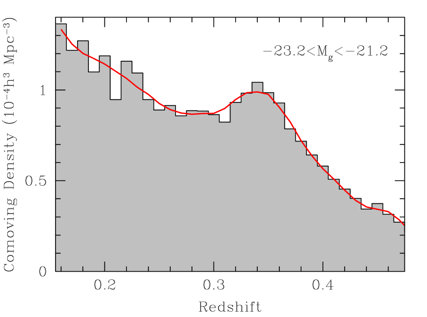
Figure 1: The comoving number density of the $-23.2<M_{g}<-21.2$ sample. The shaded histogram is the distribution of the actual data, and the solid continuous line is our model for the redshift distribution, described in Appendix A. The sample is close to a constant comoving volume for $z<0.36$, although the fluctuations are reaching about 30% peak-to-peak (but one should note that the lowest redshifts, where the excess is, contain less volume than the redshift range would suggest).

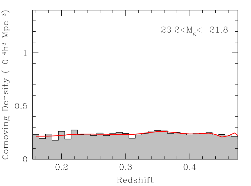
Figure 2: As Figure 1, but for the $-23.2<M_{g}<-21.8$ sample. The sample is close to a constant comoving volume for $z<0.44$.

Figure 3: As Figure 1, but for the $-22.6<M_{g}<-21.6$ sample. The sample is close to a constant comoving volume for $z<0.36$.

The above luminosities have been $k$-corrected and passively evolved to rest-frame magnitudes at $z=0.3$ (near the median redshift of the LRG sample). We use the observed $r$-band to estimate rest-frame $g$, as this requires minimal $k$-corrections at $z=0.3$. We have used the “non-star-forming” model presented in Appendix B of Eisenstein et al. (2001) but normalized to $M_{g}$ at $z=0.3$. The model has relatively mild evolution, only about 1 magnitude per unit redshift, compared to other measurements (Blanton et al., 2003b). Additional details of the samples’ modeling are given in Appendix A. To the extent that our model is appropriate, our selections represent mass thresholds throughout the sample volume. However, as shown in Figure 1, the $-23.2<M_{g}<-21.2$ sample still has some redshift evolution in the number density. This is due to small fluctuations in the selection thresholds of the parent sample in luminosity and rest-frame color as a function of redshift. The other two samples, being safely more luminous than the LRG sample selection limits, are much closer to a constant comoving threshold (Figs. 2 and 3).

3 Redshift-Space Clustering

We calculate the LRG correlation function in redshift space as a function of the redshift-space separation $s$. To estimate the mean density and account for the complex survey geometry, we generate random catalogs, applying the radial and angular selection functions of the samples. The details of the radial and angular modeling are given in the Appendix. We typically use in each random catalog 100-150 times the number of galaxies in the real sample, and we have verified that changing the random catalog makes negligible difference to the results. We estimate the correlation function using the Landy & Szalay (1993) estimator

$$\xi=\frac{DD-2DR+RR}{RR},$$ (1)

where DD, DR and RR are the suitably normalized numbers of weighted data-data, data-random and random-random pairs in each separation bin. We weight the galaxies (real and random) according to the angular and radial selection functions. We use a simple weighting by the inverse of the selection function, as the samples we use are all approximately volume-limited, and we have verified that our results are insensitive to employing alternative weighting schemes. We also used the alternative $\xi$ estimators of Davis & Peebles (1983) and Hamilton (1993) and found no significant differences in the results.

Here, and throughout the paper, we estimate statistical errors on our measurements using jackknife resampling with 104 angular subsamples. Each subsample excludes roughly 37 square degrees (generally contiguous on the sky), which is about $90h^{-1}{\rm\,Mpc}$ comoving on a side at $z=0.3$. The 2.5 degree SDSS stripes are $36h^{-1}{\rm\,Mpc}$ comoving at $z=0.3$. Zehavi et al. (2004b) performed extensive tests with mock catalogs to check the reliability of the jackknife error estimates over a similar range of separations (see their Fig. 2). Their tests showed that the jackknife method is a robust way to estimate the error covariance matrix, especially for large volumes as probed here.

Figure 4 shows the redshift-space correlation function, $\xi(s)$, for the $-23.2<M_{g}<-21.2$ and $-23.2<M_{g}<-21.8$ LRG samples introduced in § 2.2, with errorbars obtained from the jackknife resampling. The small difference in amplitude arises from the difference in the average luminosity of the galaxies in the samples (see Table 1), reflecting the known trend of stronger clustering with luminosity (e.g., Hamilton 1988; Park et al. 1994; Loveday et al. 1995; Benoist et al. 1996; Guzzo et al. 1997; Norberg et al. 2001; Zehavi et al. 2002; Hogg et al. 2003; Zehavi et al. 2004b). The redshift-space correlation functions values are given in Table 2.

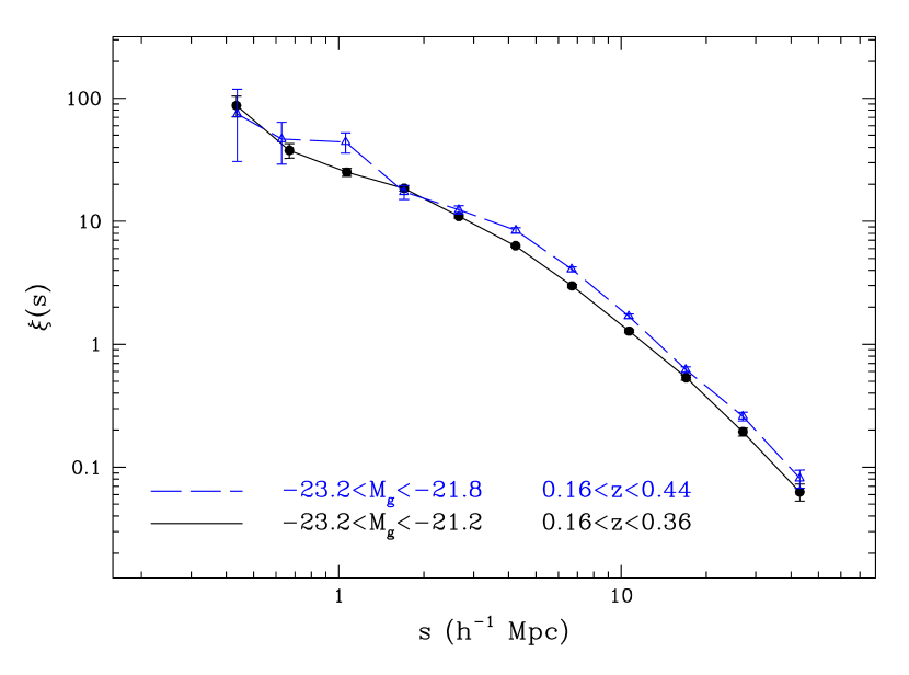
Figure 4: Redshift-space correlation function $\xi(s)$ for the LRG samples. Bins in $s$ are in logarithmic separation of $0.2$.

Table 2:

Correlation Functions Measurements
$-23.2<M_{g}<-21.2$ $-23.2<M_{g}<-21.8$ $-22.6<M_{g}<-21.6$ separation $\xi(s)$ ${w_{p}(r_{p})}$ $\xi(r)$ $\xi(s)$ ${w_{p}(r_{p})}$ $\xi(r)$ $\xi(s)$ ${w_{p}(r_{p})}$ $\xi(r)$ 0.418 87.4 (16.8) 772.9 (52.7) 675.7 (80.6) 74.6 (44.0) 1281 (243) 1276 (399) 39.6 (17.7) 743.9 (86.8) 484 (133) 0.663 37.7 (5.1) 414.4 (26.0) 210.3 (23.3) 46.6 (17.5) 575.2 (86.9) 332.8 (84.8) 30.3 (8.9) 548.0 (66.8) 316.9 (59.7) 1.051 25.1 (1.9) 238.8 (13.4) 66.9 (7.9) 44.2 (8.3) 286.8 (33.8) 83.1 (21.8) 30.9 (4.3) 268.0 (29.0) 75.5 (16.7) 1.665 18.5 (0.9) 154.9 (7.5) 24.9 (3.0) 17.3 (2.3) 178.5 (20.6) 26.0 (7.8) 19.4 (1.8) 174.6 (14.1) 30.8 (5.4) 2.639 11.0 (0.3) 109.0 (5.1) 11.7 (1.0) 12.4 (1.0) 132.4 (12.6) 13.0 (3.2) 12.1 (0.8) 111.6 (9.0) 10.1 (2.1) 4.182 6.32 (0.15) 74.0 (3.8) 5.04 (0.47) 8.45 (0.45) 95.5 (7.8) 6.01 (1.11) 7.35 (0.33) 84.9 (7.1) 5.58 (0.88) 6.628 2.99 (0.08) 50.5 (2.6) 2.32 (0.19) 4.08 (0.19) 70.8 (4.8) 3.80 (0.50) 3.52 (0.14) 59.2 (4.1) 2.62 (0.34) 10.505 1.28 (0.04) 33.0 (2.2) 1.04 (0.09) 1.70 (0.08) 38.8 (3.6) 1.16 (0.19) 1.52 (0.06) 40.1 (3.1) 1.25 (0.16) 16.650 0.54 (0.03) 20.0 (1.8) 0.43 (0.05) 0.62 (0.03) 25.2 (2.2) 0.56 (0.09) 0.59 (0.04) 25.1 (2.5) 0.57 (0.08) 26.388 0.19 (0.02) 11.0 (1.4) 0.14 (0.02) 0.26 (0.02) 13.2 (2.0) 0.17 (0.06) 0.23 (0.02) 13.2 (1.8) 0.20 (0.05)

NOTES.—Measurements of the redshift-space correlation function, $\xi(s)$, projected correlation function, ${w_{p}(r_{p})}$, and real-space correlation function, $\xi(r)$, for the three LRG samples discussed in the paper. Correlation functions are calculated for each sample over the range for which it is approximately volume-limited, denoted in Table 1. Comoving separations and ${w_{p}(r_{p})}$ values are in $h^{-1}{\rm\,Mpc}$ units. Redshift-space $\xi(s)$ and real-space $\xi(r)$ are dimensionless. The diagonal terms of the measurements error covariance matrices are given in parentheses. Our radial bins are logarithmically spaced with widths of 0.2 dex beginning at $10^{-0.49}$. The separations listed in column 1 are the linear centers of the bins. Strictly speaking, the listed values of $\xi(s)$ and $w_{p}(r_{p})$ are the averages of these correlation functions over the annuli. However, for reasonable power-law interpolations, the values of $w_{p}(r_{p})$ and $\xi(r)$ are very nearly ($\ll 1\%$) the values at the linear bin centers. The interpolated value of $\xi(s)$ at the bin centers would be about $1.5\%$ higher than the values in the table.

Figure 5 shows $\xi(s)$ for the $-22.6<M_{g}<-21.6$ LRG sample plotted together with $\xi(s)$ obtained for the comparable red $-23<M_{r}<-22$ MAIN galaxy subsample of Zehavi et al. (2004b), where we restrict the LRG sample to $0.23<z<0.36$, such that we are probing independent volumes. The LRG sample contains $\sim\!12400$ galaxies, while the MAIN galaxy sample includes only $\sim\!2700$. As is obvious from the plot, the agreement between the samples is excellent, and the LRG results thus extend in essence the MAIN galaxy clustering results to higher redshifts. The deviations at small separations are mainly due to shot noise effects arising from the small number of galaxies in the MAIN sample and are consistent within the errorbars. The numerical values of this LRG correlation function are also provided in Table 2.

Figure 5: Redshift-space correlation function $\xi(s)$ for the $-22.6<M_{g}<-21.6$ passively-evolved LRG sample and the comparable one from the MAIN galaxy sample.

4 Real-Space Clustering

4.1 Projected Correlation Function

To separate effects of redshift distortions from spatial correlations, it is customary to estimate the correlation function on a two dimensional grid of pair separations parallel ($\pi$) and perpendicular ($r_{p}$) to the line of sight, termed $\xi(r_{p},\pi)$. One can then learn about the real-space correlation function by computing the projected correlation function

$${w_{p}(r_{p})}=2\int_{0}^{\infty}d\pi\,\xi(r_{p},\pi).$$ (2)

In practice, we integrate up to $\pi_{max}=80h^{-1}{\rm\,Mpc}$, which is large enough to include most correlated pairs and gives a stable result. The omission of pairs at $\pi>80h^{-1}{\rm\,Mpc}$ likely causes an overestimate of $w_{p}(r_{p})$ by 1–$2h^{-1}{\rm\,Mpc}$, as the correlations on such scales are driven negative by redshift distortions. However, we have varied $\pi_{max}$ from 50–120$h^{-1}{\rm\,Mpc}$ without significant change in $w_{p}$. We also checked the robustness to binning in $r_{p}$ and in the integrated-over $\pi$ direction, finding the results to be insensitive to either.

The projected correlation function can in turn be related to the real-space correlation function, $\xi(r)$,

$${w_{p}(r_{p})}=2\int_{r_{p}}^{\infty}rdr\;\xi(r)(r^{2}-{r_{p}}^{2})^{-1/2}$$ (3)

(Davis & Peebles, 1983). In particular, fitting a power-law to the ${w_{p}(r_{p})}$ measurement allows us to infer the best-fit power law for $\xi(r)$.

Figure 6 shows the resulting projected correlation function, ${w_{p}(r_{p})}$, for the two inclusive LRG samples analyzed in this paper. Again, the differences in amplitude reflect the luminosity bias between the samples.

Figure 6: Projected correlation function ${w_{p}(r_{p})}$ for the LRG samples.

Figure 7 shows the normalized (such that the diagonal is 1) jackknife error covariance matrix of the ${w_{p}(r_{p})}$ measurements for the $-23.2<M_{g}<-21.2$ sample. As is apparent, there is significant correlation between the measurements on different scales, but the auto-correlation along the diagonal is relatively strong with the cross-correlation falling off rapidly.

Figure 7: Normalized error covariance matrix for the ${w_{p}(r_{p})}$ measurement of the $-23.2<M_{g}<-21.2$ sample. The normalized covariance matrix is defined as $C_{ij}/(C_{ii}\cdot C_{jj})^{1/2}$, where $C_{ij}$ are the elements of the error covariance matrix. Contour spacing is 0.1 going from 1 on the diagonal (thick line) down to 0. The dashed lined denotes the 0.5 contour. Tickmarks denote the elements in the covariance matrix, and the labels denote the corresponding $r_{p}$ values.

Similar to the comparison to the MAIN galaxy sample results shown in § 3, Figure 8 compares the projected correlation function of the analogous LRG and MAIN samples. The small differences seen in the plot do not appear to be significant. A $\chi^{2}$ statistic of the difference, performed with the sum of the error covariance matrices of the two measurements, is $11.6$ for the $10$ degrees of freedom, consistent with cosmic variance.

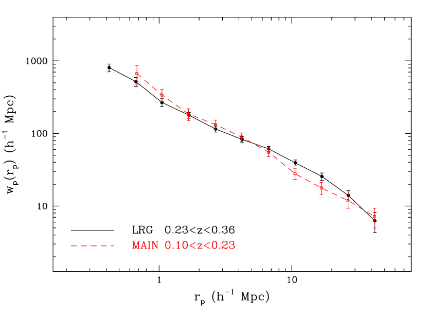
Figure 8: Projected correlation function ${w_{p}(r_{p})}$ for the $-22.6<M_{g}<-21.6$ LRG sample and the comparable one from the MAIN galaxy sample.

Now that we have demonstrated that the LRG sample extends the MAIN galaxy sample, it is interesting to compare the amplitude of the LRG clustering to that of typical $L_{*}$ galaxies. Figure 9 shows such a comparison for our largest LRG sample ($-23.2<M_{g}<-21.2$) and the $L_{*}$ MAIN galaxy sample (a volume-limited sample with $-21<M_{r}<-20$ containing $5700$ galaxies; Zehavi et al. 2004b). Note that this is in contrast to the previous comparisons (Fig. 5 and 8), where the LRG and red MAIN galaxy samples were chosen to match in luminosity and color. The quantities plotted are $[{w_{p}(r_{p})}/{w_{p}}^{fid}(r_{p})]^{1/2}$, where the fiducial ${w_{p}}^{fid}(r_{p})$ corresponds to a power-law correlation function $\xi(r)=(r/5h^{-1}{\rm\,Mpc})^{-1.8}$, and allow to infer the relative bias. For illustration purposes, we also plot this for a flat $\Lambda$CDM cosmology (with $\Omega_{m}=0.3$, $h=0.7$, $n=1$ and $\sigma_{8}=0.9$) projected correlation function computed from the nonlinear power spectrum of Smith et al. (2003) (Z. Zheng, private communication). The matter correlation function is comparable in amplitude to the $L_{*}$ MAIN correlation function, but distinct in detail. For the LRG galaxies, this scaled quantity appears roughly scale-invariant for $1-10h^{-1}{\rm\,Mpc}$, with a notable upturn on smaller scales and a downturn on large scales. When fitting a constant bias factor between the two samples, taking into account the error covariance matrices, one obtains $b_{LRG}/b_{*}=1.84\pm 0.11$ when fitting over $1h^{-1}{\rm\,Mpc}<r_{p}\lesssim 10h^{-1}{\rm\,Mpc}$. The scale dependence of the LRG inferred bias is in accord with the steeper correlation functions associated with red galaxies (e.g., Willmer, da Costa & Pellegrini 1998; Brown, Webster & Boyle 2000; Zehavi et al. 2002, 2004b). The downturn of the projected correlation function from a power-law on large separations is similar to that predicted by CDM models and to what is measured in the SDSS MAIN galaxy sample and in the 2dF survey (Hawkins et al., 2003).

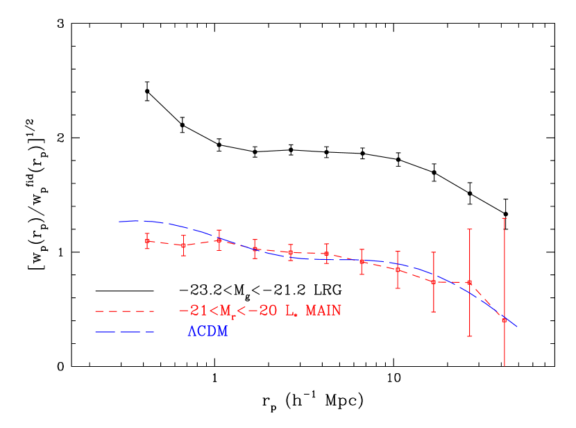
Figure 9: $[{w_{p}(r_{p})}/{w_{p}}^{fid}(r_{p})]^{1/2}$ as a function of separation $r_{p}$ for the $-23.2<M_{g}<-21.2$ LRG sample (solid symbols and line) and for the $L_{*}$ MAIN galaxy sample (open symbols and short-dashed line; Zehavi et al. 2004b), allowing to infer their relative bias. ${w_{p}}^{fid}(r_{p})$ is the projected correlation function corresponding to a fiducial power-law $\xi(r)=(r/5h^{-1}{\rm\,Mpc})^{-1.8}$. The long-dashed curve shows this relative quantity for a $\Lambda$CDM cosmology computed from the nonlinear power spectrum of Smith et al. (2003).

Real-space correlation functions have been historically well described by power laws (Totsuji & Kihara, 1969; Peebles, 1974; Gott & Turner, 1979; Davis & Peebles, 1983; Fisher et al., 1994; Jing, Mo, & Börner, 1998; Jing, Börner, & Suto, 2002; Norberg et al., 2001; Zehavi et al., 2002), although recent precision measurements provide evidence for deviations from a power-law and a means of explaining them (e.g., Berlind et al. 2003; Magliocchetti & Porciani 2003; Maller et al. 2004; Zehavi et al. 2004a; Zheng 2004). Figure 10 shows power-law fits to our projected correlation functions. The inferred $\xi(r)$ power-law fits are given in Table 3, while the ${w_{p}(r_{p})}$ measurements themselves are provided in Table 2. Inspection of the values of the correlation length, $r_{0}$, show clearly the trend with luminosity. The power-law slopes, $\gamma$, span the range 1.89 – 1.94. The $\chi^{2}/d.o.f$ values for the power-law fits are in the range $2.3-3.9$, indicating that a power-law is not a good fit. (The confidence level of a power-law fit is about 1.5% in the best case and less than 0.1% in the worst case.)

The deviations from a power-law are clearly visible in Figure 11 where we divide the clustering measurements by a representative power-law ${w_{p}(r_{p})}$ corresponding to a $\xi(r)$ with $r_{0}=10h^{-1}{\rm\,Mpc}$ and $\gamma=1.9$. Similar deviations are also seen in the complementary analysis of the LRG samples by Eisenstein et al. (2004). These deviations appear to be of a similar nature to the deviations detected in the MAIN galaxy samples (Zehavi et al., 2004a, b), which are naturally explained by contemporary models of galaxy clustering as the transition from a small-scale regime dominated by galaxy pairs in the same dark matter halo to a large-scale regime dominated by pairs of galaxies in separate halos. We delay to future work detailed halo modeling of this sort and interpretation of our measurements. There is a hint from the brightest sample of an increase at small scales ($<1h^{-1}{\rm\,Mpc}$) in the luminosity dependence of the bias, in agreement with the findings of Eisenstein et al. (2004).

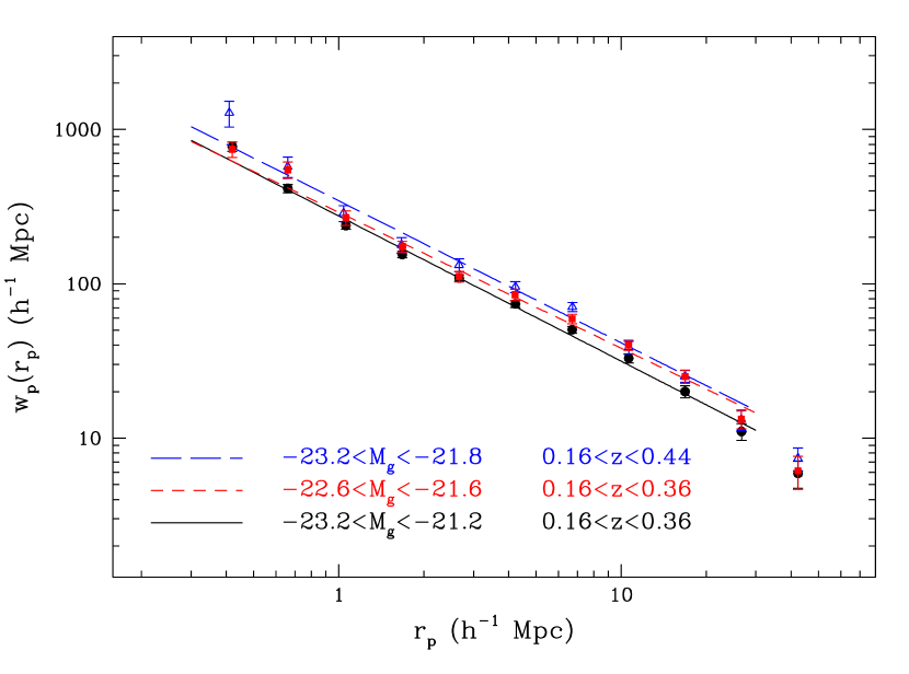
Figure 10: Projected correlation function ${w_{p}(r_{p})}$ for the three LRG samples discussed in the paper, plotted together with power-law fits fitted over the range $0.3<r_{p}<30h^{-1}{\rm\,Mpc}$.

Table 3:

$\xi(r)$ Power Law Fits
$M_{g}$ $r_{0}$ $\gamma$ $\chi^{2}/d.o.f.$ $-23.2<M_{g}<-21.2$ $9.80\pm 0.20$ $1.94\pm 0.02$ $3.9$ $-23.2<M_{g}<-21.8$ $11.21\pm 0.24$ $1.92\pm 0.03$ $3.1$ $-22.6<M_{g}<-21.6$ $10.59\pm 0.29$ $1.88\pm 0.03$ $2.3$

NOTES.—$r_{0}$ and $\gamma$ are obtained from a fit to ${w_{p}(r_{p})}$ using the full error covariance matrix. The values of $r_{0}$ are given in $h^{-1}{\rm\,Mpc}$ units.

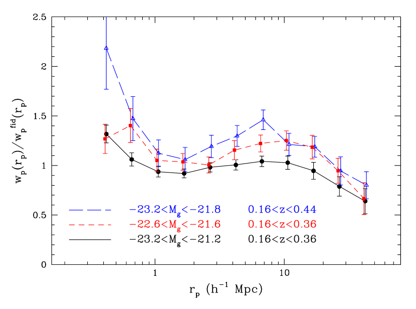
Figure 11: Projected correlation function ${w_{p}(r_{p})}$ for the LRG samples shown in Fig. 10, now all divided out by a fiducial power-law ${w_{p}(r_{p})}$ corresponding to $\xi(r)=(r/10h^{-1}{\rm\,Mpc})^{-1.9}$. The deviations from a power-law are clearly visible.

4.2 Luminosity and Redshift Dependences

Figure 12 shows the redshift dependence of the $-23.2<M_{g}<-21.8$ results. One can see small deviations of the results corresponding to the different redshift ranges. For two independent redshift shells, we estimate the best-fitting multiplicative factor, $a$, between the two ${w_{p}(r_{p})}$ measurements, taking into account the error covariance matrices. This factor would be significantly different than one if redshift evolution was present and consistent with one otherwise. The multiplicative factor between the $0.16<z<0.23$ and $0.23<z<0.36$ results is $a=0.84\pm 0.14$ and between the $0.23<z<0.36$ and $0.36<z<0.44$ measurements it is $a=1.18\pm 0.12$. For our longest redshift baseline, we find $a=1.03\pm 0.17$ between the $0.16<z<0.23$ and $0.36<z<0.44$ measurements. Converting this to a limit on $(1+z)^{n}$, we find $n=-0.2\pm 1.1$. We thus conclude that while some variations between the different redshift shells are present, these are likely to reflect large-scale structure variations, and that no consistent trend of redshift evolution is detected. We note that for the ${w_{p}(r_{p})}$ measurements for the comparable LRG and MAIN samples shown in Figure 8, $a=1.01\pm 0.10$, indicating clearly that no significant redshift evolution is present.

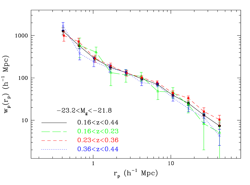
Figure 12: Redshift dependence of the ${w_{p}(r_{p})}$ clustering results for the $-23.2<M_{g}<-21.8$ sample.

We also checked the robustness of our results when calculating ${w_{p}(r_{p})}$ separately for the two large disjoint areas of the northern Galactic sky covered in the current SDSS samples. The results from these two independent regions are very similar and fully consistent, when calculated over the full redshift ranges of our samples. When looking at narrower redshift shells the differences tend to be a bit larger, reflecting the slight variations with redshift seen in Figure 12. For example, the tendency of ${w_{p}(r_{p})}$ to have a slightly lower amplitude for the $0.16<z<0.23$ shell is reproduced in the off-equatorial region, while ${w_{p}(r_{p})}$ for the equatorial region is similar to that of the full volume. This supports our conclusion that these small deviations are sample variance effects reflecting the large-scale structure fluctuations.

Figure 13 shows the projected correlation function ${w_{p}(r_{p})}$ obtained for the three LRG samples over an identical volumes ($0.16<z<0.36$). As mentioned previously, the small differences in clustering amplitude reflect the increase of clustering with luminosity. Again, we assess the significance of the increased clustering amplitude by estimating the best-fit multiplicative factor, $a$, between the measurements. Since these measurements are not fully independent (they are obtained from the same volume and thus are susceptible to similar cosmic variance effects), we cannot treat their individual error covariance matrices as independent. Instead, we estimate the value of $a$ from the mean and scatter of $a$ obtained from the individual jackknife realizations. The resulting factor between the $-23.2<M_{g}<21.8$ and $-23.2<M_{g}<21.2$ measurements is $a=1.34\pm 0.08$, more than a $4\sigma$ detection of luminosity bias. For the $-22.6<M_{g}<-21.6$ versus the $-23.2<M_{g}<21.2$ measurements, $a=1.08\pm 0.05$. It is clear that we detect a non-negligible luminosity bias among the different LRG samples.

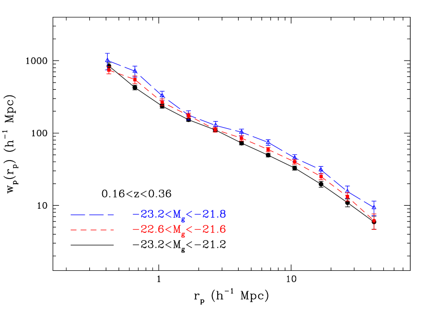
Figure 13: Luminosity dependence of ${w_{p}(r_{p})}$ obtained for the three LRG samples for $0.16<z<0.36$.

4.3 Real-Space Correlation Function

It is possible to directly invert ${w_{p}(r_{p})}$ to get $\xi(r)$ independent of the power-law assumption. This is done by recasting Equation 3 as

$$\xi(r)=-\frac{1}{\pi}\int_{r}^{\infty}dr_{p}\,{dw_{p}(r_{p})\over{dr_{p}}}({r_{p}}^{2}-r^{2})^{-1/2}.$$ (4)

(e.g., Davis & Peebles 1983). We calculate the integral analytically by linearly interpolating between the binned ${w_{p}(r_{p})}$ values, following Saunders et al. (1992). We note that this estimate is only accurate to a few percent level, due to the inaccuracy of the linear interpolation. Figure 14 presents the real-space correlation function, obtained in this fashion, for the three LRG samples. The trends with luminosity and the hints of deviations from a power-law are noticeable here as well. The $\xi(r)$ values for these samples are given as well in Table 2.

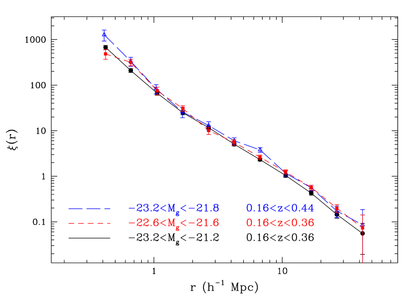
Figure 14: Real-space correlation function $\xi(r)$ for the three LRG samples.

It is common to summarize the amplitude of the correlation function as the rms variation above Poisson in the counts of galaxies in $R=8h^{-1}{\rm\,Mpc}$ comoving radius spheres. The variance $\sigma_{R}^{2}$ can be calculated as

$$\sigma_{R}^{2}=\int_{|\vec{r}_{1}|<R}d^{3}r_{1}\ \int_{|\vec{r}_{2}|<R}d^{3}r_{2}\xi(|\vec{r}_{2}-\vec{r}_{1}|)$$ (5)

where the integrals are over the interior of two spheres of radius $R$. This can be simplified to

$$\sigma_{R}^{2}=\int_{0}^{2}dy\;y^{2}\xi(yR)\left(3-{9y\over 4}+{3y^{3}\over 16}\right),$$ (6)

a useful formula that seems to have dropped out of the standard lore. Following Eisenstein (2003), we express this integral in terms of $w_{p}$ as

$$\sigma_{R}^{2}={1\over R^{3}}\int_{0}^{\infty}dr_{p}\;r_{p}w_{p}(r_{p})g(r_{p}/R)$$ (7)

where $g(x)$ is

$$\left\{\begin{array}[]{ll}{1\over 2\pi}\left[3\pi-9x+x^{3}\right]&{\rm for\ }x\leq 2,\\ {1\over 2\pi}\left[{-x^{4}+11x^{2}-28\over\sqrt{x^{2}-4}}+x^{3}-9x+6\sin^{-1}(2/x)\right]&{\rm for\ }x>2.\end{array}\right.$$

The kernel $g(x)$ is simpler than it looks: it starts positive, goes through zero at $x\approx 1.28$, and then returns to zero as $-1/\pi x^{3}$ at large $x$. It is differentiable at $x=2$.

We compute $\sigma_{8}$ by using Equation 7 and assuming that $r_{p}w_{p}(r_{p})$ is constant in each bin. This yields $\sigma_{8}=1.80\pm 0.03$ for the $-23.2<M_{g}<-21.2$ sample and $\sigma_{8}=2.06\pm 0.05$ for the $-23.2<M_{g}<-21.8$ sample, with the errors obtained from the jackknife subsamples. We stress that this is the real-space, non-linear $\sigma_{8}$, which should not be directly compared with the linear-regime $\sigma_{8}$ values that are typically quoted for CDM model normalization.

To facilitate comparison with the cross-correlations between LRGs and $L^{*}$ galaxies presented by Eisenstein et al. (2004), we also compute the following integral of the real-space correlation function:

$$\Delta={1\over V}\int_{0}^{\infty}4\pi r^{2}dr\;\xi(r)W(r),$$ (8)

where

$$W(r)={r^{2}\over a_{0}^{2}}\exp\left(-{r^{2}\over 2a_{0}^{2}}\right),$$ (9)

where $a_{0}$ is a constant scale factor. The $\Delta$ statistic isolates about one octave of scale in the real-space correlation function. For power-law correlations of the observed slopes, $\Delta(a_{0})\approx\xi(1.75a_{0})$. The $\Delta$ values are computed as a simple non-singular integral over ${w_{p}(r_{p})}$. For the $-23.2<M_{g}<-21.2$ sample, we compute $\Delta=66.5\pm 3.5$, $15.6\pm 0.7$, $4.40\pm 0.19$, and $1.31\pm 0.06$ for $a_{0}=0.5h^{-1}{\rm\,Mpc}$, $1h^{-1}{\rm\,Mpc}$, $2h^{-1}{\rm\,Mpc}$, and $4h^{-1}{\rm\,Mpc}$ proper distance at $z=0.3$. These scales are chosen to match those in Eisenstein et al. (2004). For the $-23.2<M_{g}<-21.8$ sample, the $\Delta$ values are $91.8\pm 9.6$, $18.1\pm 1.8$, $5.54\pm 0.43$, and $1.73\pm 0.12$, respectively.

5 Conclusions

We have presented a statistical analysis of the intermediate-scale ($0.3$ to $40h^{-1}{\rm\,Mpc}$) correlations of $35,000$ luminous red galaxies from the SDSS, using three nearly volume-limited subsamples. The size of the sample permits measurements of superb precision for these rare galaxies. We find clear deviations from power-law models in the projected correlation functions. Relative to a power-law, there are excesses of clustering on sub-Mpc scales and at $5-10$ Mpc scales. These match qualitatively the deviations found in the SDSS MAIN sample galaxies and predicted by halo modeling (Zehavi et al., 2004a, b).

The SDSS LRG sample reproduces the clustering results obtained with the SDSS MAIN galaxy sample when matched appropriately in magnitude and color and thus provides an extension of the galaxy clustering analyses to higher redshifts, and a better signal-to-noise measurement of high luminosity galaxies. We find no evidence for redshift evolution of the correlation functions (for a fixed passively evolving magnitude range) out to $z=0.4$. However, the errors are such that dependences even as strong as $(1+z)^{\pm 2}$ cannot be excluded at more than $2\sigma$.

All of the LRG samples are highly clustered, with correlation lengths around $10h^{-1}{\rm\,Mpc}$ comoving, roughly twice that of $L_{*}$ galaxies (e.g., Norberg et al. 2001; Zehavi et al. 2002, 2004b). For the $-23.2<M_{g}<-21.2$ LRGs, the inferred bias relative to that of $L_{*}$ galaxies is $1.84\pm 0.11$ on scales of $1-10h^{-1}{\rm\,Mpc}$. The bias is roughly scale invariant on these scales and shows stronger clustering on smaller scales.

We find that more luminous LRGs are yet more clustered; however, none of our samples reach the correlation levels of rich clusters (Bahcall & Soneira, 1983; Nichol et al., 1992; Peacock & West, 1992; Croft et al., 1997; Abadi et al., 1998; Lee & Park, 1999; Collins et al., 2000; Gonzalez, Zaritsky & Wechsler, 2002; Bahcall et al., 2003). Note that all the latter estimate the cluster redshift-space correlation function, and thus should be compared to our $s_{0}$ values inferred from Table 2 and not the $r_{0}$ values quoted in Table 3. The LRG clustering strengths and mean separations $d$ are comparable to those of the poorest clusters mentioned in these works. Our measurements are roughly consistent with the Bahcall et al. (2003) trend of increasing correlation length with mean separation, $s_{0}=2.6\sqrt{d}$ (see also their Fig. 2). The LRG clustering strength we find is comparable as well to that of rich groups, which again have similar mean separations (Padilla et al., 2004; Yang et al., 2004).

The SDSS LRG sample offers an enormous data set for the study of rare but important massive early-type galaxies. The interplay of number density, clustering amplitude, correlation function shapes, redshift distortions, and higher-order correlations will provide a rich data set for the modeling of the relationship of these galaxies to their host halos and thereby to the evolution of the extreme end of the galaxy mass function.

A Modeling of Selection Functions

A.1 Redshift Distribution

To perform a 3-dimensional correlation analysis, one must have a model for the expected number of galaxies (in the absence of clustering) as a function of redshift at every point on the sky. Often this is done by computing a luminosity function and then integrating to a given depth. In the case of the LRG sample, this is hard to implement reliably because the luminosity function is so steep that minor variations in the $k$ and $e$ corrections are important and because the color selection does not select the identical region of rest-frame color-luminosity space at all redshifts.

Instead, we construct an approximate model of the redshift distribution based on models of the selection and then low-pass fit this model to the observed redshift distribution. This removes power on very large radial separation scales (below $k=0.04h{\rm\,Mpc}^{-1}$), but provides an excellent model for smaller scales.

In detail, we predict the $g-r$ and $r-i$ colors of early-type galaxies as a function of redshift by convolving the observed average LRG spectrum (Eisenstein et al., 2003) with the SDSS system response. We then tweak that color-redshift relation onto the observed photometry with low-pass filtering. The spectral breaks of early-type galaxies create subtle features in the color-redshift relation that are currently difficult to resolve in the empirical photometry. At each redshift, we create a Monte Carlo set of colors by adding Gaussian noise to the mean color. We then find how luminous a galaxy would have to be to pass the LRG selection cut (this is a highly sensitive function of color) and integrate a hypothesized passively-evolved luminosity function, following Blanton et al. (2003b), to find the number of galaxies. Summing over the Monte Carlo points and multiplying by the cosmological volume gives the predicted real density of galaxies per redshift bin for a passively-evolving model population. This distribution is forced onto the observed redshift distribution using a boxcar smoothing length of 0.07 in redshift. Our resulting model is shown as the solid line in Figures 1, 2, and 3. This more complex procedure is needed as, note, for example, the bump at $z=0.34$ that is caused by the G band absorption feature moving from the $g$ to $r$ filter. A simple boxcar smoothing of the redshift histogram does not preserve the height of this feature, but predicting the height from the average LRG spectrum produces an excellent match.

A.2 Angular Selection Function

Selected galaxies can fail to receive spectra for three major reasons: 1) they might fall within the fiber collision radius $55^{\prime\prime}$ of another target and not get assigned a fiber, 2) the plate to which they were assigned might not have been observed yet, and 3) they might have fallen outside of the boundary of any plate. With the adaptive tiling of the survey, it is very rare for an isolated object inside a plate boundary to fail to be placed on the plate.

We weight the LRGs to account for fiber collisions by using a friends-of-friends grouping algorithm with a $55^{\prime\prime}$ linking length (provided within the lss_sample14 package) run on all of the galaxy and quasar targets. Within each collision group, we find the number of objects that did get assigned to a plate and divide by the total number. The inverse of this is the weighting assigned to the LRGs that did get assigned to plates. Note that to the extent that the selection of targets within the collision group was strictly random, this approach is the correct procedure for two-point clustering on separations larger than $55^{\prime\prime}$, even if the colliding objects are at very different redshifts. Imagine that there are two objects in close proximity and we wish to study the correlations with a third distant object (e.g., to count the pairs). In a perfect survey, one would have two pairs, each with a different redshift separation. In one version of the SDSS, one of the pairs would be counted, but with double weight; in another version, the other pair would be counted with double weight. The ensemble average over many such examples is unbiased with respect to the result of the perfect survey. Only the pair corresponding to the two close objects is being mistreated (as it will never exist in this example), but that pair only matters for very small separation structure. In truth, the priorities of all targets are not quite equal, such that LRGs will always lose to quasar candidates, but the priority is equal to the dominant MAIN targets. The key angular separation of $55^{\prime\prime}$ corresponds to $0.22h^{-1}{\rm\,Mpc}$ at $z=0.3$, and we thus restrict our measurements to separations larger than that.

The lss_sample14 package provides the angular geometry of the spectroscopic survey expressed in terms of spherical polygons. The geometry is complicated: the spectroscopic plates are circular and overlap, while the imaging is in long strips on the sky and there are some overlap regions of certain plates that may not have been yet observed. The resulting spherical polygons track all these effects and characterize the geometry in terms of “sectors”, each being a unique region of overlapping spectroscopic plates. In each sector, we count the number of possible targets (LRG, MAIN, and quasar), excluding those missed because of fiber collisions, and the number of these that did get a spectrum. We weight the galaxies by the ratio of these numbers. Typically, this ratio is very close to unity (mean of $1.007$). It is large only in instances of regions covered by two plates where one of the plates has not yet been observed. To exclude these extreme cases, we cut our sample at a ratio of $1.67$, which eliminates $550$ LRG spectra.

We also mask from the sample any regions that are close to bright (heavily saturated) stars. At present, we have not included any other masking. Notably, we are not explicitly excluding regions because of high reddening or poor image quality; however, such regions are typically not targeted for spectroscopy and would already have been excluded from the above geometry. We are not masking out small-scale imaging defects such as saturation trails or satellite tracks, nor avoiding the region around bright galaxies. These involve less than $1\%$ of the survey area and have negligible effects on the strong clustering signal shown by LRGs. We treat the boundaries of the spectroscopic plates as simple boundaries of the survey. In other words, we neglect any correlation between these real-world boundaries and the LRG distribution. Since the LRGs are a subdominant population with mild angular clustering, it is very unlikely that there is any important cross-talk between the LRG distribution and regions missed because of the adaptive tiling.

A.3 Color Calibration Issues

A persistent worry with clustering of SDSS LRGs is the high sensitivity of the selection to errors in the photometric calibration (Eisenstein et al., 2001). Errors of 1% in $r-i$ create 8% fluctuations in the number density of the $-23.2<M_{g}<-21.2$ sample, although the other samples are more robust because their minimum luminosities are not close to the selection boundary and the selection variations with absolute magnitude are three times less than those with $r-i$ color. Obviously, errors in the photometric zeropoints will be correlated on the sky, leaving long stripes of false density fluctuations on the sky.

However, the SDSS has demonstrated 2% rms calibrations (Abazajian et al., 2004), which would produce only 0.025 effects in the correlation function. Moreover, we find that this is an overestimate because the calibration errors are for the most part only correlated along the SDSS stripes, not between them. As the calibrations are applied by secondary patches that are only about 0.6 degrees wide (Stoughton et al., 2002), the calibration errors are suppressed on larger angular scales. We see no indication of any significant effect on the scales in this paper from calibration effects.

References

- Abadi et al. (1998) Abadi, M., Lambas, D., & Muriel, H. 1998, ApJ, 507, 526
- Abazajian et al. (2004) Abazajian, K., et al. 2004, AJ, 128, 502
- Bahcall et al. (2003) Bahcall, N.A., Dong, F., Hao, L., Bode, P., Annis, J., Gunn, J.E., Schneider, D.P., 2003, ApJ, 599, 814
- Bahcall & Soneira (1983) Bahcall, N. A., & Soneira, R. M. 1983, ApJ, 270, 20
- Bardeen et al. (1986) Bardeen, J.M., Bond, J.R., Kaiser, N., & Szalay, A.S., 1986, ApJ, 304, 15
- Benoist et al. (1996) Benoist, C., Maurogordato, S., da Costa, L. N., Cappi, A., & Schaeffer, R. 1996, ApJ, 472, 452
- Benson et al. (2000) Benson, A. J., Cole, S., Frenk, C. S., Baugh, C. M., & Lacey, C. G. 2000, MNRAS, 311, 793
- Berlind & Weinberg (2002) Berlind, A. A., & Weinberg, D. H. 2002, ApJ, 575, 587
- Berlind et al. (2003) Berlind, A. A., Weinberg, D. H., Benson, A. J., Baugh, C. M., Cole, S., et al. 2003, ApJ, 593, 1
- Blanton et al. (2003a) Blanton, M.R., Lupton, R.H., Maley, F.M., Young, N., Zehavi, I., Loveday, J., 2003a, AJ, 125, 2276
- Blanton et al. (2003b) Blanton, M. R., et al. 2003b, ApJ, 592, 819
- Brown, Webster & Boyle (2000) Brown, M. J. I., Webster, R. L., & Boyle, B. J. 2000, MNRAS, 317, 782
- Budavari et al. (2003) Budavari, T., et al. 2003, ApJ, 595, 59
- Carlberg et al. (2001) Carlberg, R. G., Yee, H. K. C., Morris, S. L., Lin, H., Hall, P. B., Patton, D. R., Sawicki, M., & Shepherd, C. W. 2001, ApJ, 563, 736
- Collins et al. (2000) Collins, C., et al. 2000, MNRAS, 319, 939
- Connolly et al. (2002) Connolly, A., et al. 2002, ApJ, 579, 42
- Croft et al. (1997) Croft, R. A. C., et al. 1997, MNRAS, 291, 305
- Davis & Geller (1976) Davis, M., & Geller, M. J. 1976, ApJ, 208, 13
- Davis & Peebles (1983) Davis, M., & Peebles, P. J. E. 1983, ApJ, 267, 465
- Dressler (1980) Dressler, A. 1980, ApJ, 236, 351
- Eisenstein et al. (2001) Eisenstein, D.J., et al. 2001, AJ, 122, 2267
- Eisenstein (2003) Eisenstein, D.J., 2003, ApJ, 586, 718
- Eisenstein et al. (2003) Eisenstein, D.J., et al. 2003, ApJ, 585, 694
- Eisenstein et al. (2004) Eisenstein, D.J., Blanton, M. R., Zehavi, I., Bahcall, N. A., Brinkmann, J., Loveday, J., & Meiksin, A. 2004, ApJ, in press
- Fisher et al. (1994) Fisher, K. B., Davis, M., Strauss, M. A., Yahil, A., & Huchra, J. P. 1994, MNRAS, 266, 50
- Fukugita et al. (1996) Fukugita, M., Ichikawa, T., Gunn, J. E., Doi, M., Shimasaku, K., & Schneider, D. P. 1996, AJ, 111, 1748
- Gonzalez, Zaritsky & Wechsler (2002) Gonzalez, A. H., Zaritsky, D., & Wechsler, R. H. 2002, ApJ, 571, 129
- Gott & Turner (1979) Gott, J. R., & Turner, E. L. 1979, ApJ, 232, L79
- Gunn et al. (1998) Gunn, J.E., et al., 1998, AJ, 116, 3040
- Guzzo et al. (1997) Guzzo, L., Strauss, M. A., Fisher, K. B., Giovanelli, R., & Haynes, M. P. 1997, ApJ, 489, 37
- Hamilton (1988) Hamilton, A. J. S. 1988, ApJ, 331, L59
- Hamilton (1993) Hamilton, A. J. S. 1993, ApJ, 417, 19
- Hawkins et al. (2003) Hawkins, E., et al. 2003, MNRAS, 346, 78
- Hoessel et al. (1980) Hoessel, J. G., Gunn, J. E., Thuan, T. X., 1980, ApJ, 241, 486
- Hogg et al. (2001) Hogg, D. W., Finkbeiner, D. P., Schlegel, D. J., & Gunn, J. E. 2001, AJ, 122, 2129
- Hogg et al. (2003) Hogg, D. W., et al. 2003, ApJ, 585, L5
- Hubble (1936) Hubble, E.P. 1936, The Realm of the Nebulae (Oxford University Press: Oxford), 79
- Jing, Börner, & Suto (2002) Jing, Y. P., Börner, G., & Suto, Y. 2002, ApJ, 564, 15
- Jing, Mo, & Börner (1998) Jing, Y. P., Mo, H. J., & Börner, G. 1998, ApJ, 494, 1
- Kauffmann, Nusser, & Steinmetz (1997) Kauffmann, G., Nusser, A., & Steinmetz, M. 1997, MNRAS, 286, 795
- Kauffman et al. (1999) Kauffmann, G., Colberg, J. M., Diaferio, A., & White, S. D. M. 1999, MNRAS, 303, 188
- Kaiser (1984) Kaiser, N. 1984, ApJ, 294, L9
- Kravtsov et al. (2004) Kravtsov, A. V., Berlind, A. A., Wechsler, R. H., Klypin, A. A., Gottloeber, S., Allgood, B., & Primack, J. R. 2004, ApJ, 609, 35
- Landy & Szalay (1993) Landy, S. D., & Szalay, A. S. 1993, ApJ, 412, 64
- Lee & Park (1999) Lee, S., & Park, C. 1999, JKAS, 31, 1
- Loveday et al. (1995) Loveday, J., Maddox, S. J., Efstathiou, G., & Peterson, B. A. 1995, ApJ, 442, 457
- Lupton et al. (2001) Lupton, R., Gunn, J.E., Ivezić, Z., Knapp, G.R., Kent, S., & Yasuda, N. 2001, in ASP Conf. Ser. 238, Astronomical Data Analysis Software and Systems X, ed. F. R. Harnden, Jr., F. A. Primini, and H. E. Payne (San Francisco: Astr. Spc. Pac.); astro-ph/0101420
- Ma & Fry (2000) Ma, C., & Fry, J. N. 2000, ApJ, 543, 503
- Madgwick et al. (2003) Madgwick, D. S. et al. 2003, MNRAS, 344, 847
- Magliocchetti & Porciani (2003) Magliocchetti, M., & Porciani, C., 2003, MNRAS, 344, 847
- Maller et al. (2004) Maller, A. H., McIntosh, D. H., Katz, N., & Weinberg, M. D. 2004, ApJ, in press (astro-ph/0304005)
- Mo & White (1996) Mo, H. J., & White, S. D. M. 1996, MNRAS, 282, 1096
- Nichol et al. (1992) Nichol, R. C., Collins, C. A., Guzzo, L., & Lumsden, S. L. 1992, MNRAS, 255, 21
- Norberg et al. (2001) Norberg, P., et al. 2001, MNRAS, 328, 64
- Norberg et al. (2002) Norberg, P., et al. 2002, MNRAS, 332, 827
- Padilla et al. (2004) Padilla, N. D., et al. 2004, MNRAS, 352, 211
- Park et al. (1994) Park, C., Vogeley, M. S., Geller, M. J., & Huchra, J. P. 1994, ApJ, 431, 569
- Peacock & Smith (2000) Peacock, J. A., & Smith, R. E. 2000, MNRAS, 318, 1144
- Peacock & West (1992) Peacock, J. A., & West, M. J. 1992, MNRAS, 259, 494
- Peebles (1974) Peebles, P. J. E. 1974, A& A 32, 197
- Pier et al. (2003) Pier, J. R., Munn, J. A., Hindsley, R. B., Hennessy, G. S., Kent, S. M., Lupton, R. H., & Ivezic, Z. 2003, AJ, 125, 1559
- Postman & Geller (1984) Postman, M., & Geller, M. J. 1984, ApJ, 281, 95
- Postman & Lauer (1995) Postman, M. & Lauer, T.R., 1995, ApJ, 440, 28
- Sandage (1972) Sandage, A., 1972, ApJ, 178, 1
- Saunders et al. (1992) Saunders, W., Rowan-Robinson, M., & Lawrence, A. 1992, MNRAS, 258, 134
- Schneider et al. (1983) Schneider, D.P., Gunn, J.E., Hoessel, J.G., 1983, ApJ, 264, 337
- Scoccimarro et al. (2001) Scoccimarro, R., Sheth, R. K., Hui, L., & Jain, B. 2001, ApJ, 546, 20
- Seljak (2000) Seljak, U. 2000, MNRAS, 318, 203
- Sheth, Mo, & Tormen (2001) Sheth, R. K., Mo, H. J., & Tormen, G. 2001, MNRAS, 323, 1
- Smith et al. (2002) Smith, J. A., Tucker, D. L. et al. 2002, AJ, 123, 2121
- Smith et al. (2003) Smith, R. E., et al. 2003, MNRAS, 341, 1311
- Stoughton et al. (2002) Stoughton, C. et al. 2002, AJ, 123, 485
- Strauss et al. (2002) Strauss, M.A., et al. 2002, AJ, 124, 1810
- Tegmark et al. (2004) Tegmark, M., et al. 2004, ApJ, 606, 702
- Totsuji & Kihara (1969) Totsuji, H., & Kihara, T. 1969, PASJ, 21, 221
- White, Tully, & Davis (1988) White, S. D. M., Tully, R. B., & Davis, M. 1988, ApJ, 333, L45
- Willmer, da Costa & Pellegrini (1998) Willmer, C. N. A., da Costa, L. N., & Pellegrini, P. S. 1998, AJ, 115, 869
- Yang et al. (2004) Yang, X., Mo, H.J., van den Bosch, F.C., Jing, Y.P., 2004, MNRAS, submitted (astro-ph/0406593)
- York et al. (2000) York, D.G., et al. 2000, AJ, 120, 1579
- Zehavi et al. (2002) Zehavi, I., Blanton, M.R., Frieman, J.A., Weinberg, D.H., Mo, H.J., et al. 2002, ApJ, 571, 172
- Zehavi et al. (2004a) Zehavi, I., Weinberg, D.H., Zheng, Z., Berlind, A.A., Frieman, J.A., et al. 2004a, ApJ, 608, 16
- Zehavi et al. (2004b) Zehavi, I., et al. 2004b, ApJ, submitted (astro-ph/0408569)
- Zheng (2004) Zheng, Z. 2004, ApJ, 610, 61
- Zwicky et al. (1968) Zwicky, F., Herzog, E., Wild, P., Karpowicz, M., & Kowal, C., 1961-1968, Catalog of Galaxies and of Clusters of Galaxies, Vols. 1-6, (Pasadena: California Institute of Technology)