The Small-scale Clustering of Luminous Red Galaxies via Cross-Correlation Techniques

Abstract

We present the small-scale ($0.2h^{-1}$ to $7h^{-1}$ Mpc) cross-correlations between 32,000 luminous early-type galaxies and a reference sample of 16 million normal galaxies from the Sloan Digital Sky Survey. Our method allows us to construct the spherically averaged, real-space cross-correlation function between the spectroscopic LRG sample and galaxies from the SDSS imaging. We report the cross-correlation as a function of scale, luminosity, and redshift. We find very strong luminosity dependences in the clustering amplitudes, up to a factor of 4 over a factor of 4 in luminosity, and measure this dependence with high signal-to-noise ratio. The luminosity dependence of bias is found to depend on scale, with more variation on smaller scales. The clustering as a function of scale is not a power law, but instead has a dip at $1h^{-1}{\rm\,Mpc}$ and an excess on small scales. The fraction of red galaxies within the $L^{*}$ sample surrounding LRGs is a strong function of scale, as expected. However, the fraction of red galaxies evolves in redshift similarly on small and large scales, suggesting that cluster and field populations are changing in the same manner. The results highlight the advantage on small scales of using cross-correlation methods as a means of avoiding shot noise in samples of rare galaxies.

Draft in progress,

1 Introduction

Galaxy clustering allows us to study the relation of galaxies to dark matter through the biased clustering of dark matter halos and to probe the possibility of environment-dependent processes in the evolution of galaxies. With today’s large galaxy surveys, we can measure this clustering at very high signal-to-noise ratio, investigating the detailed trends of clustering with luminosity, color, morphology, and redshift (Hubble, 1936; Zwicky et al., 1968; Davis & Geller, 1976; Dressler, 1980; Postman & Geller, 1984; Hamilton, 1988; White, Tully, & Davis, 1988; Park et al., 1994; Loveday et al., 1995; Guzzo et al., 1997; Benoist et al., 1998; Willmer, da Costa & Pellegrini, 1998; Brown, Webster & Boyle, 2000; Carlberg et al., 2001; Norberg et al., 2001; Zehavi et al., 2002; Norberg et al., 2002; Budavari et al., 2003; Madgwick et al., 2003; Hogg et al., 2003a; Zehavi et al., 2004b).

Massive galaxies are particularly interesting to study via clustering analyses because they tend to reside in massive dark matter halos (Sandage, 1972; Hoessel et al., 1980; Schneider et al., 1983; Postman & Lauer, 1995). These halos themselves have strong trends of clustering amplitude versus mass (Kaiser, 1984; Bardeen et al., 1986; Mo & White, 1996; Sheth, Mo, & Tormen, 2001), implying that one can find significant variations in clustering whenever the mean halo mass of the subsample galaxies is changed. Moreover, because massive galaxies are roughly passively evolving at low redshifts (McCarthy et al., 2001; Fontana et al., 2004; Glazebrook et al., 2004, but see Drory et al. 2004), we should be able to interpret the redshift evolution of clustering. A fixed set of galaxies cannot be in high-mass halos at one redshift and low-mass halos at the next, whereas a set defined by a more transitory identifier, such as strong star formation, need not be found in a consistent location from one time to another.

Here, we use a sample of very luminous early-type galaxies from the Sloan Digital Sky Survey (SDSS; York et al. 2000) to measure the small-scale clustering ($0.2h^{-1}$ to $7h^{-1}{\rm\,Mpc}$) of the most massive galaxies. We do this by use of angular cross-correlations between 32,000 luminous red galaxies (LRG) with spectroscopic redshifts and 16 million fainter galaxies from the SDSS imaging survey. The method of Eisenstein (2003) constructs spherically symmetric measurements of the real-space spatial cross-correlation function in a flexible manner that supports investigations of many different potential trends. We have previously applied the method to the study of low-redshift galaxies in the SDSS (Hogg et al., 2003a; Blanton et al., 2003c). We focus here on the luminosity, scale, and color dependence of the clustering of $\sim\!L^{*}$ galaxies surrounding the LRGs.

The application to LRGs shows the considerable advantages of the cross-correlation of spectroscopic and imaging data sets for the study of small-scale clustering of rare populations. By avoiding auto-correlation, we remove a large amount of shot noise from the computation at only a minor cost in signal. Moreover the flexibility of the method recommends it to topics involving trends in multi-dimensional parameter spaces. We expect that the method will find applications in higher redshift work as well.

As tracers of high-density regions, massive early-type galaxies also offer a way to study the environmental dependences of nearby fainter galaxies via cross-correlation techniques. We do this by using the colors of the galaxies in the imaging sample to measure the fraction of red galaxies as a function of redshift and distance from the LRG. Of course, there is a strong gradient in red fraction as a function of distance (Hubble & Humason, 1931; Abell, 1965; Oemler, 1974; Melnick & Sargent, 1977; Dressler, 1980; Postman & Geller, 1984). The time evolution of the red fraction as a function of environment is one of the more studied quantities in extragalactic astrophysics, in clusters as the Butcher-Oemler effect (e.g., Butcher & Oemler, 1978, 1984; Dressler & Gunn, 1983; Lavery & Henry, 1986) and in the field as the faint blue galaxy problem (e.g., Broadhurst et al., 1988; Tyson, 1988; Jones et al., 1991; Lilly et al., 1991; Metcalfe et al., 1991) and the evolution of the star formation density (e.g., Lilly et al., 1996; Madau et al., 1996). While all agree that these reddening trends are a window into galaxy evolution, the questions of whether this evolution is environmentally dependent and what processes underlie it remain controversial (e.g., Hashimoto et al., 1998; Balogh et al., 1999; Margoniner et al., 2001; de Propris et al., 2004).

The outline of this paper is as follows. §2 reviews the methodology employed, with more detail provided in Appendices A and B. §3 describes the samples of spectroscopic and imaging galaxies we use. We present the results in §4 and conclude in §5. We use a $\Omega_{m}=0.3$ flat cosmology throughout and quote magnitudes with $h=1$. All magnitudes have been corrected for reddening using the Schlegel et al. (1998) map.

2 Cross-correlation methodology

We will use the angular cross-correlation method described in Eisenstein (2003). In this method, one cross-correlates a sample of known redshift with a sample of unknown redshift. The first sample will be spectroscopic galaxies from the SDSS; the second sample will be galaxies from the SDSS imaging catalogs. To the extent that gravitational lensing can be neglected (justified in Appendix B), the only physical correlations are at similar redshift, and so one can use the known redshift of one object of each pair to translate angles into transverse distances and fluxes into luminosities (Davis et al., 1978; Yee & Green, 1987; Phillipps & Shanks, 1987; Lilje & Efstathiou, 1988; Ferguson & Sandage, 1991; Vader & Sandage, 1991; Saunders et al., 1992; Lorrimer et al., 1994; Loveday, 1997). For example, we will use the known redshift to select a fixed luminosity range for our imaging sample.

It is well-known that the assumption of isotropic clustering permits one to deproject angular correlations into true spatial correlations (von Zeipel, 1908; Fall & Tremaine, 1977; Davis et al., 1978; Phillipps, 1985; Saunders et al., 1992; Baugh & Efstathiou, 1993; Loveday, 1997; Dodelson & Gaztañaga, 2000; Eisenstein & Zaldarriaga, 2001). The method of Eisenstein (2003) performs this deprojection but notes that the noisy derivative that usually enters can be avoided by integrating the real-space spatial correlation function (denoted ${\xi_{\rm is}}$) on spherical windows:

$$\Delta={1\over V}\int_{0}^{\infty}4\pi r^{2}dr\;{\xi_{\rm is}}(r)W(r)$$ (1)

where $W$ is our smoothing window and $V=\int_{0}^{\infty}4\pi r^{2}dr\;W(r)$. The resulting quantity $\Delta$ is physically useful: it is the average overdensity of objects from the imaging catalog in the neighborhood (as defined by $W$) of a spectroscopic object. $\Delta$ of course depends on $W(r)$, which in turn will have a characteristic scale $a$. Hence, $\Delta$ is a function of $a$, although we suppress the label.

Eisenstein (2003) demonstrates that the quantity $\Delta$ can be estimated simply by a pairwise summation over the two catalogs with a weighting function $G(R)$, defined by

$$G(R) = {1\over R}{dF\over dR}$$ (2)

$$F(R) = {2\over\pi}\int_{0}^{R}dr\;{r^{2}W(r)\over\sqrt{R^{2}-r^{2}}}$$ (3)

Explicitly, we have

$$\Delta={1\over N_{sp}}\sum_{j\in\{sp\}}{1\over\phi_{0}(z_{j})V}\sum_{k\in\{im\}}G(R_{jk})$$ (4)

where the sums are over the spectroscopic and imaging catalogs, respectively. $N_{sp}$ is the number of spectroscopic objects, $R_{jk}$ is the transverse distance between the two objects (using the angle and the angular diameter distance to the given redshift), and $\phi_{0}(z_{j})$ is the space density of the objects from the imaging catalog at the given redshift. This double summation can then be conveniently split, to define a value of $\Delta$ for each spectroscopic object:

$$\Delta_{j}={1\over\phi_{0}(z_{j})V}\sum_{k\in\{im\}}G(R_{jk}).$$ (5)

We can tabulate these $\Delta_{j}$ for each spectroscopic object and then take the average for any subset we wish. This allows us to find the run of overdensity versus redshift and luminosity and to perform jackknife resamplings with essentially no overhead. It also makes clear that there is no need to bin the spectroscopic galaxies in redshift before computing. Appendix A describes how we account for masks and efficiently handle the summation over large-separation pairs.

Note that the space density of the imaging catalog as a function of redshift, $\phi_{0}(z)$, is not necessarily known. By choosing a sliding flux limit in the imaging catalog as a function of the spectroscopic object’s redshift, we minimize the change in $\phi_{0}(z)$ while also keeping the reference sample as constant as possible, so that clustering amplitudes can be most easily related to clustering bias. It is important to note that even if $\phi_{0}(z)$ is unknown, the relative values of $\Delta$ between different scales and different luminosities of the spectroscopic galaxies are still accurately known. In other words, we can study differential effects at a single redshift and even the redshift evolution of those differential effects. Only the absolute clustering amplitudes as a function of redshift depend on the modeling of $\phi_{0}(z)$.

We will use windows of the form

$$W(r)={r^{2}\over a^{2}}\exp\left(-{r^{2}\over 2a^{2}}\right)$$ (6)

where $a$ is a scale length. This choice allows us to focus on about one factor of two of scale in the cross-correlation ${\xi_{\rm is}}(r)$. The apodization at small scale improves on a pure Gaussian window in that it downweights very small-angle pairs where object deblending might be a concern.

For this choice, the required $F$ and $G$ functions are

$$F(R) = 4a^{2}se^{-s}\left[2sI_{0}(s)-(1+2s)I_{1}(s)\right]$$ (7)

$$G(R) = se^{-s}\left[(6-8s)I_{0}(s)+(-2+8s)I_{1}(s)\right]$$ (8)

where $s=R^{2}/4a^{2}$ and $I_{0}$ and $I_{1}$ are modified Bessel functions of the first kind. For coding, it is useful to note that

$$G(R)\approx{-1\over\sqrt{2\pi s^{3}}}\left[{3\over 4}+{45\over 32s}+{1575\over 512s^{2}}+O(s^{-3})\right]$$ (9)

for large $s$. We see that $G\approx 3R^{2}/2a^{2}$ at small $R$, so small separation pairs are indeed downweighted. For this window, $V=3a^{3}(2\pi)^{3/2}$.

For a power-law ${\xi_{\rm is}}(r)\propto r^{-1-\alpha}$, the resulting connection between $\Delta$ and ${\xi_{\rm is}}$ is

$$\Delta={2\over 3}\sqrt{2\over\pi}\sqrt{2}^{-\alpha}\Gamma\left(2-{\alpha\over 2}\right){\xi_{\rm is}}(a).$$ (10)

For $\alpha=0.8$, this means that $\Delta=0.36{\xi_{\rm is}}(a)\approx{\xi_{\rm is}}(1.76a)$. For $\alpha=1.0$, $\Delta={\xi_{\rm is}}(a)/3\approx{\xi_{\rm is}}(1.73a)$. In other words, we are roughly measuring the correlation function on the scale $1.75a$. This shift is not surprising in that $W(r)$ has most of its weight at $r>a$.

We will compute the mean environment for many different luminosity bins, redshift bins, scale lengths, and two imaging galaxy samples. The errors on each data point are estimated by jackknife resampling. We use 50 spatially coherent subsamples of the data for the resamplings. We have investigated the covariances between different measurements. Of course, different scale lengths and imaging samples for the same primary LRG bins are highly covariant, typically 50-70% correlated between scales separated by a factor of two. However, we find that different luminosity and redshift bins are generally close to independent. This is expected: there are not many LRGs in a given large non-linear structure.

We will use proper (i.e. non-comoving) distances throughout this paper. The reason is that with this choice the computed quantity $\phi_{0}\Delta$ is predicted to be redshift independent for the stable clustering ansatz (Peebles, 1980). This is easy to see because $\phi_{0}V\Delta$ is the number of imaging galaxies surrounding the spectroscopic galaxy, and stable clustering predicts that these structures are time independent. On much larger scales, linear perturbation theory (e.g. Peebles, 1980) predicts $\phi_{0}\Delta\propto(1+z)^{-n}D^{2}$ for a fixed proper scale, where $D(z)$ is the growth function (perhaps generalized to include the evolution of bias) and $n$ is the power-spectrum spectral index $P\propto k^{n}$; for concordance cold dark matter cosmologies, this prediction is also close to constant if the bias is time-independent. Aside from the aesthetics of a constant baseline hypothesis, the choice of non-comoving distances also makes it simple to average over redshifts if the spectroscopic sample is imperfectly volume-limited. In practice, we average $\phi(z)\Delta$ rather than $\Delta$, as the former is empirically close to constant in redshift.

Appendix B argues that the effects of weak lensing are only of order 1% for the results in this paper. This is slightly below our best 1–$\sigma$ errors. We therefore neglect gravitational lensing. False correlations imprinted by photometric calibration errors common to the two samples are shown Appendix A to be negligibly small for this application.

3 SDSS samples

3.1 Description of the SDSS

The SDSS (York et al., 2000; Stoughton et al., 2002; Abazajian et al., 2003, 2004) is imaging $10^{4}$ square degrees away from the Galactic Plane in 5 passbands, $u$, $g$, $r$, $i$, and $z$ (Fukugita et al., 1996; Gunn et al., 1998). Image processing (Lupton et al., 2001; Stoughton et al., 2002; Pier et al., 2003) and calibration (Hogg et al., 2001; Smith, Tucker et al., 2002) allow one to select galaxies, quasars, and stars for follow-up spectroscopy with twin fiber-fed double-spectrographs. The spectra cover 3800Å to 9200Å with a resolution of 1800. Targets are assigned to plug plates with a tiling algorithm that ensures nearly complete samples (Blanton et al., 2003a).

Galaxy spectroscopic target selection proceeds by two algorithms. The primary sample (Strauss et al., 2002), referred to here as the MAIN sample, targets galaxies brighter than $r<17.77$. The surface density of such galaxies is about 90 per square degree. The LRG algorithm (Eisenstein et al., 2001) selects $\sim\!12$ additional galaxies per square degree, using color-magnitude cuts in $g$, $r$, and $i$ to select galaxies to $r<19.5$ that are likely to be luminous early-types at redshifts up to $\sim\!0.5$. The selection is extremely efficient, and the redshift success rate is very high. A few galaxies (3 per square degree at $z>0.15$) matching the rest-frame color and luminosity properties of the LRGs are extracted from the MAIN sample; we refer to this combined set as the LRG sample. In detail, there are two sections of the LRG algorithm, known as Cut I and Cut II and described in Eisenstein et al. (2001).

We begin from a spectroscopic sample covering 3,836 square degrees. The exact survey geometry is expressed in terms of spherical polygons and is known as lss_sample14. This set contains 55,000 spectroscopic LRGs in the redshift range $0.15<z<0.55$.

3.2 The spectroscopic LRG sample

The SDSS LRG sample is nearly volume-limited, but not perfectly so. In particular, the flux limit of the survey creates a significant luminosity threshold at redshifts above 0.37. We therefore focus on two volume-limited subsamples in this paper: $0.20<z<0.36$ with $-23.2<M_{g}<-21.2$, and $0.20<z<0.44$ with $-23.2<M_{g}<-21.8$. Here, the $M_{g}$ is the rest-frame $g$-band absolute magnitude at $z=0.3$. This is computed from the observed $r$ magnitude using the $k$ and passive evolution corrections of the “non-star-forming” model presented in Appendix B of Eisenstein et al. (2001). We evolve the galaxies to $z=0.3$ rather than $z=0$, in order to keep the results closer to the observations. See Zehavi et al. (2004c) for more details and plots of the number densities of these samples. The first sample totals 26,000 LRGs; the second totals 12,500 LRGs, with about 6000 new ones.

Note that because the angular cross-correlation method does not rely on comparisons of the positions of any two spectroscopic galaxies, the exact geometry or redshift selection function of the LRG sample is not required. However, it is relevant to note that the LRG selection uses a luminosity cut that depends on rest-frame color. Intrinsically redder galaxies can enter the sample at lower luminosities (Eisenstein et al., 2001). This means that our results at lower luminosities ($M_{g}\gtrsim-21.5$) are preferentially from the red edge of the red sequence of early types. However, essentially all LRGs are from the red sequence, which is intrinsically quite narrow (Faber, 1973; Visvanathan & Sandage, 1977; Bower et al., 1992), indeed narrower than the photometric errors in a typical SDSS observation. Hogg et al. (2003a) computed the mean density as a function of luminosity and color in the MAIN sample, where there is no color selection. They found no gradient of density with color at the high luminosity end. Hence, between the photometric errors across the red sequence and the null result of Hogg et al. (2003a), we expect any gradient with respect to color to be small.

In this paper, we at times wish to express the $M_{g}$ magnitudes in terms of luminosities relative to $L^{*}$. We have adopted $M_{g}^{*}=-20.35$ for this purpose. This number was derived from the value of $M^{*}=-20.44$ in the ${}^{0.1}r$ band at $z=0.1$ (Blanton et al., 2003b), applying an evolution of 0.31 mag to $z=0.3$, and converting from the ${}^{0.1}r$ band to the $g$ band using a mid-type spectral energy distribution. We note, however, that this $M_{g}^{*}$ value is only approximate; the $M_{g}$ magnitudes of the LRGs are the quantities closer to the observations.

Table 1:

Luminosity Cuts
“1.0” Sample^c “0.4” Sample^c $z$ $m^{*}_{r}$^a $\delta(g-i)$^b $\phi(z)$^d Red^e $\phi(z)$^d Red^e 0.16 17.889 0.123 9.17 41% 4.04 45% 0.18 18.180 0.134 9.37 40% 4.14 45% 0.20 18.441 0.146 9.52 40% 4.21 44% 0.22 18.674 0.159 9.71 39% 4.30 43% 0.24 18.895 0.170 9.92 38% 4.40 43% 0.26 19.099 0.181 10.08 37% 4.48 42% 0.28 19.292 0.193 10.31 37% 4.59 41% 0.30 19.472 0.208 10.48 36% 4.68 40% 0.32 19.638 0.223 10.66 34% 4.77 39% 0.34 19.803 0.236 10.92 33% 4.90 38% 0.36 19.962 0.245 11.07 33% 4.97 38% 0.38 20.116 0.251  $\cdots$  $\cdots$ 5.08 37% 0.40 20.269 0.259  $\cdots$  $\cdots$ 5.21 36% 0.42 20.423 0.270  $\cdots$  $\cdots$ 5.36 34% 0.44 20.576 0.285  $\cdots$  $\cdots$ 5.51 33% NOTES.—^aThe $r$-band apparent magnitude $m^{*}$ we adopt as a function of redshift to approximate a constant set of galaxies. The results roughly match the value of an $L^{*}$ galaxy at $z=0.3$ in an $\Omega_{m}=0.3$ flat universe. However, the model likely slides off of this reference, in the sense that at lower redshift we are using more luminous (and hence less abundant) galaxies. ^bThe tolerance in observed $g-i$ to define a “red” galaxy. The color must be within $\delta(g-i)$ of the red sequence at the given redshift. ^cWe use two samples, one from $m^{*}-0.5$ to $m^{*}+1.0$, the other $m^{*}-0.5$ to $m^{*}+0.4$, denoted as the “1.0” and “0.4” samples, respectively. ^d$\phi(z)$ is the comoving density for this magnitude range predicted by taking a representative sample from the SDSS MAIN sample (Blanton et al., 2002, 2003b) and moving the galaxies to the given redshift. Magnitude evolution of $Q=1.6$ was assumed. The numbers in the table are in units of $10^{-3}h^{3}{\rm\,Mpc}^{-3}$. Note, however, that elsewhere in this paper, we use proper densities and so $\phi_{0}=(1+z)^{3}\phi(z)$. ^eThe fraction of those galaxies predicted to be classified as “red”.

3.3 Galaxies from SDSS Imaging

We use 5305 square degrees of imaging from the SDSS to define our second sample of galaxies. The imaging completely covers the spectroscopic sample, but the extended region is useful in that one can compute correlations to LRGs that are near the spectroscopic boundaries (which are numerous because of the plate coverage of the SDSS). We extract all galaxies down to $r=21$.

At each redshift considered, we use only a fraction of galaxies. Ideally we would select a consistent set of galaxies at all redshifts, but this is not possible in fine detail. We have attempted to select a fixed luminosity range, corrected for evolution. To do so, we define a reference galaxy and find its $r$ band magnitude as a function of redshift in the usual cosmology, then select galaxies within a specified range relative to this magnitude.

Our reference magnitude, denoted $m^{*}$, is computed from an early-type galaxy spectral energy distribution, including $k$ corrections and passive evolution. The resulting $r$-band reference magnitudes as a function of redshift are given in Table 3.2. We have scaled the model so that it matches our estimate of $L^{*}$ at $z=0.3$.

We consider two luminosity ranges, $M^{*}-0.5$ to $M^{*}+0.4$ and $M^{*}-0.5$ to $M^{*}+1.0$. The former allows us to use galaxies up to $z=0.44$ at $r<21$, while the latter reaches $z=0.36$ (the approximate volume-limited redshift of the LRG sample) with more galaxies. We refer to these as the “0.4” and “1.0” samples, respectively.

The $m^{*}$ values are indeed close to that of an $L^{*}$ galaxy, but not perfectly so. In particular, our early-type model does not evolve as much as recent luminosity functions (e.g., $Q=1.6$, Blanton et al., 2003b) and the red color makes $m^{*}$ fainter at higher redshift than a typical galaxy would. As a result, we estimate that $m^{*}$ is actually diverging from the actual track of an $L^{*}$ galaxy by about 0.2 magnitudes per 0.2 in redshift, in the sense that at lower redshift we are using more luminous and less abundant galaxies. For typical luminosity functions in this luminosity range, every 0.1 mag of shift alters the densities by 10%. Therefore, we expect that our samples may contain anomalous evolution at the level of $(1+z)^{1.5}$. Given the mild trends of mean environment with luminosity around $L^{*}$ found in Hogg et al. (2003a), it seems unlikely that the modest luminosity shifts in our modeling would significantly alter the bias properties of the imaging sample across our redshift range.

While we surely could construct a model that would match $L^{*}$ more carefully, it is not obvious what property of galaxies one should actually track. For example, since $\phi_{0}\Delta$ is the number of selected galaxies near the LRG, one might be more interested in defining the sample so that cluster early-types were being consistently selected, which is likely to be closer to what we have done. Indeed, as galaxies near and far from LRGs may evolve differentially, there may be no truly comoving selection. Our view is instead empirical: Table 3.2 defines the apparent magnitude ranges that we have used, and redshift-dependent interpretations should work to this definition.

We have taken MAIN sample galaxies from lss_sample14 to construct a luminosity-color function (Blanton et al., 2002, 2003b) and used that sample to predict the luminosity function of galaxies in the observed $r$ band at each redshift. The resulting comoving number densities are in Table 3.2. We assume luminosity evolution of $Q=1.6$ (1.6 magnitudes per unit redshift), independent of color, but we include no evolution of the spectral energy distributions themselves. As expected, the number density increases by about 20% per 0.2 in redshift. Most of this is due to the favorable $k$ correction of blue galaxies boosting their number in the $r$-band sample.

We find that the SDSS luminosity function predicts a comoving number density of about $\phi_{com}=0.01h^{3}{\rm\,Mpc}^{-3}$ and $\phi_{com}=0.045h^{3}{\rm\,Mpc}^{-3}$ for the “1.0” and “0.4” samples, respectively. Note, however, we will be using physical distances for our $a$, so one should use $\phi_{0}=\phi_{com}(1+z)^{3}$ when converting from $\phi_{0}\Delta$ to $\Delta$ and hence to ${\xi_{\rm is}}$.

Because LRGs are often in clusters or rich groups, we will be interested in their correlations with red galaxies as well. We use the same $r$-band flux cuts as above and then define a red galaxy as one that is within a particular tolerance in $g-i$ color of the empirical color of the red sequence of early-type galaxies as a function of redshift in the SDSS. We set the tolerance in observed $g-i$ to match an 0.08 mag blueward shift in rest-frame $g-r$ color as a function of redshift; the resulting values are listed in Table 3.2. The considerable increase in this observed color range as a function of redshift is because the spectral energy distributions of red and not-so-red galaxies diverge as one moves blueward over the 4000Å break. Note that our color cut is a mix of evolving and non-evolving models: the central color is the empirical one and hence is evolving with redshift, whereas the color range is derived from non-evolving templates.

Table 3.2 lists the red fraction, i.e. the ratio of the number density of the red galaxies to that of all galaxies in the $r$-band range, predicted by our modeling with the SDSS luminosity-color function. The red fraction is predicted to drop toward higher redshift despite the fact that there is no evolution of spectral energy distributions or differential evolution of red and blue galaxies in our modeling. The primary reason is that the $k$-corrections of the blue galaxies are more favorable at higher redshift, such that for a given apparent $r$-band magnitude, one is looking further down the the luminosity function of blue galaxies than that of red galaxies. A secondary reason is that in this model galaxies are evolving in luminosity somewhat faster than our $m_{r}^{*}$ reference value, so that one is selecting slightly lower luminosity and hence slightly bluer galaxies at higher redshift.

Despite our effort to match rest-frame colors, it is possible that our selection of red galaxies is redshift dependent. Modeling errors in some aspect of the color selection or in the luminosity evolution of the galaxy population would be one cause; another would be the neglect of photometric scatter across the color boundaries. As before, our sample definition is empirically precise, but modelers will need to account for our selection.

To conclude, we stress that while uncertainties in the evolution of our samples must be addressed to interpret bulk redshift trends, the uncertain $\phi_{0}$ values cancel out and are no concern when studying trends with scale and LRG luminosity within volume-limited samples such as are employed here. In addition, one can study the redshift evolution of trends with scale and luminosity.

4 Results

4.1 Scale and Luminosity Dependences

Figure 1: Mean overdensity ($\phi_{0}\Delta$) around red galaxies as a function of luminosity, expressed as the rest-frame $g$ magnitude, $k+e$ corrected to $z=0.3$. The window is $a=0.125h^{-1}{\rm\,Mpc}$, proper. Only galaxies in the range $0.20<z<0.36$ have been used. The “1.0” imaging sample is used, so the galaxies are in the range $M^{*}-0.5$ to $M^{*}+1.0$.

In Figure 1, we present $\phi_{0}\Delta$ with a proper scale length of $a=0.125h^{-1}{\rm\,Mpc}$ for LRGs in the redshift range $0.20<z<0.36$ with regard to imaging galaxies in the range $M^{*}-0.5$ to $M^{*}+1.0$ (the “1.0” sample). The LRGs have been binned into $0.1$ magnitude bins from $M_{g}=-21.2$ to -22.7 (i.e. $2.2L^{*}$ to $8.3L^{*}$). It is immediately clear that the density of galaxies around the LRGs is a strong function of LRG luminosity, ranging from $\phi_{0}\Delta=8$ to $\sim\!30$.

What do these numbers mean? $\phi_{0}$ is the proper number density of the imaging sample galaxies, $\sim\!0.022h^{3}{\rm\,Mpc}^{-3}$ at $z=0.3$. Hence, we have $\Delta$ running from $\sim\!400$ to $\sim\!1500$. This is the value of the cross-correlation function between LRGs and $\sim\!L^{*}$ galaxies, averaged over the window $W(r)$ and centered at $\sim\!0.22h^{-1}{\rm\,Mpc}$. Note that the classical $\xi(r)=(r/r_{0})^{-1.8}$ with $r_{0}=5h^{-1}{\rm\,Mpc}$ comoving would predict $\Delta=170$, but LRGs are known to be highly biased (White, Tully, & Davis, 1988; Norberg et al., 2001; Zehavi et al., 2004b, c).

Alternatively, if one multiplies $\phi_{0}\Delta$ by the volume of $W(r)$ (here, $V=3(2\pi a^{2})^{1.5}=0.0922h^{-3}{\rm\,Mpc^{3}}$), then one has the average number of $M^{*}-0.5$ to $M^{*}+1.0$ galaxies (above a random unclustered floor of $\phi_{0}V$, insignificant for $a\lesssim 0.5h^{-1}{\rm\,Mpc}$ but not for $a\gtrsim 1h^{-1}{\rm\,Mpc}$) surrounding the LRG, with the counting weighted by $W(r)$. This latter interpretation is independent of $\phi_{0}$ and so our numbers are quite precise, e.g. for $\phi_{0}\Delta=10.8$, there is 1.0 galaxy, weighting the count by $W(r)$, in the range $M^{*}-0.5$ to $M^{*}+1.0$ around that class of LRGs. Note that $W(r)<1$, so the weighted count is less than the actual number of galaxies. We will show $\phi_{0}\Delta$ when we want to appeal to the correlation function and $\phi_{0}V\Delta$ when we want to stress the empirical accuracy.

More approximately, if one considered the density of galaxies to be constant in the window region, then $\phi_{0}\Delta$ would be that density (proper, in this case). In other words, the proper density of $M^{*}-0.5$ to $M^{*}+1.0$ galaxies $0.2h^{-1}{\rm\,Mpc}$ from an LRG is about 10–$30h^{3}{\rm\,Mpc}^{-3}$. Of course, since the density is in fact steeply declining with scale, this interpretation is not precise.

Figure 2: Mean overdensity ($\phi_{0}V\Delta$) around red galaxies as a function of luminosity, expressed relative to $M_{g}^{*}=-21.35$. The horizontal axis has been stretched to scale as luminosity to the 1.5 power, as this makes the linear fit better in most cases. The solid lines are the best $AL^{1.5}+B$ fit, reported for these and other samples in Tables 3.2 and 3.2. (a-f) Six panels show different scales: $a=0.125h^{-1}{\rm\,Mpc}$, $a=0.25h^{-1}{\rm\,Mpc}$, $a=0.5h^{-1}{\rm\,Mpc}$, $a=1h^{-1}{\rm\,Mpc}$, $a=2h^{-1}{\rm\,Mpc}$, and $a=4h^{-1}{\rm\,Mpc}$, proper, respectively. The dashed lines in panel (d) are the best-fit lines from $a=0.125h^{-1}{\rm\,Mpc}$ (steeper) and $a=4h^{-1}{\rm\,Mpc}$ (shallower) rescaled and overplotted to show how the slope is changing with scale. Recall that the $\Delta$ statistic is in fact probing the correlation function on scales of about $1.75a$, so the range here is roughly $0.2h^{-1}$ to $7h^{-1}{\rm\,Mpc}$. Only galaxies in the range $0.20<z<0.36$ have been used. The “1.0” imaging sample is used ($M^{*}-0.5$ to $M^{*}+1.0$).

One might worry that because $\phi_{0}$ is a reasonably strong function of $z$ (see Table 3.2 and recall the extra factor of $(1+z)^{3}$), then deviations in the mean redshift as a function of luminosity would compromise the comparison of $\Delta$ from Figure 1. In fact, the samples are volume-limited to sufficient accuracy: the mean redshift of the higher luminosity bins in Figure 1 is only 0.004 higher than that of the lower luminosity bins (0.296 vs. 0.292), which is only 1.2% more in $(1+z)^{4}$. This demonstrates that $\phi_{0}$ is essentially constant across the LRG luminosity range being used.

With the result that $\phi_{0}$ is the same for all of the luminosity bins, Figure 1 shows a four-fold variation in $\Delta$ as a function of LRG luminosity, which means a four-fold variation in the small-scale cross-correlation of LRGs with respect to $L^{*}$ galaxies!

It is difficult to quote an exact value of the bias of the LRGs with respect to the mass because of the uncertainty in $\phi_{0}$ and the fact that we are using a particular set of galaxies (namely, $L^{*}$ galaxies, as defined by Table 3.2) to trace the density field. Formally, we are measuring the cross-correlation between LRGs and $L^{*}$ galaxies. There is the temptation to interpret this cross-correlation as varying as the product of the bias of LRGs with respect to mass and the bias of $L^{*}$ galaxies with respect to mass. Since the latter is constant, one would interpret the change in $\Delta$ as only the change in the bias of LRGs. However, galaxy bias need not be separable in this simple fashion. Although $L^{*}$ galaxies seem to have bias close to unity as a whole (e.g. Verde et al., 2002), the relation of their numbers to mass might be non-linear, yielding a different slope in the more extreme environments traced by the LRGs than the slope found when averaging over all environments.

Figure 1 is not quite a linear relation. If we instead plot the density versus the luminosity raised to the 1.5 power, then we find a tight linear relation with a non-zero intercept. This is shown in the first panel of Figure 3.2. The horizontal axis reads as luminosity relative to $L^{*}$ ($M_{g}^{*}=-20.35$), but we have stretched the axis into a $L^{1.5}$ dependence. We find that the fit $AL^{1.5}+B$ is a good fit in all cases, and it is slightly better (2–$\sigma$) in most cases than $AL+B$, particularly at larger scales. The $\chi^{2}$ per degree of freedom is typically about 1, taking the jackknife errors in different luminosity bins to be independent. We will therefore quote our quantitative results as the parameters of this fit.

Figure 3.2 shows $\phi_{0}V\Delta$ as a function of LRG luminosity for 6 different scales, increasing by factors of two from $a=0.125h^{-1}{\rm\,Mpc}$ to $a=4h^{-1}{\rm\,Mpc}$, proper. We have overplotted the best $AL^{1.5}+B$ fit in each case. The parameters of the best-fit line for these and other subsamples are given in Table 3.2 and 3.2. We quote the intercept of the linear fit at an intermediate luminosity value chosen so that the error in the intercept is minimized and is not covariant with the estimate of the slope. The errors on the slopes indicate that the luminosity dependence of clustering is detected at about 20–$\sigma$ over the range $-22.7<M_{g}<-21.2$.

Figure 3.2 and Table 3.2 show that there is a significant change in slope as a function of scale. This is shown directly in Figure 3.2d, where the best-fit lines from $a=0.125h^{-1}{\rm\,Mpc}$ and $a=4h^{-1}{\rm\,Mpc}$ have been rescaled and overplotted. Larger scales have a softer run of $\Delta$ against luminosity; for example, $a=4h^{-1}{\rm\,Mpc}$, the overdensity varies only by a factor of 2 across the same range of luminosity. Turning this around, this means that high luminosity LRGs have a steeper scaling of $\Delta$ with scale. In Table 3.2, we report a slope of $0.110\pm 0.005$ for $a=0.125h^{-1}{\rm\,Mpc}$ and $0.058\pm 0.010$ for $a=2h^{-1}{\rm\,Mpc}$; treating these two widely separated scales as independent, this means that the scale dependence of the luminosity dependence is detected at 4.6–$\sigma$.

We next consider the detailed shape as a function of scale $a$. Figure 3 shows the value of $\phi_{0}\Delta$ as a function of $a$ for 3 coarser bins in luminosity. The bottom panel shows the residuals relative to an $a^{-2}$ power law. Deviations from the power-law model are obvious. Using the full covariance matrices, the best-fit power laws have, from high to low luminosity, $\chi^{2}=18$, 56, and 88 for 4 degrees of freedom, and hence power laws are strongly rejected with goodness-of-fit probabilities of $10^{-3}$, $2\times 10^{-11}$, and $3\times 10^{-18}$, respectively. The deficit at $\sim 1h^{-1}{\rm\,Mpc}$ and excesses at smaller and larger scales match the behavior seen in the SDSS MAIN sample in Zehavi et al. (2004a) and in the LRG sample in Zehavi et al. (2004c). It is interesting to interpret these correlations in the halo occupation model as a sum of two terms, a small-scale component in which both galaxies are in the same halo and a large-scale component in which both galaxies are in different halos. Clearly, both terms would be required to fit Figure 3.

The fact that the high and low luminosity curves in Figure 3 are closer together at larger scale than at lower scale is another manifestation of the mild scale dependence of the luminosity dependence.

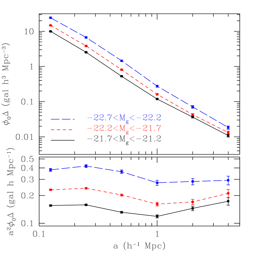
Figure 3: Mean overdensity around red galaxies as a function of proper scale in three different luminosity bins. The top panel shows the quantity $\phi_{0}\Delta$; the bottom panel shows $a^{2}\phi_{0}\Delta$, which is chosen to flatten out the curves so that one can see the fine detail. The deviations from a power-law ${\xi_{\rm is}}$ are clearly visible, as is the luminosity dependence to the clustering. More subtle is the fact that the luminosity dependence is slightly stronger at the smaller scales. The reader is reminded that the $\Delta$ statistic measures the correlation function on scales of $\sim\!1.75a$. Only galaxies in the range $0.20<z<0.36$ have been used. The “1.0” imaging sample is used ($M^{*}-0.5$ to $M^{*}+1.0$).

As stated in §2, measurements at different scales are covariant. We have used our 50 jackknife samples to construct the 6-dimensional covariance matrix for Figure 3 and its “0.4” imaging sample equivalent. With only 50 jackknife samples, the results are noisy, but the covariance between scales appears to reduce from unity by about 50-70% per factor of two in scale (i.e., nearest scales are 50-70% covariant, next nearest are 25-49% covariant, etc.). The lower-luminosity samples, i.e. $-21.7<M_{g}<-21.2$, are more covariant (70%), whereas the more luminous LRGs are less covariant (50%). Widely separated scales, such as in the $0.125h^{-1}{\rm\,Mpc}$ to $2h^{-1}{\rm\,Mpc}$ comparison above, are at most 20% covariant.

Tables 3.2 and 3.2 show mild evidence for a 10% decrease of $\phi_{0}\Delta$ with increasing redshift (in the non-color-selected samples). We see no significant evidence for a change in slope of $\Delta$ versus $L^{1.5}$ as a function of redshift. As stated in §2, both stable clustering and linear theory predict a nearly redshift independent result. Unfortunately, uncertainties in the redshift evolution of the imaging sample currently prevent us from describing the exact evolution of $\phi_{0}\Delta$ and confirming these hypotheses. If the results from the extrapolation of the $z=0.1$ SDSS luminosity-color function (Table 3.2) are correct, then the comoving density of the imaging sample is increasing slightly with redshift, such that the $\phi_{0}\Delta$ for a sample of fixed comoving density would be scaling as $(1+z)^{-2}$. This would argue for some anomaly beyond stable clustering, perhaps caused by some kind of unmodeled evolution. However, it may be that cluster galaxies evolve similarly to our model and that it is the field galaxies that are driving the evolution of the luminosity function (e.g. Lin et al., 1999), in which case stable clustering would predict constant $\phi_{0}\Delta$ regardless of the bulk evolution in $\phi_{0}(z)$. Calibrating our empirical measurement will require more precise modeling of the redshift distribution of SDSS galaxies at these flux levels. In principle, we could measure the differential evolution between different scales, but the predicted variations are smaller than our measurement uncertainties. On the positive side, the insensitivity to redshift validates our averaging $\phi_{0}\Delta$ over galaxies at many redshifts; any deviations from a volume-limited LRG sample (which are minor in any case) would produce negligible biases in $\Delta$.

4.2 Fraction of red galaxies

Figure 4: The fraction of red galaxies in the imaging sample as a function of LRG luminosity for different scales. Each line is a different scale, from $a=0.125h^{-1}{\rm\,Mpc}$ to $4h^{-1}{\rm\,Mpc}$ by factor of two, from top to bottom. A red galaxy is defined as being within $\delta(g-i)$ mag in observed $g-i$ color from the red sequence color at the LRG redshift (see Table 3.2); this classification is not redshift independent and so the fraction of red galaxies is hard to quantify versus redshift. However, because the samples are volume-limited, comparisons between scales and LRG luminosities are well posed. The errors are computed from the variations in the red fraction among the jackknife samples, not from propagation of errors in $\phi_{0}\Delta$. (Upper left) $M^{*}+1.0$ sample for $0.20<z<0.36$. (Upper right) $M^{*}+0.4$ sample for $0.20<z<0.36$. (Lower left) $M^{*}+1.0$ sample for $0.20<z<0.28$. (Lower right) $M^{*}+0.4$ sample for $0.28<z<0.36$.

We define the red fraction as the ratio of $\phi_{0}\Delta$ for our red galaxy imaging sample to that for the full imaging sample. Because $\phi_{0}V\Delta+\phi_{0}V$ really is the average number of galaxies, weighted by $W(r)$, surrounding our LRGs, this ratio of these quantities is the fraction of those galaxies that are red, as defined in §3.3. We neglect the homogeneous term $\phi_{0}V$ because it is negligible at small scales (only 10% of the clustered term at $a=1h^{-1}{\rm\,Mpc}$ and dropping as $a^{2}$ below that), whereas the red fractions at larger scales are close enough to the field values that including the homogeneous term wouldn’t change the ratio appreciably (e.g., for $a=4h^{-1}{\rm\,Mpc}$, the results might drop by 3%).

Figure 3.2 shows the red galaxy fraction as a function of scale and LRG luminosity. The red galaxy fraction is a strong function of scale $a$, as one would expect from the excess of early-type galaxies in dense regions (Abell, 1965; Oemler, 1974; Melnick & Sargent, 1977; Dressler, 1980; Postman & Geller, 1984). We see a slight increase in the red fraction around higher luminosity LRGs, but only on small scales. On scales above 1 Mpc, we do not detect a trend with luminosity. The higher luminosity “0.4” imaging sample has a slightly higher red fraction, as one would expect from the color-magnitude distribution of galaxies.

We display two different redshift bins in the bottom panels of Figure 3.2. The higher redshift bin has a smaller red fraction. While this trend is in the same direction as the conventional wisdom that galaxies are bluer at higher redshift, it is also possible that our selection definition has created a moving target, as discussed in §3.3 One effect that is certainly present is that our $r$-band flux limits select galaxies at bluer rest-frame wavelengths at higher redshift, causing the samples to tilt toward a bluer fraction. In addition, our definition of a “red” galaxy could be redshift dependent due to imperfect modeling of the rest-frame colors. It is interesting to note that the red fractions at the $a=4h^{-1}{\rm\,Mpc}$ scale are only slightly higher than the fractions predicted from the low-redshift SDSS luminosity-color function in Table 3.2. This suggests that at $\sim\!7h^{-1}{\rm\,Mpc}$ ($10h^{-1}{\rm\,Mpc}$ comoving), one has nearly converged back to the field value, despite having chosen the galaxies by their proximity to a LRG.

The top panel of Figure 5 shows the red fraction as a function of scale for 3 redshift bins and the “0.4” imaging sample. Again, the red fraction is redshift dependent. In the bottom panel, we attempt to correct for the simplest effect, namely that lower luminosity blue galaxies can enter the sample at higher redshift simply because of more favorable $k$-corrections. We do this by simply reducing the number of blue galaxies at higher redshift by some fraction $x$ ($x=1$ being no change). If the red fraction at the higher redshift is $f_{2}$, then the fraction $f_{1}$ at the lower redshift, having diluted the blue galaxy density by $x$, will be $f_{1}=(1-x+x/f_{2})^{-1}$. Note that this is not simply a multiplicative scaling in the red fraction. From the model in §3.3 and Table 3.2 in which we extrapolate the low-redshift luminosity-color function without any color evolution, we derive $x=0.86$ (0.75) for $0.28<z<0.36$ ($0.36<z<0.44$) relative to the $0.20<z<0.28$ sample. Applying these corrections, we see that the red fractions at large scales (i.e., the field) are consistent with being independent of redshift. On smaller scales, there is a trend with redshift, suggesting that in regions near LRGs (i.e., high-density regions), galaxies have reddened with time. Strictly speaking, this is the evolution of a population defined by location rather than one that is consistently tagged across time.

We stress again to the reader that variations in the definition of “red” as a function of redshift could still move the curves up or down, so one should not conclude that there is no evolution of the red fraction in the field. These uncertainties should be amenable to better modeling of the galaxy $k$-corrections and luminosity functions. For example, differential luminosity evolution between red and blue galaxies (Lin et al., 1999) could alter the red fraction predictions from Table 3.2. Nevertheless, the conclusion that the evolution of the red fraction is different between regions near LRGs and far from LRGs is robust, as we have used the same definition of “red” at all scales.

Figure 5: (Top panel) The fraction of red galaxies in the imaging sample as a function of scale for different redshift bins. In all cases, only LRGs in the range $-22.2<M_{g}<-21.8$ are used, and the imaging galaxies are from the “0.4” sample. The points with error bars are the measurements with $0.20<z<0.28$, $0.28<z<0.36$, and $0.36<z<0.44$, from top to bottom. (Bottom panel) The same, but the two higher redshift bins have been rescaled according to the model that the blue galaxies are to be diluted by 86% and 75%, respectively. These numbers were determined from extrapolation of the MAIN sample in the absence of any evolution of intrinsic color. The red fractions on larger scales are consistent after this rescaling; the smaller scales show a significant difference.

We also caution against interpreting galaxies near LRGs as necessarily representing a cluster (e.g., mass above $10^{14}\rm M_{\odot}$) population, as not all LRGs live in clusters (e.g., Loh et al., 2003). However, the densities in these regions are high on average, about $16h^{3}{\rm\,Mpc}^{-3}$ for the $a=0.125h^{-1}{\rm\,Mpc}$ case, and so our results will surely bear on the question of differential evolution between high and low density environments (e.g. Hashimoto et al., 1998; Balogh et al., 1999; Margoniner et al., 2001; Lewis et al., 2002; Gomez et al., 2003; de Propris et al., 2004).

5 Discussion

We have demonstrated that the environments of LRGs, as measured by the surrounding overdensity of $L^{*}$ galaxies, varies strongly with luminosity. Across the range from $2.2L^{*}$ to $8.3L^{*}$, the clustering amplitude changes by a factor of 4 on $0.2h^{-1}{\rm\,Mpc}$ scales and a factor of 2 on $7h^{-1}{\rm\,Mpc}$ scales. This trend was clearly seen before (Norberg et al., 2001; Zehavi et al., 2002; Hogg et al., 2003a), but here we use the large volume of the LRG sample to bring this result to very high signal-to-noise ratio. Moreover, the variation of the slope versus luminosity as a function of scale implies that LRGs have a scale-dependent bias that varies with luminosity. Higher luminosity LRGs have even more clustering on sub-Mpc scales than one would project from their clustering on $\sim 5h^{-1}{\rm\,Mpc}$ scales.

The variation of clustering amplitude as a function of LRG luminosity is striking in its strength, and of course these galaxies are already more clustered than less luminous galaxies. This clearly points to a significant change in the masses of the host halos of LRGs as a function of luminosity.

The clustering as a function of scale shows clear deviations from a power law, in a manner quite consistent with the LRG autocorrelation function (Zehavi et al., 2004c) and with less luminous samples (Zehavi et al., 2004a, b). The interpretation in terms of the one-halo and two-halo terms of the halo occupation model (Ma & Fry, 2000; Peacock & Smith, 2000; Seljak, 2000; Scoccimarro et al., 2001; Berlind & Weinberg, 2002) would naturally explain the qualitative structure (Berlind et al., 2003; Magliocchetti & Porciani, 2003; Scranton, 2003; Zehavi et al., 2004a); we will pursue quantitative analyses in future papers. Combining the cross-correlations methods employed here with the LRG and $L^{*}$ galaxy auto-correlations should yield new constraints on the LRG and $L^{*}$ galaxy populations in massive halos.

The fraction of red galaxies as a function of scale and luminosity are qualitatively consistent with the familiar density-morphology relation (Dressler, 1980; Postman & Geller, 1984). Higher luminosity LRGs are surrounded by a slightly larger fraction of red galaxies at sub-Mpc scales.

Tracking redshift evolution is a challenge to any clustering method, as it requires detailed understanding of the evolution of the selection. In our case, this is phrased as the need for a measurement of the number density $\phi_{0}$ of the imaging sample. Redshift evolution of differential effects can still be measured robustly. We find, for example, that the relation of red fraction versus scale changes with redshift, such that the high-density regions near LRGs have reddened more than low-density regions far from LRGs. This result cannot be avoided simply by rescaling the number of blue galaxies, thereby addressing the most obvious gap in our modeling. We intend to pursue this issue further in future work. More generally, with precise modeling of the redshift distribution of the galaxies in the SDSS images, we could recover $\phi_{0}$ and measure the evolution of $\Delta$.

We propose that the scale-dependent clustering of LRGs could serve as a test of the formation theories for these galaxies. In particular, the strong clustering on small scales is a challenge for theories that rely on passive evolution from high redshift, with no environment-dependent evolution of the galaxy. If LRGs sit in only the most massive halos, then they will be highly clustered (Kaiser, 1984; Bardeen et al., 1986; Mo & White, 1996; Sheth, Mo, & Tormen, 2001), but the correlation between their halos’ mass today and their environment at high redshift may not be sufficiently tight to allow the high-redshift environment to dictate today’s luminosity. Processes that enhance the LRG luminosity in situ would loosen these constraints.

More generally, this work highlights the considerable advantage of using cross-correlations between imaging and spectroscopic data sets for the study of the small-scale clustering of rare types of galaxies. On small scales, one is nearly always shot-noise limited, and auto-correlation analyses will suffer two portions of shot noise for rare objects. Cross-correlations with more populous sets of galaxies only incur the shot noise once. Of course, one would expect that the clustering trends are reduced in the cross-correlation, but this is a mild loss of signal compared to the gains in the signal-to-noise ratio. Moreover, for luminous galaxies, acquiring spectroscopic redshifts for the fainter $L^{*}$ companions is doubly challenging, as they are both faint and numerous. Angular cross-correlations therefore allow one to leverage a considerable amount of imaging data. Because the correlations effectively impose a redshift on the imaging data, one can extract rest-frame properties from the imaging set (such as the red fractions presented here) despite not having true redshifts.

We expect that this method could have considerable application to deep wide-field data from the next generation of ground-based surveys or from the Spitzer satellite, as it offers a precise and quantitative measurement of clustering with a minimum of spectroscopic information.

DJE and IZ are supported by grant AST-0098577 from the National Science Foundation. DJE was further supported by an Alfred P. Sloan Research Fellowship.

Funding for the creation and distribution of the SDSS Archive has been provided by the Alfred P. Sloan Foundation, the Participating Institutions, the National Aeronautics and Space Administration, the National Science Foundation, the U.S. Department of Energy, the Japanese Monbukagakusho, and the Max Planck Society. The SDSS Web site is http://www.sdss.org/.

The SDSS is managed by the Astrophysical Research Consortium (ARC) for the Participating Institutions. The Participating Institutions are The University of Chicago, Fermilab, the Institute for Advanced Study, the Japan Participation Group, The Johns Hopkins University, Los Alamos National Laboratory, the Max-Planck-Institute for Astronomy (MPIA), the Max-Planck-Institute for Astrophysics (MPA), New Mexico State University, University of Pittsburgh, Princeton University, the United States Naval Observatory, and the University of Washington.

A Implementation Details

When implementing the summation for the $\Delta_{j}$, it is easy to take account of masks and boundaries as well as to avoid summing over very widely separated pairs. Following Eisenstein (2003), we limit the explicit summation at some $R_{max}$ (we use $10a$) and add the remaining piece

$$\Delta_{outer}={\bar{n}\over\phi_{0}V}\int_{R_{\rm max}}^{\infty}2\pi R\,dR\;[1+{w_{\rm is}}(R)]G(R)$$ (A1)

Here, $\bar{n}$ is the number density of objects from the imaging catalog (selected at the chosen redshift) per unit area on the sky (measured in transverse distance units). The homogeneous term (the 1 in the square brackets) has an easy integral involving $F(R)$, whereas the correlated term can be easily done using a power-law approximation for ${w_{\rm is}}$ and the large-radius expansion for $G(R)$. If ${\xi_{\rm is}}\propto r^{-1-\alpha}$ so that ${w_{\rm is}}\propto r^{-\alpha}$, then we have

$${\bar{n}\over\phi_{0}}{w_{\rm is}}(R)=R{\xi_{\rm is}}(R){\Gamma({\alpha\over 2})\sqrt{\pi}\over\Gamma({\alpha+1\over 2})}$$ (A2)

and so

$$\Delta_{outer}={\bar{n}\over\phi_{0}}{2\pi F({R_{\rm max}})\over V}-{\xi_{\rm is}}({R_{\rm max}}){\Gamma({\alpha\over 2})\sqrt{\pi}\over\Gamma({\alpha+1\over 2})\pi(1+\alpha)}.$$ (A3)

The second term depends on ${\xi_{\rm is}}$, which is what we are trying to find via $\Delta$. However, if the correction is small, then it is a good approximation to keep the shape of ${\xi_{\rm is}}$ fixed while trying to find its amplitude. In this case, the second term becomes

$$\Delta_{outer,clust}=-\Delta{{\xi_{\rm is}}({R_{\rm max}})\over{\xi_{\rm is}}(a)}{\beta\over\pi(1+\alpha)}.$$ (A4)

where

$$\beta={\Gamma({\alpha\over 2})\sqrt{\pi}\over\Gamma({\alpha+1\over 2})}{3\over 2}\sqrt{\pi\over 2}\sqrt{2}^{\alpha}{1\over\Gamma(2-{\alpha\over 2})}$$ (A5)

$\beta=10.49$ for $\alpha=0.75$ and $\beta=3\pi$ for $\alpha=1$.

Hence, to include the effects of the upper limit to the explicit summation, we now have

$$\Delta_{j} = {1\over\phi_{0}V}\left[-2\pi\bar{n}F({R_{\rm max}})+\sum_{k\in\{im\},R_{jk}<{R_{\rm max}}}G(R_{jk})\right]$$ (A6)

$$-\Delta{{\xi_{\rm is}}({R_{\rm max}})\over{\xi_{\rm is}}(a)}{\beta\over\pi(1+\alpha)}$$

We now would average the $\Delta_{j}$ over many spectroscopic objects to estimate $\Delta$. However, note that the last term is just linear in $\Delta$, so we can instead compute

$$\Delta_{j}^{\prime}={1\over\phi_{0}V}\left[-2\pi\bar{n}F({R_{\rm max}})+\sum_{k\in\{im\},R_{jk}<{R_{\rm max}}}G(R_{jk})\right]$$ (A7)

for each object, and then estimate $\Delta$ for any subset as

$$\Delta={\left<\Delta_{j}^{\prime}\right>\over 1+{{\xi_{\rm is}}({R_{\rm max}})\over{\xi_{\rm is}}(a)}{\beta\over\pi(1+\alpha)}}$$ (A8)

where the angle brackets indicate averaging over a subset of spectroscopic objects.

An inner integration limit can be treated the same way, although the integral for the correlated term is different.

$$\Delta_{inner} = {\bar{n}\over\phi_{0}V}\int_{0}^{R_{\rm min}}2\pi R\,dR\;[1+{w_{\rm is}}(R)]G(R)$$ (A10)

$$= {\bar{n}\over\phi_{0}}{2\pi F({R_{\rm min}})\over V}+{2\pi{R_{\rm min}}{\xi_{\rm is}}({R_{\rm min}})\over V}{\Gamma({\alpha\over 2})\sqrt{\pi}\over\Gamma({\alpha+1\over 2})}\times$$

$$\int_{0}^{R_{\rm min}}R\,dR\;G(R)\left({R_{\rm min}}\over R\right)^{\alpha}$$

For the $W(r)$ in equation 6, the second term becomes

$$\Delta_{inner,clust}=\Delta\left({R_{\rm min}}\over a\right)^{5}{{\xi_{\rm is}}({R_{\rm min}})\over{\xi_{\rm is}}(a)}{\beta\over\sqrt{8\pi}(4-\alpha)}.$$ (A11)

Because of the apodization of the window at small radii, this term is quite small, typically of order $({R_{\rm min}}/a)^{3}$. However, other choices of $W(r)$ that have $W(0)\neq 0$ will have larger contributions.

Finally, the same principles apply to masked regions. As described in Eisenstein (2003), it is easy to solve the problem by Monte Carlo by creating a dense set of random points on the sky outside of the survey (i.e., filling the masks and any border regions). We then add to each $\Delta_{j}$ a quantity computed by summing over the random points found within the ${R_{\rm min}}$ to ${R_{\rm max}}$ radial interval, subject to the weighting $G(R)[1+{w_{\rm is}}(R)](\bar{n}/\bar{n}_{random})$, where $\bar{n}_{random}$ is the areal density of the random catalog in the same units of $\bar{n}$. Again, the correlated term can be finessed by approximating ${w_{\rm is}}(R)={w_{\rm is}}(a)(R/a)^{-\alpha}$, as it then becomes

$$\Delta_{mask,clust}={a\over V\bar{n}_{random}}\Delta\beta\sum_{k\in\{ran\}}G(R_{jk})\left(R_{jk}\over a\right)^{-\alpha}$$ (A12)

Hence, in practice, we compute

$$\Delta_{j}^{\prime} = {1\over\phi_{0}V}\left[\sum_{k\in\{im\},R_{jk}<{R_{\rm max}}}G(R_{jk})\right.$$ (A13)

$$+2\pi\bar{n}(F({R_{\rm min}})-F({R_{\rm max}}))$$

$$+\left.{\bar{n}\over\bar{n}_{random}}\sum_{k\in\{ran\},R_{jk}<{R_{\rm max}}}G(R_{jk})\right]$$

and

$$M_{j}={a\beta\over V\bar{n}_{random}}\sum_{k\in\{ran\},R_{jk}<{R_{\rm max}}}G(R_{jk})\left(R_{jk}\over a\right)^{-\alpha}$$ (A14)

For a particular subset of spectroscopic objects, we estimate $\Delta$ as

$$\Delta={\left<\Delta_{j}^{\prime}\right>\over 1-\left<M_{j}\right>+{\beta\over\pi(1+\alpha)}{{\xi_{\rm is}}({R_{\rm max}})\over{\xi_{\rm is}}(a)}-{\beta\over\sqrt{8\pi}(4-\alpha)}\left({R_{\rm min}}\over a\right)^{5}{{\xi_{\rm is}}({R_{\rm min}})\over{\xi_{\rm is}}(a)}}$$ (A15)

Again, $\beta\approx 10$ and $\alpha$ is typically 0.7 to 1. Obviously, one would like to pick ${R_{\rm max}}$ and ${R_{\rm min}}$ so that the corrections in the denominator are minimal; we use ${R_{\rm max}}=10a$, which should be less than 2% correction, and ${R_{\rm min}}=30h^{-1}$ kpc, which is a tiny correction. We exclude any objects for which the mask covered more than 40% of the ${R_{\rm max}}$ circular region, but in practice most objects have very little masking. We find $\left<M_{j}\right>$ to be 1% or less, even for $a=4h^{-1}{\rm\,Mpc}$ with ${R_{\rm max}}=40h^{-1}{\rm\,Mpc}$. For ${R_{\rm max}}=40h^{-1}{\rm\,Mpc}$, about 1/3 of the objects have some fraction of their region masked; this number drops rapidly for smaller ${R_{\rm max}}$.

Our formulae use the flat-sky approximation, which is well-satisfied since the angle on the sky even for the largest ${R_{\rm max}}$ ($40h^{-1}{\rm\,Mpc}$) and closest LRGs is only $5^{\circ}$ and the angles contributing significantly to the integrals are yet smaller. The residuals would be of order $\theta^{2}$, which is $\ll 1$%. We note that it is important to define the flat-sky radius $R$ as $2D\sin(\theta/2)$ for distance $D$ to the LRG and separation angle $\theta$ between the two objects, as this preserves a homogeneous distribution from the sphere to the flat sky and permits the unclustered background to cancel exactly from $\Delta$.

At present, our mask only includes the major boundaries of the survey, not small-scale effects such as bright stars or bad columns. If these masks were uncorrelated with the catalog of spectroscopic objects, then the neglect of these regions would not bias the values of $\Delta$. Of course, the masks and catalogs are correlated. We assess the amount of spurious correlation by using an catalog of M stars as our “spectroscopic” set. We choose reasonably bright, extremely red M stars, as this region of color-magnitude space has essentially no galaxy contaminants that could correlate with the imaging catalog. We place the stars fictitiously at $z=0.3$ and compute the correlations with the galaxies. The results are consistent with zero, with errors that are roughly the same as the errors in the LRG clustering signal. In other words, the neglect of the small-scale mask is less than a 1–$\sigma$ effect for our measurements.

Photometric calibration errors would correlate the spectroscopic LRGs with the imaging catalog, since both samples impose a flux limit, and create a false signal. However, the effect is small. Following equation (A1), we have

$$\phi_{0}V\Delta_{\rm cal}=\bar{n}\int_{0}^{\infty}2\pi R\;dR\;{w_{\rm is}}G(R),$$ (A16)

where ${w_{\rm is}}$ is now the cross-correlation between the two samples due to the calibration error. If ${w_{\rm is}}$ were scale-independent for scales near $a$, as would be the case if the calibration were wrong in patches whose size was much larger than $a$, then this integral would cancel to zero. To avoid cancellation, one must have structure in ${w_{\rm is}}$ near the scale $a$. The function $G(R)$ peaks at 0.8 at $R\approx a$. Conservatively, one would have $\phi_{0}V\Delta_{\rm cal}=\bar{n}\pi a^{2}{w_{\rm is}}(a)$. $\bar{n}\approx 8h^{2}{\rm\,Mpc}^{-2}$ for the “1.0” sample at $z=0.3$, so for $a=1h^{-1}{\rm\,Mpc}$, we have $\phi_{0}V\Delta_{\rm cal}\approx 25{w_{\rm is}}$. The observed $\phi_{0}V\Delta$ exceeds 5 with 3% errors. Hence, we need the calibration-induced ${w_{\rm is}}$ to be less than 0.006. The SDSS rms error in the $r$ band are about 2%, which produces a 6% response in the LRGs (Eisenstein et al., 2001) and a 2% response in the imaging sample. This implies ${w_{\rm is}}=0.0012$, a factor of 5 smaller than required. This is conservative because the actual correlation function from the SDSS calibration errors is a smooth function of scale, i.e., the 2% errors accrue from errors on many patch sizes, which tends to cause the integral in equation (A16) to be smaller. Hence, angular correlations between the samples due to calibration errors are negligibly small for our purpose.

It is worth noting that the deprojection formalism can be applied trivially to spectroscopic auto-correlation applications with the usual projected correlation function

$$w_{p}(R)\equiv 2\int_{-\infty}^{\infty}dZ\;\xi_{red}(\sqrt{Z^{2}+R^{2}}),$$ (A17)

where $\xi_{red}(r)$ is the redshift space correlation function. Defining $\Delta$ as in Equation (1), we have

$$\Delta={1\over V}\int_{0}^{\infty}2\pi R\;dR\;w_{p}(R)G(R)$$ (A18)

Hence, to compute $\Delta$ from an auto-correlation study, there is no need to deproject $w_{p}$ to $\xi_{real}$ and then integrate to $\Delta$.

B Weak Lensing Effects

We argue here that weak lensing magnification effects are small for our analysis, only a $\sim\!1\%$ effect, comparable to our quoted errors in the best cases. The root reasons are simple: our flux limits select $L^{*}$ galaxies at the redshift of the LRG, so the luminosity implied for a target at a redshift high enough to be lensed effectively is much higher, resulting in a low density of potential sources. In more observational terms, at $z=0.3$ we are using $r=20$ galaxies and there are rather few $r=20$ galaxies at $z\gtrsim 0.6$ on the sky. Furthermore, the scales we are studying ($>0.2h^{-1}{\rm\,Mpc}$) are large compared to the Einstein radius of an LRG or even a reasonable cluster.

Mathematically, we consider magnification patterns of the form $(R/R_{E})^{-1}$, where $R_{E}$ is a constant. This would generate an angular correlation proportional to $R^{-1}$, with the amplitude depending on the cosmological distances and the slope of the luminosity function.

For example, summing over source redshifts, one could write the contribution to $\Delta$ as

$$\phi_{0}\Delta_{WL} = {1\over V}\int 2\pi R\,dR\;G(R)\int_{z_{LRG}}^{\infty}dz\;\phi(z)$$ (B19)

$$\times\left[D_{M}(z)\over D_{M}(z_{LRG})\right]^{2}(\alpha-1)\left(R_{E}(z)\over R\right)$$

where $z$ is the distance along the line of sight (not redshift), $R$ is the transverse distance across the line of sight, $D_{M}(z)$ is the cosmological proper motion distance, $\phi(z)$ is the comoving density of galaxies passing the selection at the LRG redshift, $\alpha$ is the logarithmic slope of the cumulative luminosity function, and $R_{E}(z)$ is the Einstein radius (in distance, not angle) for that source redshift. The ratio of $D_{M}$ enters because of the volume per solid angle, and the $\alpha-1$ is the familiar competition between magnification of sources and dilution of source density (Turner et al., 1984).

The equation can be simplified by noting that equations (10), (A2), and

$$\Delta={\bar{n}\over\phi_{0}V}\int_{0}^{\infty}2\pi R\,dR\;{w_{\rm is}}(R)G(R)$$ (B20)

[see eq. (A1)] imply that

$${1\over V}\int 2\pi R\,dR\;G(R)\left(R_{0}\over R\right)={R_{0}\over 3\pi a^{2}}$$ (B21)

for the $W(r)$ in equation (6). This means that the weak lensing contribution to $\Delta$ is

$$\Delta_{WL}={1\over 3\pi a^{2}}\int_{z_{LRG}}^{\infty}dz\;{\phi(z)\over\phi_{0}}\left[D_{M}(z)\over D_{M}(z_{LRG})\right]^{2}(\alpha-1)R_{E}(z).$$ (B22)

One could do a careful integration using a luminosity function, but here we will merely estimate. $R_{E}$ is small unless the sources are well behind the lens. Characteristically, we would have $z\approx 2z_{LRG}$ and $D_{M}(z)\approx 2D_{M}(z_{LRG})$. The luminosity threshold will rise as the square of the luminosity distance, which is $(1+z)D_{M}$, in addition to any $k$ corrections, so we would typically have the luminosity threshold increased by about a factor of 5–10. This suggests $\phi(z)\approx 0.01\phi_{0}$. We assume $\alpha-1\approx 1$. The line of sight interval would characteristically be $1000h^{-1}{\rm\,Mpc}$. We conservatively take $R_{E}=20$ kpc, which is already cluster sized ($6^{\prime\prime}$ radius) and would correspond to 10% magnification ratios at $1^{\prime}$ (e.g., Bartelmann & Schneider, 2001; Benítez et al., 2001; Jain et al., 2003). Putting these together suggests $\Delta_{WL}\sim 0.1{\rm\,Mpc}^{2}/a^{2}$, whereas our measured $\Delta$ values are 100 times larger.

The calculation for magnification of the LRG by foreground galaxies is analogous and gives a similar estimate. Here the problem is that the foreground galaxies are well below $L^{*}$ and hence are poor lenses. The volume and path lengths are also less favorable.

We therefore estimate the weak lensing effects at 1-2%. While not important for this work, weak lensing could be an issue for some applications of the cross-correlation method, particularly for studies involving cross-correlation to sub-$L^{*}$ galaxies or to objects with favorable $k$-corrections at high redshifts (e.g. sub-millimeter galaxies).

Table 2:

Fits to Overdensities versus Luminosity
$a$ ($h^{-1}$ Mpc) Redshift^a $L_{back}$^b Color^c $L_{LRG}$^d $\phi_{0}V\Delta(L_{ref})$^e Slope^f $\chi^{2}$^g 0.125 $0.20<z<0.36$ 1.0 $-21.2$ 1.082(13) 0.110(5) 6.8 0.125 $0.20<z<0.28$ 1.0 $-21.2$ 1.100(21) 0.120(8) 10.2 0.125 $0.28<z<0.36$ 1.0 $-21.2$ 1.073(16) 0.108(6) 15.0 0.125 $0.20<z<0.36$ 1.0 $g-i$ $-21.2$ 0.742(9) 0.132(5) 6.7 0.125 $0.20<z<0.28$ 1.0 $g-i$ $-21.2$ 0.803(14) 0.145(8) 7.9 0.125 $0.28<z<0.36$ 1.0 $g-i$ $-21.2$ 0.704(10) 0.125(6) 10.5 0.25 $0.20<z<0.36$ 1.0 $-21.2$ 2.214(26) 0.118(5) 7.8 0.25 $0.20<z<0.28$ 1.0 $-21.2$ 2.287(39) 0.131(8) 4.4 0.25 $0.28<z<0.36$ 1.0 $-21.2$ 2.159(34) 0.111(6) 6.8 0.25 $0.20<z<0.36$ 1.0 $g-i$ $-21.2$ 1.336(16) 0.141(5) 11.4 0.25 $0.20<z<0.28$ 1.0 $g-i$ $-21.2$ 1.482(25) 0.149(8) 7.1 0.25 $0.28<z<0.36$ 1.0 $g-i$ $-21.2$ 1.248(20) 0.137(7) 12.2 0.5 $0.20<z<0.36$ 1.0 $-21.2$ 3.64(6) 0.130(7) 13.2 0.5 $0.20<z<0.28$ 1.0 $-21.2$ 3.77(8) 0.137(10) 10.9 0.5 $0.28<z<0.36$ 1.0 $-21.2$ 3.56(8) 0.126(9) 12.9 0.5 $0.20<z<0.36$ 1.0 $g-i$ $-21.2$ 2.046(30) 0.133(7) 24.8 0.5 $0.20<z<0.28$ 1.0 $g-i$ $-21.2$ 2.25(5) 0.140(10) 11.0 0.5 $0.28<z<0.36$ 1.0 $g-i$ $-21.2$ 1.914(39) 0.131(9) 17.1 1.0 $0.20<z<0.36$ 1.0 $-21.2$ 6.42(15) 0.090(9) 7.0 1.0 $0.20<z<0.28$ 1.0 $-21.2$ 6.72(22) 0.089(12) 11.1 1.0 $0.28<z<0.36$ 1.0 $-21.2$ 6.22(18) 0.090(12) 7.0 1.0 $0.20<z<0.36$ 1.0 $g-i$ $-21.2$ 3.17(7) 0.099(8) 11.0 1.0 $0.20<z<0.28$ 1.0 $g-i$ $-21.2$ 3.39(10) 0.106(11) 5.0 1.0 $0.28<z<0.36$ 1.0 $g-i$ $-21.2$ 3.03(8) 0.093(11) 9.5 2.0 $0.20<z<0.36$ 1.0 $-21.2$ 15.1(4) 0.058(10) 14.1 2.0 $0.20<z<0.28$ 1.0 $-21.2$ 15.1(6) 0.084(14) 7.5 2.0 $0.28<z<0.36$ 1.0 $-21.2$ 15.2(6) 0.046(13) 13.7 2.0 $0.20<z<0.36$ 1.0 $g-i$ $-21.2$ 6.64(14) 0.059(8) 10.4 2.0 $0.20<z<0.28$ 1.0 $g-i$ $-21.2$ 7.03(22) 0.068(12) 11.2 2.0 $0.28<z<0.36$ 1.0 $g-i$ $-21.2$ 6.45(18) 0.053(10) 6.5 4.0 $0.20<z<0.36$ 1.0 $-21.2$ 36.4(15) 0.047(13) 8.0 4.0 $0.20<z<0.28$ 1.0 $-21.2$ 37.4(20) 0.082(18) 10.1 4.0 $0.28<z<0.36$ 1.0 $-21.2$ 35.7(18) 0.024(16) 7.7 4.0 $0.20<z<0.36$ 1.0 $g-i$ $-21.2$ 15.3(4) 0.041(9) 7.3 4.0 $0.20<z<0.28$ 1.0 $g-i$ $-21.2$ 17.4(6) 0.061(12) 12.2 4.0 $0.28<z<0.36$ 1.0 $g-i$ $-21.2$ 14.0(5) 0.022(12) 6.6 NOTES.—^a The redshift range of the LRG sample. ^b The minimum luminosity of the imaging galaxies in magnitudes below $M^{*}$. The maximum luminosity is always $M^{*}-0.5$. This table presents the “1.0” sample. ^c Marked with $g-i$ if imaging galaxies have been required to be within $\delta(g-i)$ mag in observed $g-i$ color of the red sequence at the LRG redshift. ^d The minimum $M_{g}$ of the LRGs used in the fit. ^e The value of the best-fit linear relation of $\phi_{0}V\Delta$ versus $(L/L^{*})^{1.5}$, evaluated at $3.3L^{*}$ for the $M_{g}<-21.2$ sample and $4.5L^{*}$ for the $M_{g}<-21.8$ sample. These values were picked so that the errors on the slope and intercept of the best-fit line are nearly independent. The errors on the last digits are given in parenthesis. We use $M_{g}^{*}=-20.35$. ^f The slope of the best-fit line and its error, both divided by the value in the previous column to give a reasonable normalization (but one that is different between this table and Table 3.2). ^g $\chi^{2}$ of the data with respect to the best-fit line. Samples with $M_{g}<-21.2$ have 15 luminosity bins and hence 13 degrees of freedom. Samples with $M_{g}<-21.8$ have 9 luminosity bins and hence 7 degrees of freedom.

Table 3:

$a$ ($h^{-1}$ Mpc)	Redshift	$L_{back}$	Color	$L_{LRG}$	$\phi_{0}V\Delta(L_{ref})$	Slope	$\chi^{2}$
0.125	$0.20<z<0.44$	0.4		$-21.8$	0.637(13)	0.065(7)	7.9
0.125	$0.20<z<0.28$	0.4		$-21.8$	0.645(27)	0.085(18)	2.7
0.125	$0.28<z<0.36$	0.4		$-21.8$	0.673(20)	0.063(12)	7.2
0.125	$0.36<z<0.44$	0.4		$-21.8$	0.616(20)	0.068(11)	5.1
0.125	$0.20<z<0.44$	0.4	$g-i$	$-21.8$	0.468(8)	0.071(7)	4.7
0.125	$0.20<z<0.28$	0.4	$g-i$	$-21.8$	0.530(21)	0.093(17)	3.3
0.125	$0.28<z<0.36$	0.4	$g-i$	$-21.8$	0.481(13)	0.072(11)	2.9
0.125	$0.36<z<0.44$	0.4	$g-i$	$-21.8$	0.433(11)	0.068(10)	2.5
0.25	$0.20<z<0.44$	0.4		$-21.8$	1.314(23)	0.084(7)	6.0
0.25	$0.20<z<0.28$	0.4		$-21.8$	1.45(5)	0.091(15)	3.8
0.25	$0.28<z<0.36$	0.4		$-21.8$	1.355(38)	0.067(11)	3.5
0.25	$0.36<z<0.44$	0.4		$-21.8$	1.219(35)	0.098(11)	3.3
0.25	$0.20<z<0.44$	0.4	$g-i$	$-21.8$	0.870(15)	0.090(7)	7.9
0.25	$0.20<z<0.28$	0.4	$g-i$	$-21.8$	1.013(35)	0.103(15)	3.4
0.25	$0.28<z<0.36$	0.4	$g-i$	$-21.8$	0.911(24)	0.088(10)	5.6
0.25	$0.36<z<0.44$	0.4	$g-i$	$-21.8$	0.782(21)	0.084(10)	7.2
0.5	$0.20<z<0.44$	0.4		$-21.8$	2.21(5)	0.083(8)	4.8
0.5	$0.20<z<0.28$	0.4		$-21.8$	2.47(9)	0.092(17)	0.8
0.5	$0.28<z<0.36$	0.4		$-21.8$	2.37(8)	0.075(14)	5.2
0.5	$0.36<z<0.44$	0.4		$-21.8$	2.00(8)	0.091(14)	5.3
0.5	$0.20<z<0.44$	0.4	$g-i$	$-21.8$	1.342(28)	0.098(8)	10.4
0.5	$0.20<z<0.28$	0.4	$g-i$	$-21.8$	1.63(6)	0.106(17)	3.1
0.5	$0.28<z<0.36$	0.4	$g-i$	$-21.8$	1.41(5)	0.103(13)	10.0
0.5	$0.36<z<0.44$	0.4	$g-i$	$-21.8$	1.18(4)	0.097(11)	10.7
1.0	$0.20<z<0.44$	0.4		$-21.8$	3.68(12)	0.067(11)	12.2
1.0	$0.20<z<0.28$	0.4		$-21.8$	4.00(25)	0.075(21)	4.9
1.0	$0.28<z<0.36$	0.4		$-21.8$	3.92(19)	0.080(20)	4.6
1.0	$0.36<z<0.44$	0.4		$-21.8$	3.39(18)	0.043(18)	12.1
1.0	$0.20<z<0.44$	0.4	$g-i$	$-21.8$	1.98(5)	0.068(9)	8.2
1.0	$0.20<z<0.28$	0.4	$g-i$	$-21.8$	2.34(11)	0.076(19)	1.8
1.0	$0.28<z<0.36$	0.4	$g-i$	$-21.8$	2.09(9)	0.098(19)	3.4
1.0	$0.36<z<0.44$	0.4	$g-i$	$-21.8$	1.78(7)	0.044(12)	4.2
2.0	$0.20<z<0.44$	0.4		$-21.8$	8.19(33)	0.064(12)	11.9
2.0	$0.20<z<0.28$	0.4		$-21.8$	8.7(6)	0.078(24)	6.9
2.0	$0.28<z<0.36$	0.4		$-21.8$	7.9(5)	0.076(26)	9.2
2.0	$0.36<z<0.44$	0.4		$-21.8$	8.1(5)	0.056(20)	8.2
2.0	$0.20<z<0.44$	0.4	$g-i$	$-21.8$	4.07(11)	0.055(9)	10.1
2.0	$0.20<z<0.28$	0.4	$g-i$	$-21.8$	4.57(24)	0.069(21)	5.8
2.0	$0.28<z<0.36$	0.4	$g-i$	$-21.8$	4.19(19)	0.062(18)	4.2
2.0	$0.36<z<0.44$	0.4	$g-i$	$-21.8$	3.77(16)	0.040(14)	4.2
4.0	$0.20<z<0.44$	0.4		$-21.8$	20.2(13)	0.031(17)	5.2
4.0	$0.20<z<0.28$	0.4		$-21.8$	24.3(19)	0.061(27)	3.5
4.0	$0.28<z<0.36$	0.4		$-21.8$	20.5(20)	-0.003(28)	5.0
4.0	$0.36<z<0.44$	0.4		$-21.8$	18.4(17)	0.035(27)	6.6
4.0	$0.20<z<0.44$	0.4	$g-i$	$-21.8$	9.29(35)	0.027(11)	5.4
4.0	$0.20<z<0.28$	0.4	$g-i$	$-21.8$	12.0(7)	0.055(20)	3.4
4.0	$0.28<z<0.36$	0.4	$g-i$	$-21.8$	9.0(5)	0.009(19)	3.8
4.0	$0.36<z<0.44$	0.4	$g-i$	$-21.8$	8.5(5)	0.021(18)	5.8

NOTES.—As Table 3.2, but for the higher luminosity “0.4” imaging sample, which allows us to use higher redshift LRGs if we restrict to high luminosity LRGs.

References

- Abazajian et al. (2003) Abazajian, K., et al., 2003, AJ, 126, 2081
- Abazajian et al. (2004) Abazajian, K., et al., 2004, AJ, 128, 502
- Abell (1965) Abell, G.O., 1965, ARA&A, 3, 1
- Balogh et al. (1999) Balogh, M.L., Morris, S.L., Yee, H.K.C., Carlberg, R.G., & Ellingson, E., 1999, ApJ, 527, 54
- Bardeen et al. (1986) Bardeen, J.M., Bond, J.R., Kaiser, N., & Szalay, A.S., 1986, ApJ, 304, 15
- Bartelmann & Schneider (2001) Bartelmann, M., & Schneider, P., 2001, Physics Reports, 340, 291
- Baugh & Efstathiou (1993) Baugh, C.M., & Efstathiou, G. 1993, MNRAS, 265, 145
- Benítez et al. (2001) Benítez, N., Sanz, J.L., Martínez-Gonz/’alez, E., 2001, MNRAS, 320, 241
- Benoist et al. (1998) Benoist, C., Cappi, A., da Costa, L. N., Maurogordato, S., Bouchet, F. R., & Schaeffer, R. 1998, ApJ, 514, 563
- Berlind & Weinberg (2002) Berlind, A. A., & Weinberg, D. H. 2002, ApJ, 575, 587
- Berlind et al. (2003) Berlind, A. A., Weinberg, D. H., Benson, A. J., Baugh, C. M., Cole, S., et al. 2003, ApJ, 593, 1
- Blanton et al. (2002) Blanton, M.R., et al., 2002, ApJ, 594, 186; astro-ph/0209479
- Blanton et al. (2003a) Blanton, M.R., Lupton, R.H., Maley, F.M., Young, N., Zehavi, I., Loveday, J., 2003a, AJ, 125, 2276
- Blanton et al. (2003b) Blanton, M.R., et al., 2003b, ApJ, 592, 819
- Blanton et al. (2003c) Blanton, M.R., et al., 2003c, ApJ, in press; astro-ph/0310453
- Bower et al. (1992) Bower, R.G., Lucey, J.R., & Ellis, R.S. 1992, MNRAS, 254, 601
- Broadhurst et al. (1988) Broadhurst, T.J., Ellis, R.S., Shanks, T., 1988, MNRAS, 235, 827
- Brown, Webster & Boyle (2000) Brown, M. J. I., Webster, R. L., & Boyle, B. J. 2000, MNRAS, 317, 782
- Budavari et al. (2003) Budavari, T., et al., 2003, ApJ, 595, 59
- Butcher & Oemler (1978) Butcher, H, & Oemler, A., 1978, ApJ, 219, 18
- Butcher & Oemler (1984) Butcher, H, & Oemler, A., 1984, ApJ, 285, 426
- Carlberg et al. (2001) Carlberg, R. G., Yee, H. K. C., Morris, S. L., Lin, H., Hall, P. B., Patton, D. R., Sawicki, M., & Shepherd, C. W. 2001, ApJ, 563, 736
- Davis & Geller (1976) Davis, M., & Geller, M. J. 1976, ApJ, 208, 13
- Davis et al. (1978) Davis, M., Geller, M.J., & Huchra, J., 1978, ApJ, 221, 1
- de Propris et al. (2004) de Propris, R., et al. (the 2dFGRS Team), 2004, MNRAS, 351, 125
- Dodelson & Gaztañaga (2000) Dodelson, S., & Gaztañaga, E. 2000, MNRAS, 312, 774
- Dressler (1980) Dressler, A. 1980, ApJ, 236, 351
- Dressler & Gunn (1983) Dressler, A, & Gunn, J.E., 1983, ApJ, 270, 7
- Drory et al. (2004) Drory, N., Bender, R., Feulner, G., Hopp, U., Maraston, C., Snigula, J., & Hill, G. J., 2004, ApJ, 608, 742
- Eisenstein & Zaldarriaga (2001) Eisenstein, D.J., & Zaldarriaga, M. 2001, ApJ, 546, 2
- Eisenstein et al. (2001) Eisenstein, D.J., et al., 2001, AJ, 122, 2267
- Eisenstein (2003) Eisenstein, D.J., 2003, ApJ, 586, 718
- Faber (1973) Faber, S.M. 1973, ApJ, 179, 731
- Fall & Tremaine (1977) Fall, S.M., & Tremaine, S., 1977, ApJ, 216, 682
- Ferguson & Sandage (1991) Ferguson, H.C., Sandage, A. 1991, AJ, 101, 765
- Fontana et al. (2004) Fontana, A., et al., 2004, A&A, 424, 23
- Fukugita et al. (1996) Fukugita, M., Ichikawa, T., Gunn, J.E., Doi, M., Shimasaku, K., & Schneider, D.P., 1996, AJ, 111, 1748
- Glazebrook et al. (2004) Glazebrook, K., et al., 2004, Nature, 430, 181
- Gomez et al. (2003) Gomez, P. et al. 2003, ApJ, 584, 210
- Guzzo et al. (1997) Guzzo, L., Strauss, M. A., Fisher, K. B., Giovanelli, R., & Haynes, M. P. 1997, ApJ, 489, 37
- Gunn et al. (1998) Gunn, J.E., et al., 1998, AJ, 116, 3040
- Hamilton (1988) Hamilton, A. J. S. 1988, ApJ, 331, L59
- Hashimoto et al. (1998) Hashimoto, Y., Oemler, A., Lin, H., & Tucker, D.L., 1998, ApJ, 499, 589
- Hoessel et al. (1980) Hoessel, J.G., Gunn, J.E., Thuan, T.X., 1980, ApJ, 241, 486
- Hogg et al. (2001) Hogg, D.W., Finkbeiner, D.P., Schlegel, D.J., & Gunn, J.E. 2001, AJ, 122, 2129
- Hogg et al. (2003a) Hogg, D.W., et al., 2003, ApJ, 585, L5
- Hubble (1936) Hubble, E.P. 1936, The Realm of the Nebulae (Oxford University Press: Oxford), 79
- Hubble & Humason (1931) Hubble, E., & Humason, M. L., 1931, ApJ, 74, 43
- Jain et al. (2003) Jain, B., Scranton, R., & Sheth, R.K., 2003, MNRAS, 345, 62
- Jones et al. (1991) Jones, L.R., Fong, R., Shanks, T., Ellis, R.S., & Peterson, B.A., 1991, MNRAS, 249, 481
- Kaiser (1984) Kaiser, N. 1984, ApJ, 284, L9
- Lavery & Henry (1986) Lavery, R.J., & Henry, J.P., 1986, ApJ, 304, L5
- Lewis et al. (2002) Lewis, I. et al. 2002, MNRAS, 334, 673
- Lilje & Efstathiou (1988) Lilje, P.B., Efstathiou, G., 1988, MNRAS, 231, 635
- Lilly et al. (1991) Lilly, S.J., Cowie, L.L., Gardner, J.P. 1991, ApJ, 369, 79
- Lilly et al. (1996) Lilly, S. J., Le Fevre, O., Hammer, F., & Crampton, David 1996, ApJ, 460, 1
- Lin et al. (1999) Lin, H., Yee, H. K. C., Carlberg, R. G., Morris, S. L., Sawicki, M., Patton, D. R., Wirth, G., & Shepherd, C. W., 1999, ApJ, 518, 533
- Loh et al. (2003) Loh, Y. S., et al. 2003, Ph.D. thesis, Princeton University
- Lorrimer et al. (1994) Lorrimer, S.J., Frenk, C.S., Smith, R.M., White, S.D.M., Zaritsky, D., 1994, MNRAS, 269, 696
- Loveday et al. (1995) Loveday, J., Maddox, S. J., Efstathiou, G., & Peterson, B. A. 1995, ApJ, 442, 457
- Loveday (1997) Loveday, J., ApJ, 489, 29 (1997)
- Lupton et al. (2001) Lupton, R., Gunn, J.E., Ivezić, Z., Knapp, G.R., Kent, S., & Yasuda, N. 2001, in ASP Conf. Ser. 238, Astronomical Data Analysis Software and Systems X, ed. F. R. Harnden, Jr., F. A. Primini, and H. E. Payne (San Francisco: Astr. Spc. Pac.); astro-ph/0101420
- Ma & Fry (2000) Ma, C., & Fry, J. N. 2000, ApJ, 543, 503
- Madau et al. (1996) Madau, P.; Ferguson, H. C.; Dickinson, M. E.; Giavalisco, M.; Steidel, C. C.; Fruchter, A. 1996, MNRAS, 283, 1388
- Madgwick et al. (2003) Madgwick, D. S. et al. 2003, MNRAS, 344, 847
- Magliocchetti & Porciani (2003) Magliocchetti, M., & Porciani, C. 2003, MNRAS, 346, 186
- Margoniner et al. (2001) Margoniner, V.E., de Carvalho, R.R., Gal, R.R., & Djorgovski, S.G., 2001, apj, 548, L143
- McCarthy et al. (2001) McCarthy, P.J., et al., 2001, ApJ, 560, L131
- Melnick & Sargent (1977) Melnick, J., & Sargent, W. L. W. 1977, ApJ, 215, 401
- Metcalfe et al. (1991) Metcalfe, N., Shanks, T., Fong, R., & Jones, L.R., 1991, MNRAS, 249, 498
- Mo & White (1996) Mo, H. J., & White, S. D. M. 1996, MNRAS, 282, 1096
- Norberg et al. (2001) Norberg, P., et al. 2001, MNRAS, 328, 64
- Norberg et al. (2002) Norberg, P., et al. 2002, MNRAS, 332, 827
- Oemler (1974) Oemler, A. 1974, ApJ, 194, 1
- Park et al. (1994) Park, C., Vogeley, M. S., Geller, M. J., & Huchra, J. P. 1994, ApJ, 431, 569
- Peacock & Smith (2000) Peacock, J. A., & Smith, R. E. 2000, MNRAS, 318, 1144
- Peebles (1980) Peebles, P.J.E., 1980, The Large-Scale Structure of the Universe (Princeton: Princeton Univ. Press), § 71
- Phillipps (1985) Phillipps, S., 1985, MNRAS, 212, 657
- Phillipps & Shanks (1987) Phillipps, S., Shanks, T., 1987, MNRAS, 227, 115
- Pier et al. (2003) Pier, J. R., et al. 2003, AJ, 125, 1559
- Postman & Geller (1984) Postman, M., & Geller, M. J. 1984, ApJ, 281, 95
- Postman & Lauer (1995) Postman, M. & Lauer, T.R., 1995, ApJ, 440, 28
- Sandage (1972) Sandage, A., 1972, ApJ, 178, 1
- Saunders et al. (1992) Saunders, W., Rowan-Robinson, M., & Lawrence, A. MNRAS, 258, 134 (1992)
- Schlegel et al. (1998) Schlegel, D. J., Finkbeiner, D. P., & Davis, M. 1998, ApJ, 500, 525
- Schneider et al. (1983) Schneider, D.P., Gunn, J.E., Hoessel, J.G., 1983, ApJ, 264, 337
- Scoccimarro et al. (2001) Scoccimarro, R., Sheth, R. K., Hui, L., & Jain, B. 2001, ApJ, 546, 20
- Scranton (2003) Scranton, R. 2003, MNRAS, 339, 410
- Seljak (2000) Seljak, U. 2000, MNRAS, 318, 203
- Sheth, Mo, & Tormen (2001) Sheth, R. K., Mo, H. J., & Tormen, G. 2001, MNRAS, 323, 1
- Smith, Tucker et al. (2002) Smith, J. A., Tucker, D. L. et al. 2002, AJ, 123, 2121
- Stoughton et al. (2002) Stoughton, C. et al. 2002, AJ, 123, 485
- Strauss et al. (2002) Strauss, M.A., et al., 2002, AJ, 124, 1810
- Tyson (1988) Tyson, J.A., 1988, AJ, 96, 1
- Turner et al. (1984) Turner, E.L., Ostriker, J.P., & Gott, J.R., 1984, ApJ, 284, 1
- Vader & Sandage (1991) Vader, J.P., Sandage, A. 1991, ApJ, 379, L1
- Verde et al. (2002) Verde, L., et al. 2002, MNRAS, 335, 432
- Visvanathan & Sandage (1977) Visvanathan, N., & Sandage, A. 1977, ApJ, 216, 214
- von Zeipel (1908) von Zeipel, H., 1908, Ann. d’Obs. Paris, 25, 229
- White, Tully, & Davis (1988) White, S. D. M., Tully, R. B., & Davis, M. 1988, ApJ, 333, L45
- Willmer, da Costa & Pellegrini (1998) Willmer, C. N. A., da Costa, L. N., & Pellegrini, P. S. 1998, AJ, 115, 869
- Yee & Green (1987) Yee, H.K.C., & Green, R.F. 1987, ApJ, 319, 28
- York et al. (2000) York, D.G., et al., 2000, AJ, 120, 1579
- Zehavi et al. (2002) Zehavi, I., Blanton, M. R., Frieman, J. A., Weinberg, D. H., Mo, H. J., et al. 2002, ApJ, 571, 172, [Z02]
- Zehavi et al. (2004a) Zehavi, I., et al., 2004a, ApJ, 608, 16
- Zehavi et al. (2004b) Zehavi, I., et al. 2004b, ApJ, submitted
- Zehavi et al. (2004c) Zehavi, I., et al., 2004c, ApJ, submitted
- Zwicky et al. (1968) Zwicky, F., Herzog, E., Wild, P., Karpowicz, M., & Kowal, C., 1961-1968, Catalog of Galaxies and of Clusters of Galaxies, Vols. 1-6, (Pasadena: California Institute of Technology)