The Clustering of Extragalactic Extremely Red Objects

Abstract

We have measured the angular and spatial clustering of 671 $K<18.40$, $R-K>5$ Extremely Red Objects (EROs) from a $0.98~{}{\rm deg}^{2}$ sub-region of the NOAO Deep Wide-Field Survey (NDWFS). Our study covers nearly 5 times the area and has twice the sample size of any previous ERO clustering study. The wide field of view and $B_{W}RIK$ passbands of the NDWFS allow us to place improved constraints on the clustering of $z\sim 1$ EROs. We find the angular clustering of EROs is slightly weaker than in previous measurements, and $\omega(1^{\prime})=0.25\pm 0.05$ for $K<18.40$ EROs. We find no significant correlation of ERO spatial clustering with redshift, apparent color or absolute magnitude, although given the uncertainties, such correlations remain plausible. We find the spatial clustering of $K<18.40$, $R-K>5$ EROs is well approximated by a power-law, with $r_{0}=9.7\pm 1.1~{}h^{-1}{\rm Mpc}$ in comoving coordinates. This is comparable to the clustering of $\sim 4L^{*}$ early-type galaxies at $z<1$, and is consistent with the brightest EROs being the progenitors of the most massive ellipticals. There is evidence of the angular clustering of EROs decreasing with increasing apparent magnitude, when NDWFS measurements of ERO clustering are combined with those from the literature. Unless the redshift distribution of $K\gtrsim 20$ EROs is very broad, the spatial clustering of EROs decreases from $r_{0}=9.7\pm 1.1~{}h^{-1}{\rm Mpc}$ for $K<18.40$ to $r_{0}\sim 7.5~{}h^{-1}{\rm Mpc}$ for $K\gtrsim 20$ EROs.

1 Introduction

The evolution of galaxy clustering is a prediction of hierarchical models of galaxy and structure formation (e.g., Kauffmann et al., 1999; Benson et al., 2001; Somerville et al., 2001). Hierarchical models for a concordance cosmology predict little or no evolution of the clustering of $\gtrsim L^{*}$ red galaxies at $z<2$. Precise measurements of galaxy clustering at $z\sim 1$ can therefore test the predictions of these models.

Extremely Red Objects (EROs; Elston, Rieke, & Rieke, 1988; McCarthy, Persson, & West, 1992; Hu & Ridgway, 1994; Dey, Spinrad, & Dickinson, 1995) could be the progenitors of local ellipticals (e.g., Spinrad et al., 1997). Roughly 80% of $K_{S}<18.7$ EROs have spectra with the absorption features of old stellar populations (Yan, Thompson & Soifer, 2004) and $\sim 50\%$ of $K\lesssim 22$ EROs have early-type morphologies (Moriondo, Cimatti, & Daddi, 2000; Stiavelli & Treu, 2001; Moustakas et al., 2004). Some EROs contain super-massive black holes, as $\sim 15\%$ of EROs contain an obscured Active Galactic Nucleus which can be detected by deep X-ray surveys (Alexander et al., 2002; Roche, Dunlop, & Almaini, 2003). A direct test of the relationship between $z\sim 1$ EROs and the most massive local ellipticals is to compare the spatial clustering of the two populations.

Previous constraints on the spatial correlation function of EROs, summarized in Table 1, are provided by pencil-beam surveys with $\lesssim 0.2~{}{\rm deg}^{2}$ areal coverage each. Individual structures comprised of EROs can have sizes comparable to the field of view of these surveys (e.g., Daddi et al., 2000), and small surveys do not sample representative volumes of the Universe for highly clustered objects (e.g., Somerville et al., 2004). At $z\sim 1$, the transverse comoving distance spanned by previous ERO studies is $\lesssim 20~{}h^{-1}{\rm Mpc}$, which is much smaller than the size of individual structures observed in the present-day Universe. Spatial clustering measurements derived from the angular correlation function depend on ERO redshift distribution models. Previous angular clustering studies were unable to verify their model redshift distributions, as complete spectroscopic samples of EROs were unavailable. Previous ERO spatial clustering measurements have large uncertainties and possibly large (and sometimes unaccounted for) systematic errors.

In this paper, we present a measurement of the clustering of EROs using $B_{W}RIK$ imaging of a $0.98~{}{\rm deg}^{2}$ subset of the NOAO Deep Wide-Field Survey (NDWFS). The large area of our study provides a more representative volume than previous studies. The $B_{W}RIK$ passbands of the NDWFS allow us to constrain the ERO redshift distribution with photometric redshifts and their uncertainties. We also use photometric redshifts to select EROs as a function of luminosity and redshift. We use ERO spectroscopic redshifts to verify the accuracy of our photometric redshifts and we compare our estimate of the ERO redshift distribution with spectroscopic redshift distributions from the literature.

The structure of the paper is as follows. In §2 we provide a brief description of the NDWFS imaging and catalogs from which the $K<18.40$ ERO sample was selected. We discuss our estimates of ERO photometric redshifts, and provide a comparison of ERO photometric and spectroscopic redshifts in §3. The selection of the ERO sample and ERO number counts are discussed in §4. In §5, we describe the techniques used to measure the angular and spatial correlation functions. The angular and spatial clustering of EROs, as a function of apparent magnitude, apparent color, absolute magnitude, and redshift are discussed in §6. We discuss the implications of our results in §7 and summarize the paper in §8.

2 The NOAO Deep Wide-Field Survey

The NDWFS is a multiband ($B_{W},R,I,K$) survey of two $\approx 9.3~{}{\rm deg}^{2}$ high Galactic latitude fields with the CTIO $4{\rm m}$, KPNO $4{\rm m}$, and KPNO $2.1{\rm m}$ telescopes (Jannuzi & Dey, 1999). A thorough description of the optical and $K$-band observing strategy and data reduction will be provided by Jannuzi et al. and Dey et al. (both in preparation). This paper utilizes $0.98~{}{\rm deg}^{2}$ of $B_{W}RIK$ data in the Boötes field. $B_{W}RI$ imaging and catalogs for the entire NDWFS Boötes field became available from the NOAO Science Archive on 22 October 2004. $K$-band imaging and catalogs for approximately half of the Boötes field are also available from this archive.

We generated object catalogs using SExtractor $2.3.2$ (Bertin & Arnouts, 1996), run in single-image mode in a similar manner to Brown et al. (2003). At faint magnitudes, detections in the different bands were matched if the centroids were within $1^{\prime\prime}$ of each other. At bright magnitudes, detections in the different bands were matched if the centroids were within an ellipse defined using the second order moments of the light distribution of the object. Throughout this paper we use SExtractor MAG_AUTO magnitudes (which are similar to Kron total magnitudes; Kron, 1980), due to their small uncertainties and systematic errors at faint magnitudes. Our clustering measurements are not particularly sensitive to how we measure ERO photometry, and the clustering of EROs selected with $4^{\prime\prime}$ diameter aperture photometry is only marginally weaker than the clustering of EROs selected with MAG_AUTO photometry.

We determined the completeness as a function of magnitude by adding artificial objects to copies of the data and recovering them with SExtractor. To approximate $z\sim 1$ galaxies, the artificial objects have an intrinsic profile with a full width at half maximum of $0.5^{\prime\prime}$, which was then convolved with a Moffat profile model of the seeing. The $50\%$ completeness limits vary within the sample area in the ranges of $26.0<B_{W}<26.7$, $24.8<R<25.6$, $23.6<I<25.2$ and $18.6<K<18.7$.

Regions surrounding saturated stars were removed from the catalog to exclude (clustered) spurious objects detected in the wings of the point spread function. We excluded regions where the root-mean-square of the sky noise in the $K$-band data was $20\%$ higher than the mean, as the depth of these regions is significantly less than the mean depth across the field. While it is plausible that smaller variations in the sky noise could alter the measured clustering of the faintest EROs, our main conclusions remain unchanged if we exclude $K>18.15$ EROs from the sample.

We used SExtractor’s star-galaxy classifier to remove objects from the galaxy catalog which had a stellarity of $>0.7$ in 2 or more bands brighter than $B_{W}<23.8$, $R<22.8$, and $I<21.4$. At fainter magnitudes we do not use the star-galaxy classification and correct the angular correlation function for the estimated stellar contamination of the sample. We do not use the $K$-band for star-galaxy classification as there are image quality variations across the $K$-band image stacks. We estimated stellar contamination of the galaxy sample using the same technique as Brown et al. (2003), where the stellar number counts were assumed to be a power-law and the distribution of stellar colors does not change with magnitude at $R\gtrsim 21$. The contamination of the ERO sample (§4) by stars is estimated to be $\sim 2\%$, and the conclusions of this paper remain unaltered unless stellar contamination is higher than $15\%$.

3 Photometric Redshifts

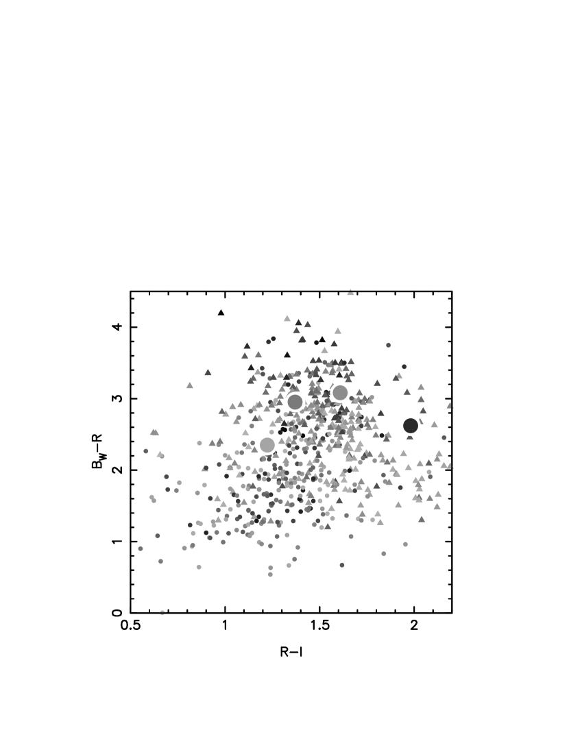
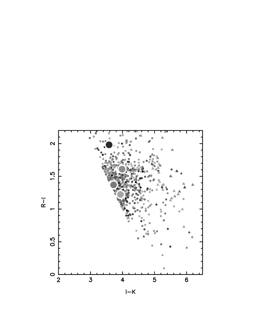
Photometric redshifts were determined for all objects with $I$ and $K$-band detections. We provide a brief overview of the photometric redshifts here and refer the reader to our earlier study of $0.3<z<0.9$ red galaxy clustering in the NDWFS (Brown et al., 2003) for a more detailed description of the photometric redshift code. To model galaxy spectral energy distributions (SEDs), we used PEGASE2 evolutionary synthesis models (Fioc & Rocca-Volmerange, 1997) with exponentially declining star formation rates ($\tau$ models) and $z=0$ ages of $12~{}{\rm Gyr}$ (formation $z\approx 4$). The effect of $E(B-V)=0.04$ dust reddening with $R_{V}=3.1$, comparable to estimates for $0<z<1$ early-type galaxies (Falco et al., 1999), was included in the $\tau$ models. In Brown et al. (2003), we used models with solar metallicity at $z=0$, which resulted in small systematic underestimates of galaxy redshifts. Simple solar metallicity $\tau$ models underestimate the UV luminosity of galaxies (e.g., Donas, Milliard, & Laget, 1995), so in this work we let the metallicity of the models be a function of $\tau$. This has the effect of slightly increasing the UV flux of the model SEDs. We verified the accuracy of the photometric redshifts at $z<1$ with 89 $M_{R}<-19-5{\rm log}h$ galaxies with rest-frame $B_{W}-R>1.05$ and spectroscopic redshifts. After decreasing the metallicity of the models, the photometric redshifts of these red galaxies did not have significant systematic errors. We note, however, that the UV flux in galaxies can also be increased by the presence of young stars or by altering the properties of the dust extinction; our approach is merely a proxy for correcting any systematic effects in our photometric redshifts and is not meant to be interpreted as justifying sub-solar metallicities in the red galaxy population. We use these solar and sub-solar $\tau$ models throughout the remainder of the paper. Color-tracks for 2 of the models are shown in Figure 1. For comparison, we also show two ultra-luminous infrared galaxy (ULIRG) templates from Devriendt, Guiderdoni, & Sadat (1999), which have bluer $B_{W}-R$ colors than the $\tau$ models at $z\sim 1$.

Photometric redshifts were estimated by finding the minimum value of $\chi^{2}$ as a function of redshift, spectral type ($\tau$), and luminosity. For objects not detected in the $R$ or $B_{W}$-bands, we estimated the probability of a non-detection using the completeness estimates discussed in §2. As the model SEDs do not account for the observed width of the galaxy locus, we increased the photometric uncertainties for the galaxies by $0.05$ magnitudes (added in quadrature). To improve the accuracy of the photometric redshifts, the estimated redshift distribution of galaxies as a function of spectral type and apparent magnitude was introduced as a prior. The 2dF Galaxy Redshift Survey (2dFGRS) luminosity functions for different spectral types (Madgwick et al., 2002), with spectral evolution given by the $\tau$-models, were used to estimate the redshift distributions.

We tested the reliability of the photometric redshifts with simulated galaxies and real galaxies with spectroscopic redshifts. Simulated galaxies were generated using the PEGASE2 $\tau$ models. The simulated data consisted of $K<18.40$ galaxies with $0.6~{}{\rm Gyr}\leq\tau\leq 15~{}{\rm Gyr}$ in the redshift range $0<z\leq 5$ and luminosity range $0.01<L^{*}\leq 100$. The simulated object photometry was scattered using the estimated uncertainties, thus mimicking what would be present in the real catalogs. We tested the accuracy of the photometric redshifts with a few spectroscopic redshifts and $B_{W}RIK$ photometry for EROs in the NDWFS Boötes field.

A comparison of our photometric and spectroscopic redshifts for EROs is shown in Figure 2. We discuss the selection criteria for the EROs in §4. The simulated galaxies in the left panel of Figure 2 have $1\sigma$ uncertainties of $\simeq 8\%$. For galaxies with SEDs similar to the PEGASE2 $\tau$ models, our procedure should yield accurate photometric redshifts. There are 4 NDWFS $K<18.40$ EROs with spectroscopic redshifts. As shown in the right hand panel of Figure 2, real EROs in the NDWFS exhibit a $1\sigma$ scatter of $\sim 20\%$ between the photometric and spectroscopic redshifts. There are more outliers than would be expected if the $\tau$ models reproduced the variety of ERO SEDs. For comparison, GOODS obtains ERO photometric redshifts with accuracies of $\sim 5\%$ (Mobasher et al., 2004), as they have photometry and upper limits in more bands ($U^{\prime}UBB_{435}VV_{606}RIi_{775}z_{850}JHK_{S}$). The accuracy of photometric redshifts is a complex function of redshift, SED and apparent magnitude. The accuracy of the ERO photometric redshifts could not be extrapolated from $z<1$ red galaxy photometric redshifts, which can have uncertainties of $<10\%$ (e.g., Brown et al., 2003). The accuracy of ERO photometric redshifts can not, and should not, be extrapolated from other samples of galaxies, such as samples selected by apparent magnitude only or from the Hubble Deep Fields (HDFs). Though our ERO photometric redshifts can only be considered approximations, they provide a good estimate of the ERO redshift distribution (see §5).

4 The Extremely Red Object Sample

We selected EROs with the $R-K>5$ criterion (e.g., Elston, Rieke, & Rieke, 1988; Daddi et al., 2000; Roche et al., 2002), though redder color cuts are sometimes used in the literature (e.g., Hu & Ridgway, 1994; Dey et al., 1999). We have limited the sample to $K<18.40$ EROs, to reduce the effects of completeness variations across the survey area on the measured clustering. As shown in Figure 3, the percentage of EROs increases from $\simeq 0\%$ of the total galaxy counts at $K<16$ to $\simeq 8\%$ at $K\simeq 18.4$.

Contamination of the ERO sample by other galaxies could significantly alter the measured correlation function. At the magnitude limit of our sample, the uncertainty in the $R-K$ color is $\simeq 0.25$ magnitudes. For the distribution of galaxy colors shown in Figure 3, and assuming Gaussian photometric uncertainties, approximately 6% of the $K<18.40$ ERO sample is contamination by $R-K<4.75$ galaxies. Even if $R-K<4.75$ galaxies were completely (and implausibly) unclustered, the amplitude of the $R-K>5$ angular correlation function would only be decreased by 12%. Contamination by $4.75<R-K<5.00$ galaxies could be as high as 22% in the $K<18.40$ ERO sample. This would significantly alter our results if the clustering of galaxies is a very strong function of color at $R-K\sim 5$. However, as discussed in §6.2, we do not see evidence of this within our dataset. Malmquist (1920) bias does increase the observed number of EROs. If we assume the ERO number counts in Table 2 are a good approximation of the true ERO number counts, then the contribution of Malmquist bias to the NDWFS counts is $\lesssim 8\%$. This would alter the measured clustering if ERO angular clustering is an extremely strong function of apparent magnitude.

We assume the bulk of our sample consists of galaxies with red stellar populations. The colors of dusty starbursts are predicted to differ significantly from galaxies with red stellar populations. As shown in Figure 4, 77% of the NDWFS ERO sample has $R-I>1.15$, which is redder than the Devriendt, Guiderdoni, & Sadat (1999) non-evolving ULIRG templates shown in Figure 1. Our assumption that most $K<18.40$ EROs have red stellar populations is also consistent with the conclusions of Yan, Thompson & Soifer (2004), who find 86% of $K_{S}<18.7$ EROs have the absorption features of old stellar populations.

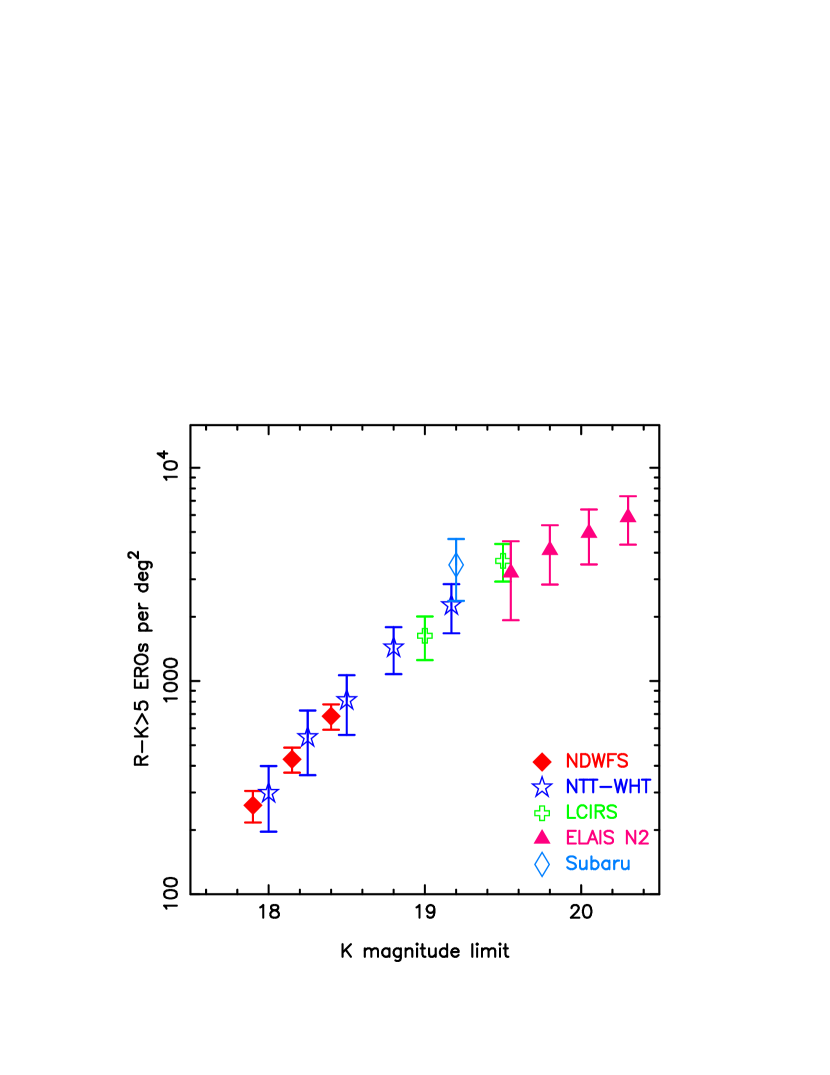
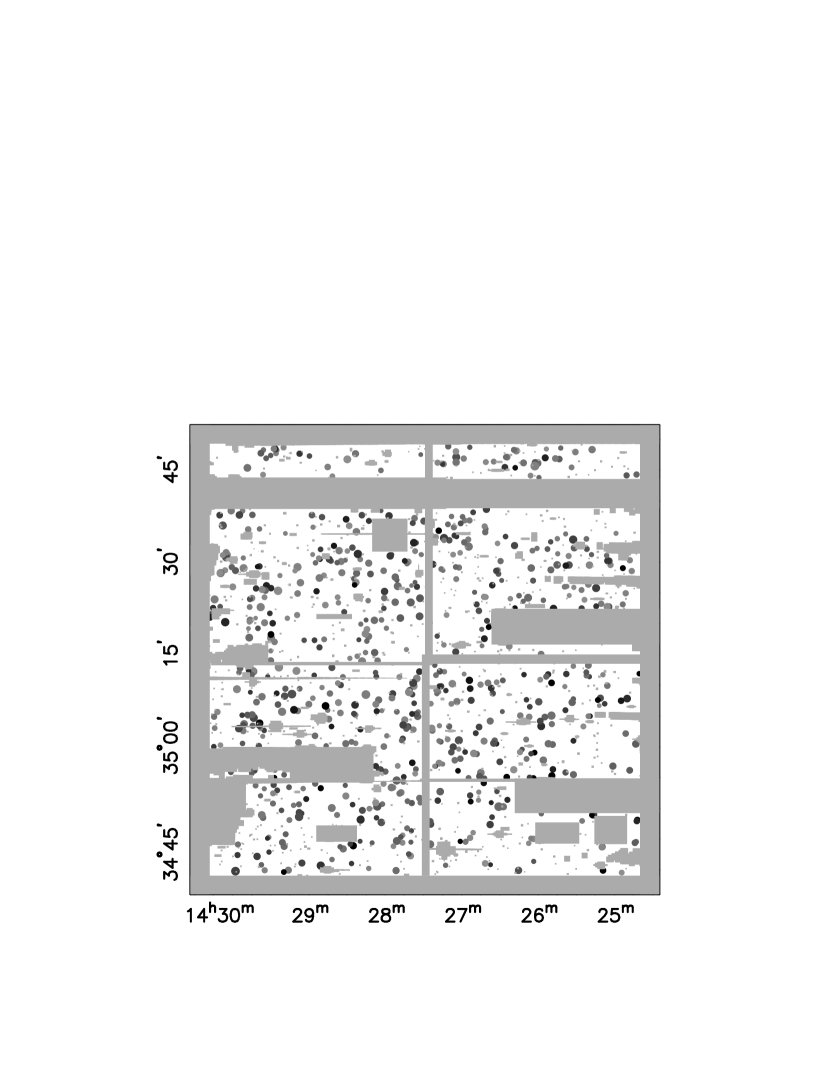
The final sample consists of 671 objects, of which 318 are detected in the $B_{W}$-band and 635 are detected in the $R$-band. The $K<18.4$ EROs have photometric redshifts in the range $0.8\leq z\leq 3.0$, with the median of the distribution at $z\simeq 1.18$. Only 5 of the 671 $K<18.4$ EROs have photometric redshifts of $z>2$. ERO number counts as a function of $K$-band limiting magnitude are provided in Table 2 and Figure 5, along with results from previous surveys. We evaluated the uncertainties of the sky surface density, for the NDWFS and previous work, using the method discussed by Efstathiou et al. (1991), which includes the contribution of large-scale structure. The contribution of clustering to the uncertainties is typically several times larger than uncertainties determined by Poisson statistics. For our $K<18.4$ ERO sample, accounting for the clustering increases the $1\sigma$ uncertainty from 5% to 20%! We note that the uncertainties quoted by some studies do not include this contribution (e.g., Roche et al., 2002; Miyazaki et al., 2003; Roche, Dunlop, & Almaini, 2003). The distribution of the ERO sample on the plane of the sky is shown in Figure 6. ERO surveys of $\sim 0.1~{}{\rm deg}^{2}$ often have individual structures with sizes comparable to the field of view (e.g., Daddi et al., 2000). While clustering and voids are evident in Figure 6, there are no obvious $\sim 0.5^{\circ}$ structures or gradients in the distribution of EROs in our sample.

5 The Correlation Function

We determined the angular correlation function using the Landy & Szalay (1993) estimator:

$$\hat{\omega}(\theta)=\frac{DD-2DR+RR}{RR}$$ (1)

where $DD$, $DR$, and $RR$ are the number of galaxy-galaxy, galaxy-random and random-random pairs at angular separation $\theta\pm\delta\theta/2$. The pair counts were determined in logarithmically spaced bins between $10^{\prime\prime}$ and $0.7^{\circ}$.

We employed the same methodology as Brown et al. (2003) to generate random object catalogs, correct for the integral constraint (Groth & Peebles, 1977), and estimate the covariance of the $\hat{\omega}(\theta)$ bins (using the technique of Eisenstein & Zaldarriaga, 2001). The random object catalog contains 100 times the number of objects as the ERO catalog, so $DR$ and $RR$ are renormalized accordingly.

The angular correlation function was assumed to be a power-law given by

$$\omega(\theta)=\omega(1^{\prime})\left(\frac{\theta}{1^{\prime}}\right)^{1-\gamma}$$ (2)

where $\gamma$ is a constant. This is a good approximation of the observed galaxy spatial correlation function from the 2dFGRS and Sloan Digital Sky Survey (SDSS) on scales of $\lesssim 10~{}h^{-1}{\rm Mpc}$ (Norberg et al., 2001, 2002; Zehavi et al., 2002). Throughout this paper we assume $\gamma=1.87$, the approximate value of $\gamma$ for $z<0.15$ red galaxies from the 2dFGRS and SDSS surveys. For a $\gamma=1.87$ power-law, the integral constraint for this study was approximately $6\%$ of the amplitude of the correlation function at $1^{\prime}$. Pair counts and the estimate of the angular correlation function (including the integral constraint correction) for $R-K>5.0$ and $R-K>5.5$ EROs are presented in Table 3.

The spatial correlation function was obtained using the Limber (1954) equation;

$$\omega(\theta)=\int^{\infty}_{0}\frac{dN}{dz}\left[\int^{\infty}_{0}\xi(r(\theta,z,z^{\prime}),z)\frac{dN}{dz^{\prime}}dz^{\prime}\right]dz\left/\left(\int^{\infty}_{0}\frac{dN}{dz}dz\right)^{2}\right.$$ (3)

where $\frac{dN}{dz}$ is the redshift distribution without clustering, $\xi$ is the spatial correlation function and $r(\theta,z,z^{\prime})$ is the comoving distance between two objects at redshifts $z$ and $z^{\prime}$ separated by angle $\theta$ on the sky. The spatial correlation function was assumed to be a power law given by

$$\xi(r,z)=[r/r_{0}(z)]^{-\gamma}.$$ (4)

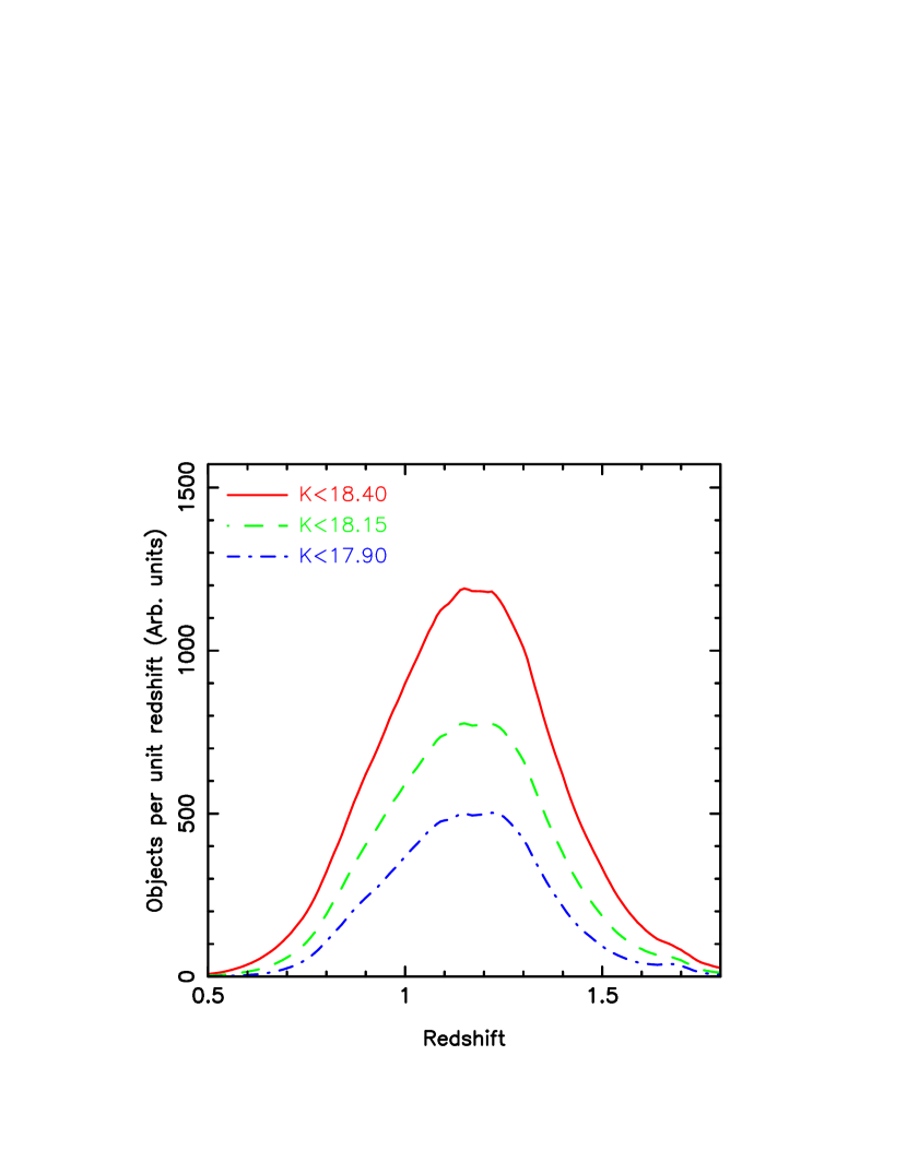
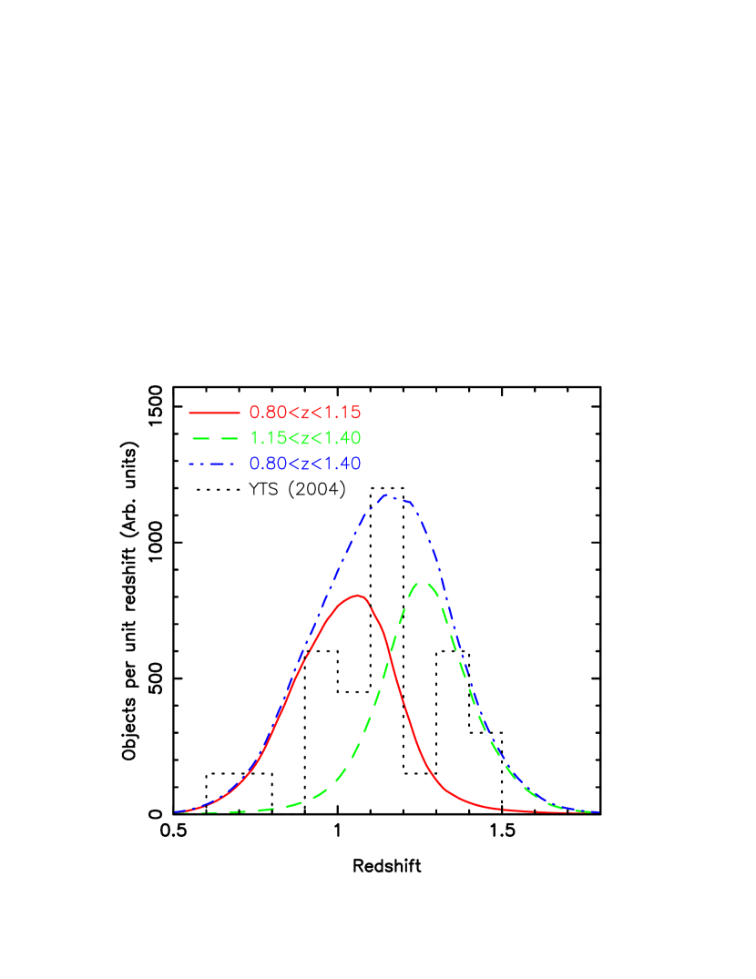
We estimated the redshift distribution for the sample by summing the redshift likelihood distributions of the individual galaxies in each subsample. Model redshift distributions for subsamples selected by apparent magnitude and photometric redshift are shown in Figure 7. While the individual photometric redshifts are not especially accurate, they do include information provided by the observed ERO photometry and are likely to provide a fair approximation of the ERO redshift distribution. Redshift distribution models which only reproduce the apparent ERO number counts and local galaxy luminosity functions (e.g., Daddi et al., 2001; Roche et al., 2002; Roche, Dunlop, & Almaini, 2003) have fewer constraints and may have larger systematic errors. The estimated median redshift of the $K<18.40$ EROs is 1.18, which is almost identical to the spectroscopic median redshift of 24 $K_{S}<18.7$ EROs from Yan, Thompson & Soifer (2004). The median redshift is also similar to $K_{S}<18.5$ EROs in the K20 spectroscopic sample (Cimatti et al., 2002, A. Cimatti 2003, private communication).

6 The clustering of EROs

We measured the angular and spatial correlation functions for a series of apparent magnitude, apparent color, absolute magnitude, and redshift bins. A power-law of the form $\omega(\theta)=A\theta^{1-\gamma}$ was fitted to the data with $\gamma$ fixed to $1.87$. Much larger imaging surveys, including the completed NDWFS Boötes and Cetus fields, will have sufficient area to accurately measure $\gamma$. When parameterizing the power-law fits, we use $\omega(1^{\prime})$ instead of $\omega(1^{\circ})$ as it depends less on the assumed value of $\gamma$. Using $\gamma=1.80$ instead of $\gamma=1.87$ increases $\omega(1^{\prime})$ by $\simeq 10\%$ and $\omega(1^{\circ})$ by $\simeq 35\%$. The best-fit values of $r_{0}$ do depend on the assumed value of $\gamma$, but for the NDWFS ERO sample, changing $\gamma$ from $1.87$ to $1.80$ increases $r_{0}$ by only $\simeq 10\%$. Measurements of $\omega(1^{\prime})$ for EROs as a function of $K$-band limiting magnitude from our study and the literature are summarized in Table 2. Angular correlation functions for apparent magnitude limited samples are also plotted in Figure 8. Estimates of $\omega(1^{\prime})$ and $r_{0}$ for each of the NDWFS subsamples are presented in Table 4 and discussed in §6.1 to §6.4.

6.1 Clustering as a function of apparent magnitude

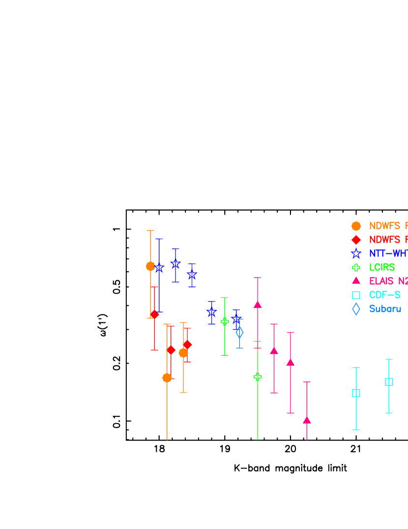
The amplitude of the angular correlation function for a series of apparent magnitude limited samples is presented in Figure 9 and Table 2, along with estimates from the literature. While our $K<18.4$ sample has a larger volume and more objects than previous studies, our uncertainties are comparable to the published uncertainties of many previous studies. This is due to our inclusion of the covariance when fitting a power-law to the data. Our estimates of the amplitude of the angular correlation function are $\sim 2\sigma$ lower than the smaller $K_{S}<18.4$ ERO samples from Daddi et al. (2000). Within our sample we do not see a significant change in the angular clustering amplitude with apparent magnitude, but this is not unexpected as we span a small range of apparent magnitudes.

The first section of Table 4 provides an estimate of $r_{0}$ for EROs as a function of apparent limiting magnitude. While the NDWFS $r_{0}$ values are accurate to $\sim 15\%$, each apparent magnitude bin spans a large range of redshift and absolute magnitude. As $r_{0}$ is correlated with luminosity in other galaxy samples (e.g., Giavalisco & Dickinson, 2001; Norberg et al., 2002; Zehavi et al., 2002; Brown et al., 2003), a correlation between $r_{0}$ and apparent magnitude might be expected. We do not observe a significant correlation within the NDWFS, but our uncertainties are too large to rule out such a correlation.

Combining published ERO samples provides spatial clustering measurements over a broad magnitude range. However, it is not possible to directly compare the published $r_{0}$ measurements of different ERO samples (Table 1), as different authors use different models of the ERO redshift distribution. Different studies also estimate the uncertainties of the angular correlation function and $r_{0}$ using different techniques. In Table 3, we present the NDWFS pair counts for the $R-K>5.0$ and $R-K>5.5$ $K<18.40$ ERO angular correlation functions, so other researchers can apply their techniques for estimating the correlation function to our data. Poisson statistics underestimate the uncertainties of the correlation function on large-scales, where object pair counts are high and the uncertainties of the correlation function are dominated by large-scale structure. The uncertainties of clustering measurements from deep pencil-beam surveys should be larger than those of the NDWFS, and the large scatter of $K>19$ ERO clustering measurements shown in Figure 9 may reflect this.

If we assume the published best-fit values of the amplitude of the angular correlation are correct, then the angular clustering of EROs does decrease with increasing limiting magnitude. We find $\omega(1^{\prime})=0.25\pm 0.05$ for $K<18.40$ EROs while Roche, Dunlop, & Almaini (2003) find $\omega(1^{\prime})\sim 0.13$ for $K<22$ EROs. Unless the redshift distribution of faint EROs is very broad, the spatial clustering of EROs is decreasing with increasing apparent magnitude. Several studies to measure $r_{0}\sim 10~{}h^{-1}{\rm Mpc}$ for faint EROs (Roche et al., 2002; Daddi et al., 2003; Miyazaki et al., 2003; Roche, Dunlop, & Almaini, 2003), but their model redshift distributions contain more high redshift objects than the GOODS $K_{S}<20.1$ ERO photometric redshift distribution (Moustakas et al., 2004). If $\omega(1^{\prime})\simeq 0.13$ for faint EROs and the GOODS photometric redshifts are accurate, then $r_{0}$ decreases from $9.7\pm 1.1~{}h^{-1}{\rm Mpc}$ for $K<18.40$ to $r_{0}\sim 7.5~{}h^{-1}{\rm Mpc}$ for $K\gtrsim 20$ EROs. Red galaxies at $z<1$ have a comparable range of $r_{0}$ values (e.g., Norberg et al., 2002; Zehavi et al., 2002; Brown et al., 2003) and their spatial clustering is correlated with absolute magnitude. The current measurements of ERO clustering are consistent with EROs being the progenitors of local red galaxies.

6.2 Clustering as a function of apparent color

We present the clustering of $R-K>5.0$ and $R-K>5.5$ EROs in Figure 9 and Table 4. We find the angular and spatial clustering of $R-K>5.5$ galaxies does not differ significantly from the remainder of the sample. Low redshift galaxies may have a bimodal distribution of clustering properties as a function of color (Budavári et al., 2003). This could be due to the bimodal distribution of galaxy colors at low redshift, or a bimodality of the clustering properties of galaxies as a function of star formation rate. If the clustering is bimodal at all redshifts, we would not expect a correlation between clustering and color within a red galaxy sample. We do not see a correlation of clustering with color but a larger sample with improved photometric redshifts is required so accurate spatial clustering measurements can be performed as a function of rest-frame color.

6.3 Clustering as a function of absolute magnitude

The clustering of EROs as a function of absolute magnitude is presented in Table 4. We have determined the absolute magnitudes (without evolution corrections) of the EROs using the best-fit $\tau$-model SED. As shown in Figure 2, ERO photometric redshifts can have large uncertainties and our ERO absolute magnitudes are, at best, approximations. The two absolute magnitude bins are approximately volume limited samples with the same photometric redshift range. Both absolute magnitude bins are extremely luminous, and contain EROs approximately 4 times brighter than the local value of $L^{*}$ ($M^{*}_{K}=-23.44\pm 0.03$; Cole et al., 2001). We do not see a significant correlation between luminosity and $r_{0}$ within the sample. The correlation between galaxy luminosity and clustering is only seen unambiguously in $z<1$ samples (e.g., 2dFGRS and SDSS) which contain a factor of $\gtrsim 10$ more galaxies than the NDWFS ERO sample. A strong correlation between ERO luminosity and spatial clustering remains plausible, and may be detected with an analysis of the complete NDWFS.

6.4 Clustering as a function of redshift

We measured the clustering of EROs within the sample with two photometric redshift bins, $0.80<z<1.15$ and $1.15<z<1.40$. We exclude EROs beyond these redshift ranges, as they contribute less than $10\%$ of the total $K<18.40$ ERO number counts. The results are presented in Table 4 and Figure 10. We do not observe significant evolution of $r_{0}$ with redshift within the ERO sample. However, our uncertainties are large and the redshift distributions of the two samples overlap, so they are not entirely independent.

7 Discussion

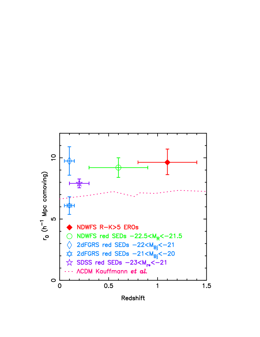
The clustering of $0.80<z<1.40$, $K<18.40$ EROs is well approximated by a power law with $r_{0}=9.6\pm 1.0~{}h^{-1}{\rm Mpc}$ and $\gamma$ fixed at $1.87$. As EROs are thought to be the progenitors of local ellipticals, it is useful to compare the clustering measurements of these populations. In the 2dFGRS, the spatial correlation function increases from $r_{0}=6.10\pm 0.72~{}h^{-1}{\rm Mpc}$ for $\simeq 2L^{*}$ red galaxies to $r_{0}=9.74\pm 1.16~{}h^{-1}{\rm Mpc}$ for $\simeq 4L^{*}$ red galaxies (Norberg et al., 2002). Other $z<1$ surveys, including the NDWFS, measure comparable spatial clustering for red galaxies (e.g., Willmer, da Costa, & Pellegrini, 1998; Budavári et al., 2003; Brown et al., 2003). It is not unreasonable to assume the brightest EROs are the progenitors of the $\simeq 4L^{*}$ red galaxies in the local Universe, as the comoving spatial clustering of the two populations is comparable. However, this assumes models predicting little or no evolution of the $\gtrsim L^{*}$ galaxy correlation function (e.g., Kauffmann et al., 1999; Benson et al., 2001) are valid.

If $K<18.40$ EROs are the progenitors of the most luminous local red galaxies, fainter EROs could the progenitors of $\sim L^{*}$ red galaxies. Several previous studies of fainter EROs find they are very strongly clustered, with $r_{0}\sim 10~{}h^{-1}{\rm Mpc}$ (Roche et al., 2002; Daddi et al., 2003; Miyazaki et al., 2003; Roche, Dunlop, & Almaini, 2003). This is much stronger than the clustering of local $L^{*}$ red galaxies, where $r_{0}\simeq 6h^{-1}{\rm Mpc}$ (Norberg et al., 2002; Zehavi et al., 2002). However, the ERO spatial clustering measurements could be subject to large, and possibly systematic, errors. Several of these measurements use model redshift distributions which are primarily constrained by the local galaxy luminosity function and faint galaxy number counts (Daddi et al., 2001; Roche et al., 2002; Roche, Dunlop, & Almaini, 2003). Other model redshift distributions use unverified photometric redshifts (Miyazaki et al., 2003) or redshifts which could only be verified with galaxies other than EROs (Firth et al., 2002). As shown in Figure 9, the angular clustering of EROs does decrease with increasing apparent magnitude. Unless the redshift distribution of $K\gtrsim 20$ EROs is very broad, the spatial clustering of $K\gtrsim 20$ EROs is weaker than the spatial clustering of $K<18.40$ EROs.

While $K<18.40$ EROs may be the progenitors of most luminous local ellipticals, our spatial clustering measurement should be treated with some caution. Our ERO sample spans broad ranges of redshift and absolute magnitude ($-27.9\lesssim M_{K}-5{\rm log}h\lesssim-23.9$). The luminosity and density evolution of EROs and red galaxies at $z<1$ has not been accurately determined. The PEGASE $\tau$ models predict $\sim 0.8$ magnitudes of luminosity evolution at $z<1$, so EROs would be the progenitors to $\simeq 2L^{*}$ red galaxies. If this were the case, the spatial correlation function would be decreasing with decreasing redshift, which is unphysical. The uncertain luminosity and density evolution of EROs limits the use of $>L^{*}$ EROs to measure the evolution of the galaxy spatial correlation function.

Current ERO spatial clustering measurements, including our study, have large uncertainties and may be subject to systematic errors. We will significantly reduce the random uncertainties of ERO clustering measurements when we analyze the entire NDWFS Boötes field. The uncertainties and systematic errors of our photometric redshifts will be accurately determined as we obtain more spectroscopic redshifts. We will also improve the photometric redshifts for EROs by using NDWFS, FLAMINGOS (Gonzalez et al., 2004), and Spitzer Space Telescope data. We will then be able to accurately measure the spatial clustering of EROs as a function of luminosity, color, and redshift.

8 Summary

We have measured the clustering of 671 $K<18.40$ EROs with $0.98~{}{\rm deg}^{2}$ subset of the NDWFS. This study covers an area nearly 5 times larger and has twice the sample size of any previous ERO clustering study. The angular clustering of $K<18.40$, $R-K>5.0$ EROs is well described by a power-law with $\omega(1^{\prime})=0.25\pm 0.05$ and $\gamma=1.87$. Using a model of the ERO redshift distribution derived from photometric redshifts, we find the spatial clustering of $K<18.40$ EROs is given by $r_{0}=9.7\pm 1.0~{}h^{-1}{\rm Mpc}$ comoving. Within our study, we detect no significant correlations between ERO clustering and apparent magnitude, apparent color, absolute magnitude, or redshift. However, our uncertainties are large and such correlations may exist. When combined with data from other studies, there is evidence of the angular clustering of EROs decreasing with increasing apparent magnitude. Unless the redshift distribution of $K\gtrsim 20$ EROs is very broad, the spatial clustering of EROs decreases with increasing apparent magnitude. As the uncertainties and systematic errors of current ERO spatial clustering measurements are large, they do not yet provide strong tests of models of structure evolution and galaxy formation.

Figure 1: Color-color diagrams of the PEGASE2 $\tau$-models and non-evolving templates of Arp 220 and IRAS 05189-2524 (Devriendt, Guiderdoni, & Sadat, 1999). The $R-K=5$ selection criterion for EROs is shown in the right-hand panel. Dots mark $z=0$, $1$, $2$, and $3$ on the model tracks. For clarity, the redshift range shown is restricted to $0\leq z\leq 3$ and we have not plotted $\tau$-models bluer than the ERO color cut.

Figure 2: A comparison of $K<18.40$ $R-K>5.0$ ERO photometric and spectroscopic redshifts for simulated and real data. Dotted diagonal lines show the measured $\pm 1\sigma$ uncertainties of the photometric redshifts. Simulated EROs, generated using the $\tau$-models with photometric noise added, are shown in the left-hand panel. On the right are real EROs with spectroscopic redshifts. For clarity only a third of the simulated galaxies are plotted. The measured $1\sigma$ uncertainties of the photometric redshifts for real EROs is $\sim 20\%$.

Figure 3: The color-magnitude diagram and the number of $K<18.40$ galaxies as a function of $R-K$ color. The $R-K=5$ selection criterion is marked with dashed lines. Only 25% of all the galaxies have been plotted in the color-magnitude diagram and $R-K$ lower limits are denoted by triangles. The $R$ magnitude limits vary across the $0.98~{}{\rm deg}^{2}$ sub-region, as the $R$-band imaging consists of 4 pointings. The uncertainty of the galaxy colors increases from $\simeq 0.1$ magnitudes at $K=17.00$ to $\simeq 0.25$ magnitudes at $K=18.40$. $R-K>5.0$ EROs comprise $\simeq 8\%$ of all $K<18.4$ galaxies.

Figure 4: Color-color diagrams of the NDWFS ERO sample. $B_{W}$ (left panel) and $R$ (right panel) non-detections are shown with triangles and large symbols denote EROs with spectroscopic redshifts. Black symbols are $K=17$ or brighter while paler symbols are fainter. The $B_{W}-R$ colors of most $K<18.40$ EROs are redder than the ULIRG templates plotted in Figure 1. A broad locus of galaxies can be seen at $R-I\sim 1.5$, which is coincident with the reddest PEGASE2 $\tau$ models at $1.0<z<1.6$. The faintest objects in the sample have photometric uncertainties of $\sim 0.25$ magnitudes, so some objects with very unusual colors may be photometric errors.

Figure 5: The cumulative sky surface density of $R-K>5$ EROs as a function of $K$-band magnitude limit. LCIRS $R-H>4$ EROs have been included using the assumption $H-K=1$. References for each survey are listed in Table 1. We have estimated the uncertainties for each study using the integral constraint and assumption of square fields of view. The sky surface density of EROs measured by the different surveys are in good agreement.

Figure 6: The distribution of NDWFS EROs on the plane of the sky. EROs are shown with dots where the grayscale is a function of apparent magnitude (black dots are $K<17$) while dot size is inversely proportional to the photometric redshift. Masked regions such as subfield boundaries, saturated stars, and non-photometric $K$-band data, are shown with gray rectangles. Clustering is evident in the plot but there are no large gradients comparable to the sample area.

Figure 7: The model redshift distributions of NDWFS EROs as a function of apparent magnitude (left panel) and photometric redshift (right panel). The histogram of $K_{S}<18.7$ ERO spectroscopic redshifts from Yan, Thompson & Soifer (2004) is also shown. Unlike most models of the redshift distribution of $K\gtrsim 19$ EROs (e.g., Daddi et al., 2001; Roche et al., 2002; Roche, Dunlop, & Almaini, 2003), the NDWFS $K<18.40$ ERO redshift distribution model has few objects at $z>1.5$.

Figure 8: The angular correlation function of NDWFS EROs for several apparent $K$-band magnitude limited bins. Power-law fits to the data with $\gamma$ fixed at $1.87$ are shown along with $\pm 1\sigma$ errors (dotted lines).

Figure 9: The amplitude of the ERO angular correlation function at $1^{\prime}$ as a function of $K$-band limiting magnitude. The error bars show the published uncertainties, which may not include the contribution of the covariance. The $4~{}{\rm arcmin}^{2}$ HDF-S measurement of $K<24$ ERO clustering (not shown) is $\omega(1^{\prime})=0.16\pm 0.10$. Combining the NDWFS with previous ERO clustering studies, there is evidence for the ERO angular clustering decreasing with increasing magnitude. Unless the redshift distribution of $K>19$ EROs is much broader than the redshift distribution of $K<19$ EROs, the spatial clustering of faint EROs is somewhat weaker than the spatial clustering of $K<19$ EROs.

Figure 10: The spatial correlation function of the most luminous red galaxies as a function of redshift. The NDWFS ERO datapoints are shown along with previous $r_{0}$ measurements of $z<1$ red galaxies from the 2dFGRS, SDSS and NDWFS (Norberg et al., 2002; Budavári et al., 2003; Brown et al., 2003). If $K<18.40$ EROs are the progenitors of local $\sim 4L^{*}$ early-type galaxies, the data are consistent with little or no evolution of $r_{0}$ for $z<1.4$ red galaxies. A $\Lambda$CDM model for the clustering of early-type galaxies selected by stellar mass (Kauffmann et al., 1999) also exhibits little evolution, but has lower clustering than most of the samples plotted here.

Table 1: A summary of ERO spatial clustering studies.

Survey	Area	Number of	Magnitude	Selection	Additional	Measured or	$z$ distribution	$r_{0}$ comoving	Assumed
	(${\rm arcmin}^{2}$)	Galaxies	Range		selection criteria	model $z$ range	model	$(h^{-1}{\rm Mpc})$	value of $\gamma$
NDWFS	3529	671	$K<18.40$	$R-K>5$		$0.8\lesssim z\lesssim 3.0$	PhotZ	$9.7\pm 1.0$	1.87
K20	52	18	$K<19.2$	$R-K>5$	Dusty SF SED	$0.796\leq z\leq 1.419$	Spectra	$\lesssim 2.5$	1.8
K20	52	15	$K<19.2$	$R-K>5$	Old stellar SED	$0.726\leq z\leq 1.222$	Spectra	5.5 to 16	1.8
NTT-WHT	701	400	$K<19.2$	$R-K>5$		$0.8\lesssim z\lesssim 2.0$	PE	$13.8\pm 1.5$	1.8
LCIRS	744	337	$H<20.0$	$R-H>4$		$0.7\lesssim z\lesssim 1.5$	PhotZ	$11.1\pm 2.0$	1.8
LCIRS	407	312	$H<20.5$	$R-H>4$		$0.7\lesssim z\lesssim 1.5$	PhotZ	$7.7\pm 2.4$	1.8
Subaru	114	134	$K<20.2$	$R-K_{S}>5$	Dusty SF SED	$0.0<z<4.3$	PhotZ	$12\pm 2$	1.8
Subaru	114	143	$K<20.2$	$R-K_{S}>5$	Old stellar SED	$0.0<z<4.3$	PhotZ	$11\pm 1$	1.8
ELAIS N2	81.5	158	$K<20.25$	$R-K>5$		$1\lesssim z\lesssim 3$	M-DE	$12.8\pm 1.5$	1.8
ELAIS N2	81.5	158	$K<20.25$	$R-K>5$		$1\lesssim z\lesssim 3$	NE	$10.3\pm 1.2$	1.8
CDF-S	50.4	198	$K_{S}<22.0$	$I_{775}-K_{S}>3.92$		$1\lesssim z\lesssim 3$	M-DE	$12.5\pm 1.2$	1.8
HDF-S	4	18	$K<24.0$	$I-K>4$			PhotZ	$16.9\pm^{2.9}_{5.5}$	1.8
HDF-S	4	39	$K<24.0$	$I-K>3.5$			PhotZ	$6.2\pm^{5.4}_{7.1}$	1.8
HDF-S	4	23	$K<24.0$	$I-K>3.5$	$0.8<z<2.0$	$0.8\lesssim z\lesssim 2.0$	PhotZ	$9.7\pm 2.0$	1.8

Table 2: A summary of ERO angular clustering studies including number counts and sky surface density.

Survey	Area	Number	of EROs	Magnitude	Selection	$\omega(1^{\prime})$	Assumed
	(${\rm arcmin}^{2}$)	EROs	per ${\rm deg}^{2}$	Range			$\gamma$ value
This study
NDWFS	3529	256	$2.6\pm 0.4\times 10^{2}$	$K<17.90$	$R-K>5.0$	$0.36\pm 0.13$	1.87
NDWFS	3529	421	$4.3\pm 0.6\times 10^{2}$	$K<18.15$	$R-K>5.0$	$0.23\pm 0.07$	1.87
NDWFS	3529	671	$6.8\pm 0.9\times 10^{2}$	$K<18.40$	$R-K>5.0$	$0.25\pm 0.05$	1.87
Previous studes ordered by limiting magnitude
NTT-WHT	701	58	$2.9\pm 1.0\times 10^{2}$	$K_{S}<18.00$	$R-K_{S}>5.0$	$0.63\pm 0.26$	1.8
NTT-WHT	701	106	$5.4\pm 1.8\times 10^{2}$	$K_{S}<18.25$	$R-K_{S}>5.0$	$0.66\pm 0.13$	1.8
NTT-WHT	701	158	$8.1\pm 2.5\times 10^{2}$	$K_{S}<18.40$	$R-K_{S}>5.0$	$0.58\pm 0.08$	1.8
NTT-WHT	701	279	$1.4\pm 0.4\times 10^{3}$	$K_{S}<18.80$	$R-K_{S}>5.0$	$0.37\pm 0.05$	1.8
LCIRS	744	337	$1.6\pm 0.4\times 10^{3}$	$H<20.0$	$R-H>4.0$	$0.33\pm 0.11$	1.8
LCIRS	744	201	$9.7\pm 2.4\times 10^{2}$	$H<20.0$	$I-H>3.0$	$0.36\pm 0.18$	1.8
NTT-WHT	447.5	281	$2.3\pm 0.6\times 10^{3}$	$K_{S}<19.20$	$R-K_{S}>5.0$	$0.34\pm 0.04$	1.8
Subaru	114	111	$3.5\pm 1.1\times 10^{3}$	$K_{S}<19.2$	$R-K_{S}>5.0$	$0.29\pm 0.05$	1.8
LCIRS	407	312	$2.8\pm 0.5\times 10^{3}$	$H<20.5$	$R-H>4.0$	$0.17\pm 0.09$	1.8
LCIRS	407	170	$1.5\pm 0.3\times 10^{3}$	$H<20.5$	$I-H>3.0$	$0.20\pm 0.16$	1.8
ELAIS N2	81.5	73	$3.2\pm 1.3\times 10^{3}$	$K<19.50$	$R-K>5.0$	$0.40\pm 0.16$	1.8
ELAIS N2	81.5	93	$4.1\pm 1.3\times 10^{3}$	$K<19.75$	$R-K>5.0$	$0.23\pm 0.09$	1.8
ELAIS N2	81.5	112	$4.9\pm 1.4\times 10^{3}$	$K<20.00$	$R-K>5.0$	$0.20\pm 0.09$	1.8
ELAIS N2	38.7	63	$5.9\pm 1.5\times 10^{3}$	$K<20.25$	$R-K>5.0$	$0.10\pm 0.06$	1.8
CDF-S	50.4	137	$9.8\pm 2.6\times 10^{3}$	$K_{S}<21.00$	$I_{775}-K_{S}>3.92$	$0.14\pm 0.05$	1.8
CDF-S	50.4	179	$1.3\pm 0.4\times 10^{4}$	$K_{S}<21.50$	$I_{775}-K_{S}>3.92$	$0.16\pm 0.05$	1.8
CDF-S	50.4	198	$1.4\pm 0.4\times 10^{4}$	$K_{S}<22.00$	$I_{775}-K_{S}>3.92$	$0.13\pm 0.04$	1.8
HDF-S	4	18	$1.6\pm 0.8\times 10^{4}$	$K<24.00$	$I-K>4$	$0.16\pm 0.10$	1.8

Table 3: The angular correlation functions of $K<18.40$ EROs from $0.98~{}{\rm deg}^{2}$ of the NDWFS.

Color selection	Angular Scales	$\omega(\theta)$	$DD$	$DR\times 10^{2}$	$RR\times 10^{4}$
$R-K>5.0$	$0.0028^{\circ}$ to $0.0070^{\circ}$	$0.631\pm 0.204$	88	5515	558532
$R-K>5.0$	$0.0070^{\circ}$ to $0.0175^{\circ}$	$0.282\pm 0.100$	424	33602	3346550
$R-K>5.0$	$0.0175^{\circ}$ to $0.0440^{\circ}$	$0.198\pm 0.062$	2274	192715	19207198
$R-K>5.0$	$0.0440^{\circ}$ to $0.1106^{\circ}$	$0.069\pm 0.046$	12084	1115798	107760586
$R-K>5.0$	$0.1106^{\circ}$ to $0.2778^{\circ}$	$0.018\pm 0.037$	60806	5811770	555035500
$R-K>5.0$	$0.2778^{\circ}$ to $0.6977^{\circ}$	$0.018\pm 0.028$	244670	23592613	2273794800
$R-K>5.5$	$0.0028^{\circ}$ to $0.0070^{\circ}$	$0.722\pm 0.409$	20	1193	122608
$R-K>5.5$	$0.0070^{\circ}$ to $0.0175^{\circ}$	$0.064\pm 0.177$	80	7502	733626
$R-K>5.5$	$0.0175^{\circ}$ to $0.0440^{\circ}$	$0.240\pm 0.087$	510	41951	4199066
$R-K>5.5$	$0.0440^{\circ}$ to $0.1106^{\circ}$	$0.037\pm 0.054$	2546	242766	23547906
$R-K>5.5$	$0.1106^{\circ}$ to $0.2778^{\circ}$	$0.018\pm 0.038$	13240	1269134	121503332
$R-K>5.5$	$0.2778^{\circ}$ to $0.6977^{\circ}$	$0.020\pm 0.028$	53148	5137427	497077474

Table 4: The angular and spatial correlation functions of EROs from $0.98~{}{\rm deg}^{2}$ of the NDWFS.

Selection	Photometric	Absolute	Apparent	Number	$\omega(1^{\prime})$	Median	$r_{0}$
criterion	$z$ range	magnitude range	magnitude range	of EROs		$z$	$(h^{-1}{\rm Mpc})$
$R-K>5.0$ EROs selected by apparent magnitude
$R-K>5.0$	0.80-3.00	$-27.91<M_{K}<-24.29$	$15.92\leq K\leq 17.90$	256	$0.36\pm 0.13$	1.17	$11.0\pm 2.2$
$R-K>5.0$	0.80-3.00	$-27.91<M_{K}<-23.95$	$15.92\leq K\leq 18.15$	421	$0.23\pm 0.07$	1.17	$9.1\pm 1.5$
$R-K>5.0$	0.80-3.00	$-27.91<M_{K}<-23.79$	$15.92\leq K\leq 18.40$	671	$0.25\pm 0.05$	1.18	$9.7\pm 1.1$
$R-K>5.5$ EROs selected by apparent magnitude
$R-K>5.5$	0.80-3.00	$-27.91<M_{K}<-24.43$	$15.92\leq K\leq 17.90$	96	$0.64\pm 0.32$	1.22	$13.6\pm 3.7$
$R-K>5.5$	0.80-3.00	$-27.91<M_{K}<-24.25$	$15.92\leq K\leq 18.15$	180	$0.17\pm 0.13$	1.22	$7.0\pm 3.1$
$R-K>5.5$	0.80-3.00	$-27.91<M_{K}<-24.11$	$15.92\leq K\leq 18.40$	314	$0.23\pm 0.09$	1.24	$8.6\pm 1.9$
$R-K>5.0$ EROs selected by absolute magnitude
$R-K>5.0$	0.80-1.25	$-26.00<M_{K}<-25.00$	$16.77\leq K\leq 18.40$	108	$0.59\pm 0.29$	1.16	$11.4\pm 3.0$
$R-K>5.0$	0.80-1.25	$-25.00<M_{K}<-24.50$	$17.35\leq K\leq 18.40$	208	$0.28\pm 0.12$	1.11	$9.0\pm 2.1$
$R-K>5.0$ EROs selected by photometric redshift
$R-K>5.0$	0.80-1.15	$-26.44<M_{K}<-23.79$	$16.28\leq K\leq 18.40$	318	$0.40\pm 0.10$	1.04	$10.3\pm 1.4$
$R-K>5.0$	1.15-1.40	$-26.69<M_{K}<-24.46$	$16.27\leq K\leq 18.40$	292	$0.35\pm 0.10$	1.28	$9.2\pm 1.4$
$R-K>5.0$	0.80-1.40	$-26.69<M_{K}<-23.79$	$16.27\leq K\leq 18.40$	610	$0.27\pm 0.06$	1.15	$9.6\pm 1.0$

References

- Alexander et al. (2002) Alexander, D. M., Vignali, C., Bauer, F. E., Brandt, W. N., Hornschemeier, A. E., Garmire, G. P., & Schneider, D. P. 2002, AJ, 123, 1149
- Benson et al. (2001) Benson, A. J., Frenk, C. S., Baugh, C. M., Cole, S., & Lacey, C. G., 2001, MNRAS, 327, 1041
- Bertin & Arnouts (1996) Bertin, E., & Arnouts, S. 1996, A&AS, 117, 393
- Brown et al. (2003) Brown, M. J. I., Dey, A., Jannuzi, B. T., Lauer, T. R., Tiede, G. P., & Mikles, V. J. 2003, ApJ, 597, 225
- Budavári et al. (2003) Budavári, T. et al. 2003, ApJ, 595, 59
- Cimatti et al. (2002) Cimatti, A. et al. 2002, A&A, 381, L68
- Cole et al. (2001) Cole, S. et al. 2001, MNRAS, 326, 255
- Daddi et al. (2000) Daddi, E., Cimatti, A., Pozzetti, L., Hoekstra, H., Röttgering, H. J. A., Renzini, A., Zamorani, G., & Mannucci, F. 2000, A&A, 361, 535
- Daddi et al. (2001) Daddi, E., Broadhurst, T., Zamorani, G., Cimatti, A., Rttgering, H., & Renzini, A., 2001, A&A, 376, 825
- Daddi et al. (2002) Daddi, E. et al. 2002, A&A, 384, L1
- Daddi et al. (2003) Daddi, E. et al. 2003, ApJ, 588, 50
- Devriendt, Guiderdoni, & Sadat (1999) Devriendt, J. E. G., Guiderdoni, B., & Sadat, R. 1999, A&A, 350, 381
- Dey, Spinrad, & Dickinson (1995) Dey, A., Spinrad, H., & Dickinson, M. 1995, ApJ, 440, 515
- Dey et al. (1999) Dey, A., Graham, J. R., Ivison, R. J., Smail, I., Wright, G. S., & Liu, M. C. 1999, ApJ, 519, 610
- Donas, Milliard, & Laget (1995) Donas, J., Milliard, B., & Laget, M. 1995, A&A, 303, 661
- Eisenstein & Zaldarriaga (2001) Eisenstein, D. J. & Zaldarriaga, M. 2001, ApJ, 546, 2
- Efstathiou et al. (1991) Efstathiou, G., Bernstein, G., Tyson, J. A., Katz, N., & Guhathakurta, P., 1991, ApJ, 380, L47
- Elston, Rieke, & Rieke (1988) Elston, R., Rieke, G. H., & Rieke, M. J. 1988, ApJ, 331, L77
- Falco et al. (1999) Falco, E. E., et al., 1999, ApJ, 523, 617
- Fioc & Rocca-Volmerange (1997) Fioc, M. & Rocca-Volmerange, B. 1997, A&A, 326, 950
- Firth et al. (2002) Firth, A. E., et al., 2002, MNRAS, 332, 617
- Giavalisco & Dickinson (2001) Giavalisco, M. & Dickinson, M. 2001, ApJ, 550, 177
- Gonzalez et al. (2004) Gonzalez, A., et al. 2004, American Astronomical Society Meeting, 204,
- Groth & Peebles (1977) Groth, E. J., & Peebles, P. J. E., 1977, ApJ, 217, 385
- Hu & Ridgway (1994) Hu, E. M. & Ridgway, S. E. 1994, AJ, 107, 1303
- Jannuzi & Dey (1999) Jannuzi, B. T., & Dey, A., 1999, in ASP Conf. Ser. 191, Photometric Redshifts and High Redshift Galaxies, ed. R. J. Weymann, L. J. Storrie-Lombardi, M. Sawicki, & R. J. Brunner (San Francisco: ASP), 111
- Kauffmann et al. (1999) Kauffmann, G., Colberg, J. M., Diaferio, A., & White, S. D. ., 1999, MNRAS, 307, 529
- Kron (1980) Kron, R. G., 1980, ApJS, 43, 305
- Landy & Szalay (1993) Landy, S. D., & Szalay, A. S. 1993, ApJ, 412, 64
- Limber (1954) Limber, N. D., ApJ, 119, 655
- Madgwick et al. (2002) Madgwick, D. S., et al. 2002, MNRAS, 332, 827
- Malmquist (1920) Malmquist, K.G. 1920, Lund Medd. Ser. II, 22, 1
- McCarthy, Persson, & West (1992) McCarthy, P. J., Persson, S. E., & West, S. C. 1992, ApJ, 386, 52
- Miyazaki et al. (2003) Miyazaki, M., et al. 2003, PASJ, 55, 1079
- Mobasher et al. (2004) Mobasher, B. et al. 2004, ApJ, 600, L167
- Moriondo, Cimatti, & Daddi (2000) Moriondo, G., Cimatti, A., & Daddi, E. 2000, A&A, 364, 26
- Moustakas et al. (2004) Moustakas, L. A. et al. 2004, ApJ, 600, L131
- Norberg et al. (2001) Norberg, P., et al. 2001, MNRAS, 328, 64
- Norberg et al. (2002) Norberg, P., et al. 2002, MNRAS, 332, 827
- Roche et al. (2002) Roche, N. D., Almaini, O., Dunlop, J., Ivison, R. J., & Willott, C. J. 2002, MNRAS, 337, 1282
- Roche, Dunlop, & Almaini (2003) Roche, N. D., Dunlop, J., & Almaini, O. 2003, MNRAS, 346, 803
- Somerville et al. (2001) Somerville, R. S., Lemson, G., Sigad, Y., Dekel, A., Kauffmann, G., & White, S. D. M., 2001, MNRAS, 320, 289
- Somerville et al. (2004) Somerville, R. S., Lee, K., Ferguson, H. C., Gardner, J. P., Moustakas, L. A., & Giavalisco, M. 2004, ApJ, 600, L171
- Spinrad et al. (1997) Spinrad, H., Dey, A., Stern, D., Dunlop, J., Peacock, J., Jimenez, R., & Windhorst, R. 1997, ApJ, 484, 581
- Stiavelli & Treu (2001) Stiavelli, M. & Treu, T. 2001, ASP Conf. Ser. 230: Galaxy Disks and Disk Galaxies, 603
- Willmer, da Costa, & Pellegrini (1998) Willmer, C. N. A., da Costa, L. N., & Pellegrini, P. S. 1998, AJ, 115, 869
- Yan, Thompson & Soifer (2004) Yan, L., Thompson, D., & Soifer, B.T., et al. 2004, AJ, in press
- Zehavi et al. (2002) Zehavi, I., et al. 2002, ApJ, 571, 172