Far-IR Detection Limits I:
Sky Confusion Due to Galactic Cirrus

Abstract

Fluctuations in the brightness of the background radiation can lead to confusion with real point sources. Such background emission confusion will be important for infrared observations with relatively large beam sizes since the amount of fluctuation tends to increase with angular scale. In order to quantitively assess the effect of the background emission on the detection of point sources for current and future far-infrared observations by space-borne missions such as Spitzer, ASTRO-F, Herschel and SPICA, we have extended the Galactic emission map to higher angular resolution than the currently available data. Using this high resolution map, we estimate the sky confusion noise due to the emission from interstellar dust clouds or cirrus, based on fluctuation analysis and detailed photometry over realistically simulated images. We find that the confusion noise derived by simple fluctuation analysis agrees well with the result from realistic simulations. Although the sky confusion noise becomes dominant in long wavelength bands ($>100~{}\mu$m) with 60 – 90cm aperture missions, it is expected to be two order of magnitude smaller for the next generation space missions with larger aperture sizes such as Herschel and SPICA.

1 INTRODUCTION

The detection of faint sources in far IR can be greatly affected by the amount and structure of the background radiation. The main source of background radiation in far IR is the smooth component of the Galactic emission, known as cirrus emission. The amount of emission manifests itself as photon noise whose fluctuations follow Poisson statistics. In addition, any brightness fluctuation at scales below the beam size could cause confusion with real point sources. The cirrus emission was discovered by the Infrared Astronomy Satellite (IRAS) [Low et al. 1984], and is thought to be due to radiatively heated interstellar dust in irregular clouds of wide ranges of spatial scales. The cirrus emission peaks at far-IR wavelengths but was detected in all four IRAS bands at 12, 25, 60, and 100 $\mu$m (Helou & Beichman 1990, hereafter HB0). The brightness of cirrus emission depends upon the Galactic latitude and is significant for wavelengths longer than 60 $\mu$m. The cirrus emission, which is the main source of background radiation in far-IR, causes an uncertainty in the determination of source fluxes use its brightness varies from place to place. The accurate determination of observational detection limits requires a knowledge of the cirrus emission as a function of position on the sky. The other important factor affecting the source detection is the source confusion which mainly depends upon the telescope beam size and the source distribution itself. The effects resulting from a combination of the sky confusion and the source confusion will be discussed in depth in the forthcoming paper [Jeong et al. 2004c [Jeong et al. 2004c, in preparationPaper II], in preparation], and we concentrate on the effect of sky confusion in the present paper.

There have been realistic estimations of the sky confusion from observational data from IRAS and the Infrared Space Observatory (ISO) (Gautier et al. 1992; HB90; Herbstmeier et al. 1998; Kiss et al. 2001). However, the resolution of the data from IRAS and ISO is not sufficient to the application to larger missions planned in future. Many valuable data in the far-IR wavelength range will be available within or around this decade by a multitude of IR space projects such as Spitzer [Gallagher et al. 2003], ASTRO-F [Murakami 1998, Shibai 2000, Nakagawa 2001, Pearson et al. 2004], Herschel Space Observatory (HSO) [Pilbratt 2003, Poglitsch et al. 2003] and the Space Infrared Telescope for Cosmology and Astrophysics (SPICA) [Nakagawa 2004]. Since these instruments will observe the sky with high sensitivities and high angular resolution, it is necessary to understand the factors determining their detection limits.

The purpose of the present paper is to investigate the effects of cirrus emission on the detection of faint point sources in highly sensitive future infrared observations. Based on the measured power spectrum and the spectral energy distribution models of the dust emission over the entire sky, we generate the dust map with higher spatial resolution in various relevant wavelength bands by extrapolating the power spectrum to small scales.

This paper is organized as follows. In Section 2, we briefly describe the sky confusion noise due to sky brightness fluctuations. In Section 3, the high angular resolution realization of Galactic dust emission in various IR bands is presented. Based upon the specifications of each IR mission, we estimate the sky confusion noise by using simple fluctuation analysis in Section 4. We compare estimated detection limits based on fluctuation analysis with the results based on the photometry on realistically simulated data in Section 5. Our conclusions are summarised in Section 6.

2 CONFUSION DUE TO SKY FLUCTUATION

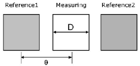
Figure 1: Schematic outline of the reference aperture configurations for two symmetrically placed circular apertures (Gautier et al. 1992).

Measuring the brightness of sources involves subtracting the sky background derived from the well-defined reference. The fluctuations in the surface brightness of extended structure on similar scales to the resolution of the telescope and instrument beam can produce spurious events that can be easily mistaken for genuine point sources. This is because the source detection is usually simply accomplished from the difference in signal between the on-source position and some background position. Therefore sky confusion noise due to the sky brightness fluctuations, $N(\theta)$, is defined as (HB90; Gautier et al. 1992):

$$N(\theta)=\Omega\sqrt{S(\theta)},$$ (1)

where $\Omega$ is the solid angle of the measuring aperture, $\theta$ is the angular separation between the target and reference sky positions, and $S(\theta)$ is the second order structure function, which is defined as [Gautier et al. 1992]:

$$S(\theta)=\left\langle\left|I(x)-\frac{I(x-\theta)+I(x+\theta)}{2}\right|^{2}\right\rangle_{x},$$ (2)

where $I$ is the sky brightness, $x$ is the location of the target, and $\langle~{}\rangle$ represents the average taken over the whole map. For the configuration of two symmetrically placed reference apertures, see Fig. 1.

Although the zodiacal emission is main background source in the short wavelength of far-IR range in low ecliptic latitude regions, it will not contribute to the fluctuations on the large scales because the zodiacal light is generally smooth on scales smaller than typical resolution of IR observations [Reach et al. 1995, Kelsall et al. 1998]. From the analysis of the ISO data, $\acute{\rm A}$brah$\acute{\rm a}$m et al. [$\acute{\rm A}$brah$\acute{\rm a}$m et al. 1997] searched for the brightness fluctuations in the zodiacal light at 25 $\mu$m with 5 fields of $\sim$ 0.5^∘ $\times$ 0.5^∘ at low, intermediate, and high ecliptic latitudes. They found that an upper limit to the fluctuations of 0.2 per cent of the total brightness level was estimated for an aperture of 3^′ diameter. This amount of fluctuations would not cause any significant noise.

Therefore, the sky confusion noise is mainly related to the spatial properties of the cirrus. In many cases, the power spectrum of the dust emission can be expressed as a simple power-law. Using the IRAS data at 100 $\mu$m, Gautier et al. [Gautier et al. 1992] computed the power spectrum $P$ of the spatial fluctuations of cirrus emission as a function of spatial frequency $k$, for angles between 4^′ and 400^′.

$$P=P_{0}\left(\frac{k}{k_{0}}\right)^{\alpha}=P_{0}\left(\frac{d_{0}}{d}\right)^{\alpha},$$ (3)

where $d$ represents the angular scale corresponding angular frequency ($k=\frac{2\pi}{d}$). The subscript 0 on $k$ and $d$ denotes a reference scale, $P_{0}$ is the powers at $k=k_{0}$, and $\alpha$ is the index of the power spectrum. Since the second order structure function is proportional to power spectrum representing the spatial structure of cirrus, the sky confusion noise $N$ on a scale $d$ corresponding to the width of the measurement aperture scales as:

$$N\propto\left(\frac{d}{d_{0}}\right)^{1-\frac{\alpha}{2}}\cdot P_{0}^{\frac{1}{2}}.$$ (4)

HB90 extended the work by Gautier et al. [Gautier et al. 1992] at $\lambda=100~{}\mu$m in order to estimate the sky confusion at all wavelengths, using the empirical relationship, $P_{0}\propto\langle I_{0}\rangle^{3}$ and $\alpha=-3$ in Gautier et al. [Gautier et al. 1992]. They found an approximation for the cirrus confusion noise as follows (hereafter HB90 formula):

$$N=\zeta\left(\frac{\lambda}{100~{}\mu\rm m}\right)^{2.5}\left(\frac{D_{t}}{1~{}\rm m}\right)^{-2.5}\left(\frac{\langle I_{\lambda}\rangle}{1~{}\rm MJy\,sr^{-1}}\right)^{1.5}{\rm mJy},$$ (5)

where $\zeta$ is a constant, $\lambda$ the wavelength of the measurement, $D_{t}$ the diameter of the telescope, and $\langle I_{\lambda}\rangle$ is the mean brightness at the observation wavelength. They set the constant $\zeta$ to be 0.3.

This indicates that the sky confusion depends upon both the variation of the surface brightness in the background structure and the resolution of the telescope. Consequently, the noise becomes less significant for larger aperture sizes.

3 GENERATION OF CIRRUS MAP

In order to investigate the sky confusion for the present and upcoming infrared space missions with a high resolution, we need the information on the behavior of cirrus emission in very small scales. Since observationally available data have rather low resolution, we need to add high resolution component. In this section, we describe the method of extending the low resolution data to high resolution. For the observational low resolution data, we used the all-sky 100 $\mu$m dust map generated from the IRAS and COBE data by Schlegel, Finkbeiner, and Davis (1998; hereafter SFD98).

3.1 Fluctuations at Higher Spatial Resolution

3.1.1 Measured Power Spectrum

Figure 2: Measured power spectrum of dust emission in the dust map by SFD98 (Schlegel, Finkbeiner & Davis 1998). The four curves represent four patches selected in the Northern and the Southern Galactic sky at $b=|50|^{\circ}$.

Fig. 2 shows the measured power spectrum in the dust maps of SFD98 at a Galactic latitude of $b=|50|$ degrees. These power spectra are well fitted to power laws of index -2.9. However, the power drops at higher frequencies corresponding to the map resolution of $\sim$ 6.1 arcmin. This breakdown of the power spectrum is due to the large beam size of IRAS map. Although we can recover the small-scale fluctuation by the deconvolution of a point spread function (PSF), there is clearly some limitation. We need to generate the dust map including the contributions from small-scale fluctuations in order to study for the planned present and future missions with high resolution ($<$ 1 arcmin). We obtain such high resolution map by adding small-scale structure of cirrus emission to the low-resolution map of SFD98 assuming that the small-scale fluctuations also follow the estimated power spectrum with the same power-law index, as described above.

3.1.2 Small Scale of Fluctuations

The power, $P(k)$, is defined as the variance of the amplitude in the fluctuations:

$$P(k)\equiv\langle\mid\delta_{k}\mid^{2}\rangle=\frac{1}{V}\int\xi(x)\frac{\sin(kx)}{kx}4\pi x^{2}dx,$$ (6)

where $\delta_{k}$ is the perturbation field, $\langle\mid\delta_{k}\mid^{2}\rangle$ is the variance of the fluctuation and $\xi(x)$ is the correlation function of the brightness field. We assume that the distribution of fluctuations is approximated as a random Gaussian process where the Fourier components $\delta_{k}$ have random phases so that the statistical properties of distribution are fully described by the power spectrum $\mid\delta_{k}\mid^{2}$ [Peebles 1980]. In this case, we can set each fluctuation within a finite grid in the frequency domain by a random Gaussian process of the amplitude of each fluctuation considering the realization of a volume for the sample embedded within a larger finite volume [Gott et al. 1990, Park et al. 1994, Peacock 1999]. We assign Fourier amplitudes randomly within the above distribution in the finite volume and assign phases randomly between 0 and 2$\pi$. Since the field used in this simulation is small ($<$ 10 degree), we can take the small-angle approximation and treat the patch of sky as flat [White et al. 1999]. In the flat sky approximation, we obtain the power spectrum and generate a patch of the dust map in cartesian coordinates.

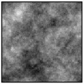
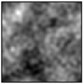
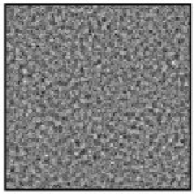
Figure 3: Simulated dust emission map (upper) and the profile of map (lower). The upper-left panel shows the simulated image assuming a power spectrum with a power index of -3. The upper-middle panel and the upper-right panel show only large-scale fluctuations and small-scale fluctuations, respectively. The lower panel shows the one-dimensional profile for a selected part of the upper-left and the upper-middle panel.

We generate a realistic distribution of the Galactic emission in the following manner. The basic data for the information of the large-scale structure are obtained from the low resolution all-sky map by SFD98. We add the simulated small-scale structure to these basic data in the Fourier domain, where the power spectrum of the small-scale structure follows that of the large-scale structure. Fig. 3 shows our simulated emission map including small-scale fluctuations. The left panel of Fig. 3 shows the simulated dust emission image corresponding to a power spectrum with $\alpha=-3$. The middle panel includes only the emission above the resolution of the dust map by SFD98, $\sim$ 6.1 arcmin, (large-scale emission) while the right panel shows the emission above the resolution of the dust map by SFD98 (separated in Fourier domain, i.e., small-scale emission). The lower panel shows the profiles for selected areas of two images (upper-left and upper-middle panels). We find in this simulation that the emission including the high resolution, small-scale component (above the resolution of the dust map by SFD98 to a resolution of 4 arcsec) reflects the trend of the large-scale emission (above the resolution of SFD98 dust map).

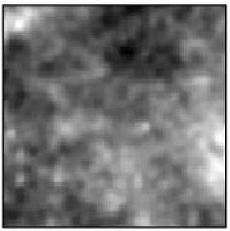
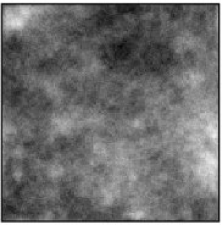
Figure 4: Patch of SFD98 dust map, regenerated patch (upper panel) and the estimated power spectrum (lower panel). The upper-left panel is a patch of the SFD98 dust map at the Galactic latitude of 50 degree and the upper-right panel is the regenerated patch based upon the patch from the SFD98 dust map. The dashed and solid lines in the lower panel show the estimated power spectrum of the upper-left and the upper-right panels, respectively. Note that the Nyquist frequency in the power spectrum of the upper-right panel is 7.5 arcmin^-1, but we only plot to $\sim$ 0.5 arcmin^-1. The dotted line shows the fit to the power spectrum below the spatial cutoff frequency.

We obtain a patch of the dust map including small-scale fluctuations by summing the large-scale component of SFD98 map and the small-scale component of the simulated emission in the Fourier domain. According to this scheme of Fourier power spectrum analysis, the cutoff spatial frequency of the dust map by SFD98 is set to the Nyquist limit, i.e. a half of the spatial frequency corresponding to the resolution of the dust map by SFD98. We use the power spectrum fitted below the Nyquist sampling limit in order to extend the power spectrum to higher spatial frequencies. Typically, the 2D power spectrum of a SFD98 dust map patch shows the presence of a cross along spatial frequencies of $x$ and $y$ axis if we assume that the centre in the spatial domain is regarded as the spatial frequency 0. This cross is caused by the Fast Fourier Transform (FFT) algorithm that makes an “infinite pavement” with the image prior to computing the Fourier transform [Miville-Deschênes et al. 2002]. In order to preserve the information of the emission at the edges, we directly use the power at the spatial frequencies of $x$ and $y$ axis, and extrapolate the power at other spatial frequencies (above the cutoff spatial frequency) according to the estimated power spectrum. In Fig. 4, we show a patch of the dust map by SFD98 at a Galactic latitude of 50 degree (upper left), a patch regenerated by extending the power spectrum (upper right) and the estimated power spectrum (lower panel).

3.2 Dust Emission at Other Wavelengths

Assuming that the spatial structure of the dust emission is independent of wavelength, we can obtain the dust map at other wavelengths than 100 $\mu$m by applying an appropriate model for the Spectral Energy Distribution (SED). Since the dust particles are small ($<$ 0.25 $\mu$m) compared with far-IR wavelengths, the opacity does not depend upon the details of the particle size distribution, but on the nature of the emitting material itself. In the far-IR, the opacity $\kappa_{\nu}$ generally follows a power law:

$$\kappa_{\nu}\propto\nu^{\beta}$$ (7)

with frequency $\nu$.

The SED may be approximated as one-component or two-component models [Schlegel, Finkbeiner & Davis 1998, Finkbeiner et al. 1999]. The dust temperature map is constructed from the COBE Diffuse Infrared Background Experiment (DIRBE) 100 $\mu$m and 240 $\mu$m data [Boggess et al. 1992] which was designed to search for the cosmic IR background radiation. For a one-component moedel, the emission $I_{\nu}$ at frequency $\nu$ can be expressed as

$$I_{\nu}=K_{100}^{-1}(\beta,T)\,I_{100}\,\frac{\nu^{\beta}B_{\nu}(T)}{\nu_{0}^{\beta}B_{\nu_{0}}(T)},$$ (8)

where $B_{\nu}(T)$ is the Planck function at temperature $T$, $I_{100}$ is the DIRBE-calibrated 100 $\mu$m map, $K_{100}^{-1}(\beta,T)$ is the colour correction factor for the DIRBE 100 $\mu$m filter when observing a $\nu^{\beta}B_{\nu}(T)$ spectrum (DIRBE Explanatory Supplement 1995). Although the generated temperature maps have relatively low resolution (1.3^∘) compared with our simulated dust map patch, we interpolate this map to small grid sizes ($<$ 10 arcsec). Taking the emissivity model with $\beta=2$ [Draine & Lee 1984], we can obtain the dust temperature from the DIRBE 100 $\mu$m/240 $\mu$m emission ratio.

Figure 5: Comparison between the one-component dust model and the two-component dust model for one small patch. The dust emission of the two-component model in the wavelength range from 120 $\mu$m to 200 $\mu$m is slightly higher than that of the one-component model due to the dominant contribution by carbon grains.

Based upon laboratory measurements, a multicomponent model for interstellar dust has been constructed by Pollack et al. [Pollack et al. 1994]. In order to solve the inconsistency of the $\nu^{2}$ emissivity model in the 100 $-$ 2100 GHz (3000 $-$ 143 $\mu$m) emission, Finkbeiner et al. [Finkbeiner et al. 1999] used a two-component model where diverse grain species dominate the emission at different frequencies in order to fit the data of the COBE Far Infrared Absolute Spectrophotometer (FIRAS). Assuming that each component of the dust has a power-law emissivity over the FIRAS range, Finkbeiner et al. [Finkbeiner et al. 1999] constructed the emission $I_{\nu}$ in multicomponent model:

$$I_{\nu}=\frac{\sum_{i}~{}f_{i}~{}Q_{i}(\nu)~{}B_{\nu}(T_{i})}{\sum_{i}~{}f_{i}~{}Q_{i}(\nu_{0})~{}B_{\nu_{0}}(T_{i})~{}K_{100}(\beta_{i},T_{i})}\,I_{100},$$ (9)

where $f_{i}$ is a normalization factor for the $i$-th grain component, $T_{i}$ is the temperature of component $i$, $K_{100}$ is the DIRBE colour-correction factor and $I_{100}$ is the SFD98 100 $\mu$m flux in the DIRBE filter. The emission efficiency $Q_{i}(\nu)$ is the ratio of the emission cross section to the geometrical cross section of the grain component $i$. In order to obtain the temperature of each component, we further need effective absorption opacity defined by

$$\kappa_{i}^{*}={\int_{0}^{\infty}\kappa_{i}^{\rm abs}J_{\rm ISRF}(\nu)d\nu\over\int_{0}^{\infty}J_{\rm ISRF}(\nu)d\nu},$$ (10)

where $\kappa_{i}^{\rm abs}$ is the absorption opacity of the $i$-th component, and $J_{\rm ISRF}$ is the mean intensity of interstellar radiation field. Finkbeiner et al. [Finkbeiner et al. 1999] assumed that the normalization factors do not vary with locations and size independent optical properties of dust grains. The emission efficiency factor $Q_{i}$ at far-IR is further assumed to follow a power-law with different indices ($\beta$) for different dust species. In the present work, we adopted the ‘best-fitting’ two-component model by Finkbeiner et al. [Finkbeiner et al. 1999]: $\beta_{1}=1.67$, $\beta_{2}$=2.70, $f_{1}=0.0363$, $f_{2}=0.9637$, and $q_{1}/q_{2}=13.0$, where $q_{i}=\kappa_{i}^{\rm abs}(\nu_{0})/\kappa_{i}^{*}$ which represents the ratio of far-IR emission cross section to the UV/optical absorption cross section. The reference frequency $\nu_{0}$ is that corresponding to wavelength 100 $\mu$m.

If we further assume that the interstellar radiation field has constant spectrum, the temperature of each component can be uniquely determined by the far-IR spectrum represented by the DIRBE 100 $\mu$m/240 $\mu$m ratio. A two-component model provides a fit to an accuracy of $\sim$ 15 per cent to all the FIRAS data over the entire high-latitude sky. In Fig. 5, we see the dust emission for the one-component and two-component dust models [see Schlegel et al. [Schlegel, Finkbeiner & Davis 1998]; Finkbeiner et al. [Finkbeiner et al. 1999]]. The two-component model agrees better with the FIRAS data in the wavelength range longer than 100 $\mu$m where the dust emission estimated from one-component model is significantly lower than the estimate from the two-component model.

In two models, the contribution of the small grains resulting in an excess below 100 $\mu$m is not considered. Since there is no significant difference between models below 100 $\mu$m while the dust emission of the two-component model is slightly higher than that of the one-component model in wavelengths ranging from 120 to 200 $\mu$m, we use the two-component model in our calculations.

Through a PSF convolution at each wavelength and a wavelength integration over a 5 $\mu$m wavelength grid, we obtain the high resolution dust map in other bands.

4 FLUCTUATION ANALYSIS FOR SKY CONFUSION NOISE

Among the parameters affecting the sky confusion noise, most of them depend upon the mean brightness, the spatial structure of the cirrus, and the observing wavelength, as seen in equation (5). In Table 1, we list the basic instrumental parameters of present and future IR space missions; the aperture of the telescope, Full Width at Half Maximum (FWHM) of the beam profile and the pixel size for each detector. For comparison with previous studies [Herbstmeier et al. 1998, Kiss et al. 2001], we include the specifications for ISO. We select a short wavelength band (SW) and a long wavelength band (LW) for each mission.

Table 1: Instrumental parameters for various space missions.

	Aperture	Wavelength		FWHM a		Pixel size
	(meter)	($\mu$m)		(arcsec)		(arcsec)
Space Mission		SW	LW	SW	LW	SW	LW
ISO b	0.6	90	170	31.8	60	46	92
Spitzer c	0.85	70	160	16.7	35.2	9.84	16
ASTRO-F d	0.67	75	140	23	44	26.8	44.2
Herschel e	3.5	70	160	4.3	9.7	3.2	6.4
SPICA	3.5	70	160	4.3	9.7	1.8	3.6

^a FWHM of diffraction pattern.

^b Two ISOPHOT filters (C1_90 in SW band and C2_170 in LW band).

^c MIPS bands for the Spitzer mission.

^d ASTRO-F/FIS (Far Infrared Surveyor) has a WIDE-S band in SW and WIDE-L band in LW.

^e PACS have ‘blue’ array in short wavelength (60-85$\mu$m or 85-130$\mu$m) and the ‘red’ array in long wavelength (130-210$\mu$m).

In order to examine the dependency of the sky confusion noise on the instrumental parameters, we list sky confusion $N$ estimated from HB90 formula for each mission considered in this work in Table 2. As the aperture of the telescope becomes larger or the wavelength becomes shorter, sky confusion $N$ should become correspondingly smaller. In Section 3, we obtained the dust maps extended to high spatial resolution over a wide spectral range. With this simulated dust map, we estimate the sky confusion noise for various space mission projects.

Table 2: Sky confusion noise estimated from HB90 formula for each space mission. The instrumental parameters for each mission are given in Table 1. The mean brightness here is fixed to be 1 MJy sr^-1.

	$N$ (mJy)
Space Mission	SW	LW
ISO	0.83	4.05
Spitzer	0.18	1.46
ASTRO-F	0.40	1.89
Herschel	0.0054	0.042
SPICA	0.0054	0.042

4.1 Selected Regions

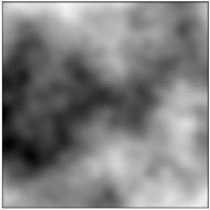
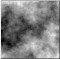
Figure 6: PSF-convolved patch of the dust map for space mission; ISO (upper-left), ASTRO-F (upper-right), Spitzer (lower-left), Herschel/SPICA (lower-right) missions.

Table 3: Properties of the selected regions. The Galactic longitude of all patches is 0^∘. I₀ is a mean sky brightness, $\alpha$ is the power index of the power spectrum, and P₀ is the power estimated at 0.01 arcmin^-1 and 100 $\mu$m.

	I0 a			$\alpha$ b	$\log$ P0 c
	(MJy sr-1)				(Jy2 sr-1)
Region a	70$\mu$m	100$\mu$m	160$\mu$m
$b$=10∘	5.4	24.4	53.9	-3.45$\pm$0.11	9.00$\pm$0.17
$b$=17∘	3.5	18.6	45.3	-3.50$\pm$0.16	9.05$\pm$0.24
$b$=22∘	3.5	15.3	34.1	-3.54$\pm$0.15	8.48$\pm$0.22
$b$=28∘	2.2	8.9	24.7	-3.50$\pm$0.15	7.74$\pm$0.21
$b$=36∘	1.2	6.0	14.4	-3.80$\pm$0.10	7.41$\pm$0.15
$b$=45∘	0.6	2.8	6.2	-3.13$\pm$0.12	6.39$\pm$0.18
$b$=59∘	0.3	1.4	2.9	-2.99$\pm$0.09	6.00$\pm$0.13
$b$=70∘	0.2	1.2	2.6	-3.20$\pm$0.10	6.27$\pm$0.15
$b$=84∘	0.1	0.8	1.8	-2.87$\pm$0.09	5.77$\pm$0.14
$b$=90∘	0.1	0.5	1.4	-2.87$\pm$0.08	5.66$\pm$0.12

We generate the PSF-convolved patches of a dust map as a function of increasing Galactic latitude (decreasing sky brightness) from 0.3 MJy sr^-1 to 25 MJy sr^-1 at 100 $\mu$m at a resolution of 1 arcsec by using the method explained in Section 3. The size of the simulated image is 1.3^∘ $\times$ 1.3^∘. For the PSF, we used an ideal circular aperture Airy pattern corresponding to the aperture size of telescopes. In Fig. 6, we can see the PSF-convolved small patch of dust map (900$\arcsec$ $\times$ 900$\arcsec$) for each space mission. As the aperture of the telescope becomes larger, the structures that can be visible become smaller. Since the cirrus emission generally depends upon the Galactic latitude, we select the patches as a function of the Galactic latitude. We list the properties of selected regions at a Galactic longitude of 0^∘ among 50 patches in Table 3. The estimated power spectrum in Table 3 differs from patch to patch. In order to reflect the large structure of the dust map and reduce the discrepancies of the power spectrum between adjacent patches, we use a large area around the patch ($\sim$ 2.5^∘ $\times$ 2.5^∘) in the measurement of the power spectrum.

4.2 Estimation of Sky Confusion Noise

4.2.1 Contribution of Instrumental Noise

In order to estimate the sky confusion noise, the structure function for the cirrus emission patch obtained by measuring the sky brightness fluctuations is widely used [Gautier et al. 1992, Herbstmeier et al. 1998, Kiss et al. 2001]. The size of the measuring aperture is set to be the FWHM of each beam profile if the detector pixel size is smaller than the FWHM of a beam profile. Since the sky confusion noise and the instrumental noise are statistically independent [Herbstmeier et al. 1998, Kiss et al. 2001], the measured noise $N_{\rm meas}$ is

$$N_{\rm meas}^{2}=N^{2}+\eta\cdot\sigma_{\rm inst}^{2},$$ (11)

where $N$ is the sky confusion noise corresponding 1$\sigma$, $\sigma_{\rm inst}$ is the instrumental noise, and $\eta$ is the contribution factor from the instrumental noise. The contribution factor $\eta$ can be determined by the size of the measurement aperture and the separation (see equation 2 and Fig. 1).

4.2.2 Comparison with Other Results

We estimate the sky confusion noise from the patches of the simulated sky map. In Fig. 7, we plot the fractional area as a function of sky brightness over the whole sky to visualize the sky brightness distribution.

Figure 7: The fraction of the sky brightness for all sky. Note that most of the sky have the sky brightness below 1 MJy sr^-1 (SW) and 15 MJy sr^-1 (LW). The contribution in the highest mean brightness resulted from near the Galactic center.

Since we consider the sky confusion caused solely by the emission from cirrus structures, we do not include any contribution from the instrumental noise.

In order to determine a dependency of the sky confusion noise on separation, we performed a “calculation” for the estimation of sky confusion noise for given mean brightness of the sky patch for each space mission (ISO, Spitzer, ASTRO-F, and Herschel/SPICA) by systematically varying the value of $s$ from 2 to 7, using equation (2), where $s$ parameter is related to the separation $\theta$ = $sD$. Generally, larger separation causes larger sky confusion noise because we may be estimating the fluctuations from different structures. In practical photometry, large separations are generally used, i.e., $\theta$ = $sD$, $s>2$ in the configuration of Fig. 1 [Kiss et al. 2001, Laureijs et al. 2003]. As a reference, we take the estimate of the sky confusion noise with $s=2.5$ for a comparison of the measured sky confusion with the photometric results given in Section 5. In the source detection, the background estimation parameter have the same role with the separation parameter. We found the optimal value for the background estimation parameter through the photometry (see Section 5.2 for detailed explanation).

In Figs 8 – 11, we present our estimates of the sky confusion noise for the ISO, Spitzer, ASTRO-F and Herschel/SPICA space missions comparing the formula for the sky confusion noise predicted by HB90 (hereafter HB90 formula). For ISO results, the sky confusion noise with $s=2.5$ is overestimated for the dark fields, but underestimated for the bright fields (see Fig. 8). With larger separations, e.g., $s=7$, the estimated confusion noise approaches the HB90 formula although it is still overestimated for the dark fields. We can see the same tendency in other studies in the sky confusion noise measured from ISO observations [Herbstmeier et al. 1998, Kiss et al. 2001]. The measured sky confusion noise for the Spitzer and Herschel/SPICA missions are much lower than the predictions of HB90 except for the dark fields (see Figs 10 and 11).

Comparing the empirical relation between $P_{0}$ and $I_{0}$ by Gautier et al. [Gautier et al. 1992], we present our estimated $P_{0}$ in Fig. 12. It shows a lower $P_{0}$ in bright fields and the higher $P_{0}$ in dark fields could cause an underestimation in the bright fields and an overestimation in the dark fields of the sky confusion noise. Such inconsistencies, overestimation of $P_{0}$ in bright fields and underestimation of $P_{0}$ in dark fields, also appear in other regions of the sky. By fitting our estimations of $P_{0}$, we obtained a new relation between the $P_{0}$ and $I_{0}$. The HB90 formula assumed the wavelength dependency only through the beam size. However, although the cirrus structure is generally preserved in other wavelengths, the empirical relation should be scaled according to the variation of the cirrus brightness with wavelength, i.e, cirrus spectral energy distribution. Therefore, in order to apply our empirical formula to other wavelength bands, we need some additional correction. For this correction, we used the ratio of the mean brightness at the two wavelengths, e.g., $I_{160\mu\rm m}$/$I_{100\mu\rm m}$ $\sim$ 2 (see Table 3). For comparison with the sky confusion noise estimated from the ISO mission, we plot the HB90 formula to which our empirical relation is applied (see thick dotted line in Fig. 8). Although our formula solve the discrepancies of our estimations to some extent, there are still disagreements especially with the results for higher resolution missions.

The HB90 formula was obtained from the analysis of the low resolution IRAS data at 100 $\mu$m and assumed a constant power index for the cirrus power spectrum. In the case of the high resolution missions, since the sky confusion becomes sensitive to the local structure rather than the large scale structure, the calculation of the sky confusion strongly depends upon the power spectrum estimated for each patch and the power at the scale length corresponding to the resolution of the detector. Therefore, we should consider carefully the combination of the resolution and the power spectrum of the cirrus in the estimation of the sky confusion noise. In addition, the larger discrepancy in the bright regions for the ASTRO-F mission compared to the prediction from ISO observations can be explained by an increase in the spatial resolution, although the aperture sizes of two telescopes are similar (see the specifications of the two space missions in Table 1). We conclude that the sky confusion level predicted by the IRAS data from which HB90 formula are derived is significantly overestimated in the case of the higher resolution missions.

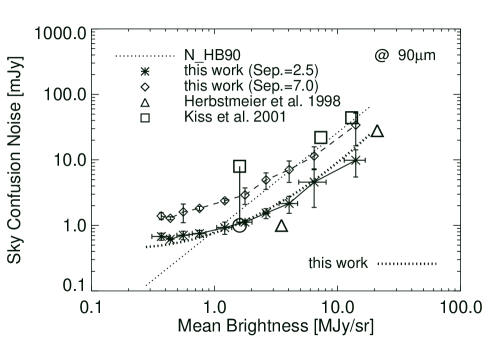
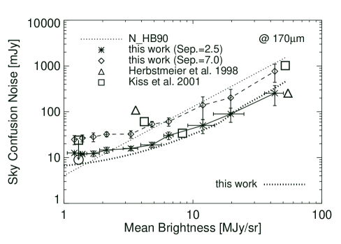
Figure 8: Estimated sky confusion noise for the ISO mission. Upper and lower panels show the sky confusion noise at 90 $\mu$m and 170 $\mu$m, respectively. The dotted line shows the sky confusion noise by HB90 (Helou & Beichman 1990). The symbols are the estimated sky confusion noise on averaging 5 patches with similar mean brightness. For comparison, we plot the estimated sky confusion noise for the larger separation of $s=7$. The circle symbol means the sky confusion noise correcting the contribution from the CFIRB. The thick dotted line is the HB90 formula to which our empirical relation is applied.

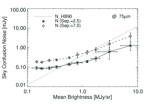
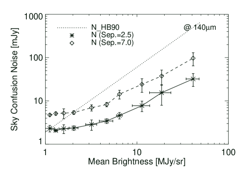
Figure 9: Estimated sky confusion noise for the ASTRO-F mission. Left and right panels show the sky confusion noise in the WIDE-S band (75 $\mu$m) and WIDE-L band (140 $\mu$m), respectively. The symbols and lines are same as given in Fig. 8.

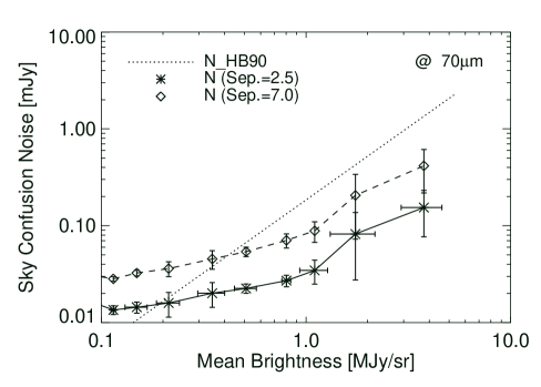
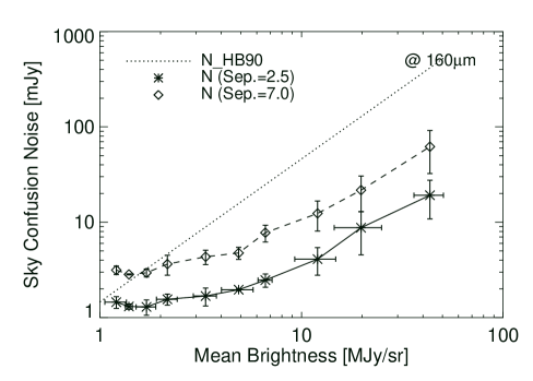
Figure 10: Estimated sky confusion noise for the Spitzer mission. Left and right panels show the sky confusion noise for the MIPS 70 $\mu$m and 160 $\mu$m bands, respectively. The symbols and lines are same as in Fig. 8.

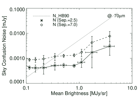
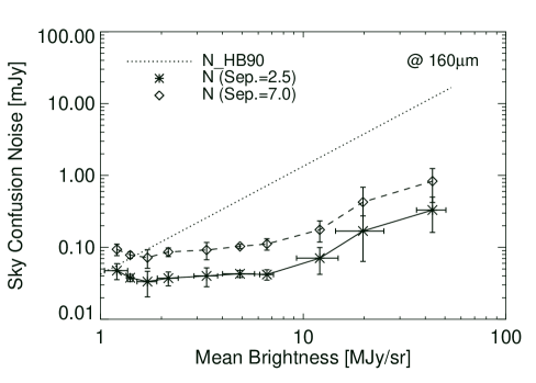
Figure 11: Estimated sky confusion noise for the Herschel and SPICA missions. Left and right panels show the sky confusion noise at 70 $\mu$m and 160 $\mu$m, respectively. The symbols and lines are same as in Fig. 8.

Figure 12: The relation between $P_{0}$ and $B_{0}^{3}$. The dotted line is the result from Gautier et al. (1992), the symbol is from our estimated $P_{0}$, and the dashed line is the fit to our result. In bright fields, values of $P_{0}$ expected from Gautier et al. (1992) have higher values than those measured from our patches in bright fields.

Generally the most important component superimposed on the extragalactic background in the far-IR is the cirrus emission. However, at high spatial frequencies the Cosmic Far-IR Background (CFIRB) fluctuations may become dominant [Schlegel, Finkbeiner & Davis 1998, Guiderdoni et al. 1997, Juvela, Mattila & Lemke 2000]. Therefore, in any estimation of the sky confusion noise using observational data in the dark fields should consider the fluctuation due to the CFIRB. By fitting the sky confusion noise over the mean sky brightness, Kiss et al. [Kiss et al. 2001] obtained CFIRB fluctuation of 7 $\pm$ 2 mJy at 90 $\mu$m and 15 $\pm$ 4 mJy at 170 $\mu$m. After correcting for the contribution of the CFIRB in the estimation of the sky confusion noise, we obtained results similar with those of Kiss et al. [Kiss et al. 2001] in the dark fields (see the symbol in circle with arrow in Fig. 8 at the mean brightness of $\sim$ 1.5 MJy/sr). Since the CFIRB fluctuations strongly depend upon the extragalactic source count model, we will discuss this issue in greater detail in our forthcoming paper [Jeong et al. 2004c [Jeong et al. 2004c, in preparationPaper II], in preparation].

4.2.3 Sky Confusion Noise for Various Separations

Kiss et al. [Kiss et al. 2001] analyzed the dependency of the sky confusion noise on other separations by the simple power expression from ISO observational data:

$$N(q\theta_{\rm min})=N(\theta_{\rm min})\times q^{\gamma},$$ (12)

where $q>1$ and $\gamma$ is a constant for a specific map. We obtained $\gamma$’s for all patches and showed $\gamma$ as a function of mean brightness for each mission as given in Fig. 13. As the sky becomes brighter, $\gamma$ becomes larger due to the prominent structure of the cirrus emission. Kiss et al. [Kiss et al. 2001] obtained a much lower $\gamma$ in dark regions, but their values of $\gamma$ in other regions are similar to our results. This result can be explained by two possible effects: one is that the cirrus structure observed by ISO is blurred by the instrumental noise in most of the dark regions and the other is that many extragalactic point sources below the detection limit, i.e. CFIRB fluctuations, can remove the cirrus structure. If we only consider the component due to the cirrus in the dark fields, the values of $\gamma$ in the dark regions by Kiss et al. [Kiss et al. 2001] are similar to our results. In most of the bright regions, the scatter of $\gamma$ shows the similar trend and this is probably caused by the relatively large difference in the spatial structure in each region. In the same mean brightness, $\gamma$’s in SW band are larger than those in LW band because spatial structures should be prominent in SW band. In addition, since we use the simulated data, changing features of $\gamma$ in two wavelength have a similar shape. For the Herschel and SPICA missions, our estimations show that $\gamma$ slowly increases and the error decreases compared with other missions, because of the much higher resolution than the other missions considered.

Figure 13: Dependency of the sky confusion noise on separation for ISO, ASTRO-F, Spitzer, Herschel and SPICA, respectively. The dotted line and the dashed line is a fit to our estimation analysis data for SW and LW band, respectively. In the brighter regions, $\gamma$ has higher values than in the dark fields.

4.2.4 Effect of Power Index $\alpha$

In this study, we assume that the structure of cirrus is independent of wavelength. However, recent papers reported on enhanced dust emissivity at some medium-to-high density clouds in LW band of Far-IR due to the presence of a cold dust component (T $\leq$ 15K) [Cambr$\acute{\rm e}$sy et al. 2001, del Burgo et al. 2003, Stepnik et al. 2003]. This result imply that the cirrus structure can be changed in LW band. Kiss et al. [Kiss et al. 2003] suggested that the power index of the power spectrum also depends upon both wavelength and surface brightness due to the coexistence of dust components with various temperatures within the same field and cold extended emission features (usually, $-2.0<\alpha<-4.0$). Using the assumption that the sky confusion noise is proportional to the scale length (see equation 4), we can estimate the sky confusion for different power indices. The ratio $\psi$ of the sky confusion noise with the power index of $\alpha+\epsilon$ to that with the power index of $\alpha$ can be defined as

$$\psi=\frac{N(\alpha+\epsilon)}{N(\alpha)},$$ (13)

where $\epsilon$ is the contribution to the power index from any other structure in the power spectrum. In this calculation, we fix the power at the scale length of the resolution limit of the map ($\sim$ 6.1 arcmin) and wavelength at 100 $\mu$m from the assumption that the power over this scale is not affected by the extra components proposed by Kiss et al. [Kiss et al. 2003]. Table 4 lists the ratio of the sky confusion noise for the different power indices for each space mission covering power indices of the power spectrum on the cirrus emission. Since the fluctuation at smaller scales is more sensitive to the power index, the sky confusion noise is much more dependent upon the power index for the space missions with higher resolutions. As seen in Table 3, our estimated power indices in the bright regions ($\alpha$ $>$ 3.3) are somewhat higher than those in low density regions ($\alpha$ $<$ 2.8). From the recent Spitzer observation, Ingalls et al. [Ingalls et al. 2004] obtained the power index of -3.5 at 70 $\mu$m in the Gum Nebula. Therefore, if this varying power index is not so large, it does not affect severely the final sensitivity values.

Table 4: Ratio $\psi$ of the sky confusion noise for the different power indices.

	$\epsilon$ a = -1.0		$\epsilon$ = 1.0
Space Mission	SW	LW	SW	LW
ISO	0.13	0.19	1.7	1.2
Spitzer	0.083	0.12	2.8	1.9
ASTRO-F	0.10	0.13	2.2	1.8
Herschel	0.041	0.061	5.6	3.8
SPICA	0.041	0.061	5.6	3.8

^a contribution index in the power spectrum.

5 PHOTOMETRIC MEASUREMENTS OF SKY CONFUSION NOISE

In Section 4, we estimated the sky confusion noise by the fluctuation analysis. The sky confusion noise should affect the source detection efficiency, causing a deterioration in the detection limit. In this section, we obtain the measured sky confusion noise by carrying out photometry on realistically simulated data.

5.1 Source Distribution

The distribution of sources per unit area on the sky can be described as a function of the flux density and depends upon both the spatial distribution of the sources and their luminosity function. For simplicity, we assume the number of sources whose flux is greater than flux $F$, $n(>F)$, is a power-law function of $F$,

$$n(>F)=n_{0}(>F_{0})\left({F\over F_{0}}\right)^{-\omega},$$ (14)

for $F_{\rm min}<F<F_{\rm max}$, where $n_{0}$ and $F_{0}$ are normalization constants for number of sources and for flux, respectively, $F_{\rm min}$ is the minimum flux, $F_{\rm max}$ is the maximum flux in the source distribution.

The source confusion caused by the overlapping of adjacent sources mainly depends upon the source distribution and the beam profile [Condon 1974, Franceschini et al. 1989]. Source confusion becomes important as the observation sensitivity increases since there are usually more faint sources than brighter ones. Currently favorable source count models require strong evolution in order to fit the ISO data from mid- to far-IR, the SCUBA data at sub-mm wavelengths, and the Cosmic Infrared Background (CIRB) at 170 $\mu$m [Oliver et al. 1997, Smail, Ivison & Blain 1997, Kawara et al. 1998, Hughes et al. 1998, Aussel et al. 1999, Puget et al. 1999, Efstathiou et al. 2000, Serjeant et al. 2000, Lagache et al. 2000, Matsuhara et al. 2000, Scott et al. 2002]. In our study, we use a simple source distribution for the purpose of investigating only the effect of the sky confusion. We will discuss the source confusion with more realistic source count models in the forthcoming paper. In order to avoid the contributions from any source confusion itself, we assume rather sparse distribution of sources. However, the estimate of detection limit becomes rather uncertain, if there are too few sources. Therefore, we have employed a model for the $n(F)$ utilizing a distribution with two slopes, $\omega$ = 1.0 for bright flux region and $\omega$ = 0.3 for faint flux region (see Fig. 14), in order to derive an accurate value for the sky confusion limits without source confusion effect. Since the sky confusion noises in the SW bands are much lower than those in the LW bands, we set different normalization constants and minimum flux values $F_{\rm min}$, i.e., $F_{\rm min}$ = 0.001 mJy and $n_{0}(>F_{0})$ = 3 in the SW band, $S_{\rm min}$ = 0.1 mJy and $n_{0}(>F_{0})$ = 10 in the LW band, where $F_{0}$ is set to be 100 mJy (see Fig. 14).

Figure 14: Source distribution in the SW band and LW band. We use different slopes ($\omega$ = 1.0 and $\omega$ = 0.3) for the power law source distribution at the boundary flux of 10 mJy in order to reduce the effect of the source confusion.

5.2 Source Detection

We generate images including point sources convolved with the beam profile of each mission using the source distribution described in Section 5.1. Fig. 15 shows the simulated images for the various missions considered. As the detector pixel and the beam profile become smaller, more sources and smaller structure in the cirrus emission appear.

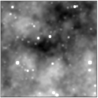
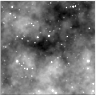
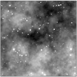
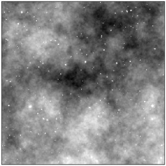
Figure 15: Simulated images including point sources in the LW band for ISO (upper-left), ASTRO-F (upper-right), Spitzer (lower-left), Herschel and SPICA (lower-right) missions. The mean brightness of the cirrus background is 2 MJy sr^-1 at 160 $\mu$m.

We carried out aperture photometry on the simulated images using the SExtractor software v2.2.2 [Bertin & Arnouts 1996]. There are several parameters to be fixed to perform the photometry, but the most influential parameters are the size of a background mesh for estimating background level and the threshold for the source detection in this aperture photometry. In order to optimise for better reliability of the detected sources and reducing the rate of false detection, we make trials by changing two parameters. Finally, we set the size of the background mesh to be 2.5 times of the measuring aperture, and the detection threshold as 4$\sigma$. The final detection limit is determined by the minimum flux of detected point sources. We found that the detection limits determined from 4$\sigma$ criteria are consistent with the 4 times of sky confusion noise measured from the fluctuation analysis. Note that our sky confusion noise estimated from the fluctuation analysis is a 1$\sigma$ fluctuation. In Fig. 16, we compare the detection limit by photometry with the sky confusion noise for each mission. For the ISO and ASTRO-F missions, the results from photometry give relatively higher detection limits than the theoretical estimations via fluctuation analysis. This trend results from the larger detector pixel size compared to the FWHM of the beam profile. The large detector pixel size of the ISO mission significantly degraded the performance of the detection of the point sources (e.g., the left panels in Fig. 16).

Figure 16: Estimated detection limit by photometry. Figures show the detection limit and 4 times sky confusion noise estimated from the fluctuation analysis for the ISO and ASTRO-F missions (left) and Spitzer, Herschel and SPICA missions (right). Upper and lower panels show the results for the SW band and LW band, respectively.

6 SUMMARY AND DISCUSSION

Based on the observed 100 $\mu$m dust map and the models of a dust spectrum, we generated high resolution background maps at wavelengths ranging from 50 to 200 $\mu$m. Using these simulated cirrus maps, we estimated the sky confusion noise for various IR space missions such as ISO, Spitzer, ASTRO-F, Herschel and SPICA. Since we have the observational results only from ISO, we compared the results of our simulation with the ISO data. We found that the sky confusion noise estimated with our simulated maps are consistent with the ISO results. However, in the dark fields the sky confusion noise is more weakly dependent upon the beam separation parameter than in the bright fields in the case of the ISO observation. We conclude that this is due to the fact that the instrumental noise dominates in the dark regions or alternatively, the CFIRB fluctuation is more important. We also found that the sky confusion predicted from the IRAS data is significantly overestimated in the case of the large aperture telescopes, except for the dark fields.

We have confirmed our results through a realistic simulation. We performed photometry on simulated images including point sources with a sparse source distribution in order to avoid the effects of confusion due to crowded point sources. The detection limits obtained from the photometric analysis agree with the sky confusion noise estimated using fluctuation analysis except for ISO and ASTRO-F. The discrepancies for these missions are due to the large detector pixel size compared to the FWHM of the beam size.

The mean brightness of the cirrus emission usually decreases with increasing Galactic latitude [Boulanger & P$\acute{\rm e}$rault 1988]. In order to estimate the detection limits as a function of Galactic latitude, we derived a simple formula for each wavelength band. Because the cirrus emission is extremely strong near the Galactic centre, we excluded the Galactic latitudes $|b|<10^{\circ}$. Fig. 17 shows the detection limits as a function of Galactic latitude. The detection limits for all missions appear to saturate beyond $b\sim 30^{\circ}$.

Figure 17: Detection limits due to the Galactic cirrus as a function of Galactic latitude. The two line plotted for each mission are for the SW band (lower line) and the LW band (upper line).

Fig. 18 summarises the final detection limits for point sources at mean and low sky brightness regions due to the Galactic cirrus. In addition, we also plot the currently estimated 5$\sigma$ detection limits for sources of each mission. The detection limits only take into account the instrumental noise. The instrumental noise for ASTRO-F mission is explained in detail in Jeong et al. (2003; 2004a; 2004b). The integration time is 500 sec for the Spitzer mission (Spitzer Observer’s Manual) and 1 hour for the Herschel mission [Pilbratt 2003]. As shown in Fig. 18, sky confusion almost approaches the detection limit in the LW band of the ASTRO-F and Spitzer missions. Although the sky confusion does not severely affect the detection limits of Herschel mission, it can affect the detection limit of the SPICA because it will have a large aperture telescope cooled to very low temperatures in order to achieve exceptional sensitivity in the far-IR (see Nakagawa 2004 for the detailed information of the SPICA mission).

Figure 18: Detection limits due to Galactic cirrus at mean and low sky brightness in each band. The mean sky brightness in the SW and LW bands is set to 1 MJy sr^-1 and 15 MJy sr^-1, respectively. The lower value for each detection limit corresponds to the detection limit at low sky brightness usually at high Galactic latitudes. The symbol shows the 5$\sigma$ sensitivity for the ASTRO-F, Spitzer, Herschel missions without confusion and the error bar corresponds to 1$\sigma$ sensitivity.

References

- [brahm et al. 1997] brahm P., Leinert C., Lemke D., 1997, A&A, 328, 702
- [Aussel et al. 1999] Aussel H., Cesarsky C. J., Elbaz D., Starck J. L., 1999, A&A, 342, 313
- [Bertin & Arnouts 1996] Bertin E., Arnouts S., 1996, A&AS, 117, 393
- [Boggess et al. 1992] Boggess N. W. et al., 1992, ApJ, 397, 420
- [Boulanger & Prault 1988] Boulanger F., Prault M., 1988, ApJ, 330, 964
- [Cambrsy et al. 2001] Cambrsy L., Boulanger F., Lagache G., Stepnik B., 2001, A&A, 375, 999
- [Condon 1974] Condon J. J., 1974, ApJ, 188, 279
- [del Burgo et al. 2003] del Burgo C., Laureijs R. J., brahm P., Kiss Cs., 2003, MNRAS, 346, 403
- [Draine & Lee 1984] Draine B. T., Lee H. M., 1984, ApJ, 285, 89
- [Efstathiou et al. 2000] Efstathiou A. et al., 2000, MNRAS, 319, 1169
- [Finkbeiner et al. 1999] Finkbeiner D. P., Davis M., Schlegel D. J., 1999, ApJ, 524, 867
- [Franceschini et al. 1989] Franceschini A., Toffolatti L., Danese L., De Zotti G., 1989, ApJ, 344, 35
- [Gallagher et al. 2003] Gallagher D. B., Irace W. R., Werner M. W., 2003, SPIE, 4850, 17
- [Gautier et al. 1992] Gautier T. N. III, Boulanger F., Prault M., Puget J. L., 1992, AJ, 103, 1313
- [Gott et al. 1990] Gott J. R., Park C., Juszkiewicz R. et al., 1990, ApJ, 352, 1
- [Guiderdoni et al. 1997] Guiderdoni B. et al., 1997, Nature, 390, 257
- [Helou & Beichman 1990] Helou G., Beichman C. A., 1990, Proc. of the 29th Liege International Astrophysical Coll., ESA Publ., 117 (HB90)
- [Herbstmeier et al. 1998] Herbstmeier U., brahm P., Lemke D., Laureijs R. J., Klasss U. et al., 1998, A&A, 332, 739
- [Hughes et al. 1998] Hughes D. et al., 1998, Nature, 394, 241
- [Ingalls et al. 2004] Ingalls J. G. et al., 2004, ApJS, 154, 281
- [Jeong et al. 2003] Jeong W.-S., Pak S., Lee H. M. et al., 2003, PASJ, 55, 717
- [Jeong et al. 2004a] Jeong W.-S., Pak S., Lee H. M. et al., 2004a, Adv. Space Res., 34, 573
- [Jeong et al. 2004b] Jeong W.-S., Pak S., Lee H. M. et al., 2004b, Adv. Space Res., 34, 578
- [Jeong et al. 2004c, in preparationPaper II] Jeong W.-S., C. P. Pearson et al., 2004c, in preparation (Paper II)
- [Juvela, Mattila & Lemke 2000] Juvela M., K. Mattila, D. Lemke, 2000, A&A, 360, 813
- [Kawara et al. 1998] Kawara K. et al., 1998, A&A, 336, L9
- [Kelsall et al. 1998] Kelsall T. et al., 1998, ApJ, 508, 44
- [Kiss et al. 2001] Kiss Cs., brahm P., Klaas U., Juvela M., Lemke D., 2001, A&A, 379, 1161
- [Kiss et al. 2003] Kiss Cs., brahm P., Klaas U. et al., 2003, A&A, 399, 177
- [Lagache et al. 2000] Lagache G., Haffner L. M., Reynolds R. J., Tufte S. L., 2000, A&A, 354, 247
- [Laureijs et al. 2003] Laureijs R. J., Klaas U., Richards P. J. et al., 2003, The ISO Handbook Vol IV: PHT - The Imaging Photo-Polarimeter, Version 2.0.1, ESA-SP 1262, European Space Agency
- [Low et al. 1984] Low F. J., Beintema T. N., Gautier F. C. et al., 1984, ApJ, 278, 19L
- [Matsuhara et al. 2000] Matsuhara H. et al., 2000, A&A, 361, 407
- [Miville-Deschênes et al. 2002] Miville-Deschênes M.-A., Lagache G., Puget J.-L., 2002, A&A, 393, 749
- [Murakami 1998] Murakami H., 1998, SPIE, 3356, 471
- [Nakagawa 2001] Nakagawa T., 2001, in the Proc of The Promise of the Herschel Space Observatory, ed. G. L. Pilbratt, J. Cernicharo, A. M. Heras, T. Prusti, & R. Harris, ESA-SP, 460, pp. 67-74
- [Nakagawa 2004] Nakagawa T., 2004, Adv. Space Res., in press
- [Oliver et al. 1997] Oliver S. J. et al., 1997, MNRAS, 289, 471
- [Park et al. 1994] Park C., Vogeley M. S., Geller M. J., Huchira J. P., 1994, ApJ, 431, 569
- [Peacock 1999] Peacock J. A., 1999, Cosmological Physics (Cambridge: Cambridge University Press)
- [Pearson et al. 2004] Pearson C. P. et al., 2004, MNRAS, 347, 1113
- [Peebles 1980] Peebles P. J. E., 1980, The Large-Scale Structure of the Universe (Princeton: Princeton University Press)
- [Pilbratt 2003] Pilbratt G. L., 2003, SPIE, 4850, 586
- [Poglitsch et al. 2003] Poglitsch A., Waelkens C., Geis N., 2003, SPIE, 4850, 662
- [Pollack et al. 1994] Pollack J. B., Hollenbach D., Beckwith S., Simonelli D. P., Roush T. et al., 1994, ApJ, 421, 615
- [Puget et al. 1999] Puget J. L. et al., 1999, A&A, 345, 29
- [Reach et al. 1995] Reach W. T. et al., 1995, Nature, 374, 521
- [Schlegel, Finkbeiner & Davis 1998] Schlegel D. J., Finkbeiner D. P., Davis M., 1998, ApJ, 500, 525 (SFD98)
- [Scott et al. 2002] Scott S. E. et al., 2002, MNRAS, 331, 817
- [Serjeant et al. 2000] Serjeant S. B. G. et al., 2000, MNRAS, 316, 768
- [Shibai 2000] Shibai H., 2000, in IAU Symp. 204, The extragalactic background and its cosmological implications, ed. M. Harwit & M. G. Hauser (Michigan: Astronomical Society of the Pacific), 455
- [Smail, Ivison & Blain 1997] Smail I., Ivison R. J., Blain A. W., 1997, ApJ, 490, L5
- [Stepnik et al. 2003] Stepnik B., Abergel A., Bernard J.-P. et al., 2003, A&A, 398, 551
- [Wheelock et al. 1994] Wheelock S. L. et al., 1994, IRAS Sky Survey Atlas: Explanatory Supplement (Pasadena: JPL 94-11)
- [White et al. 1999] White M., Carlstrom J. E., Dragovan M. et al., 1999, ApJ, 514, 12