Does solar structure vary with solar magnetic activity?

Abstract

We present evidence that solar structure changes with changes in solar activity. We find that the adiabatic index, $\Gamma_{1}$, changes near the second helium ionization, i.e., at a depth of about $0.98$R_⊙. We believe that this change is a result of the change in the effective equation of state caused by magnetic fields. Inversions should be able to detect the changes in $\Gamma_{1}$ if mode sets with reliable and precise high-degree modes are available.

1 Introduction

It is well known that frequencies of solar oscillations vary with time (Elsworth et al. 1990; Libbrecht & Woodard 1990; Howe, Komm & Hill 1999, etc.). These variations are also known to be correlated with solar activity. However, these frequency changes appear to result from variations in solar structure close to the surface, and no evidence has been found of structural changes deep in the solar interior (Basu 2002; Eff-Darwich et al. 2002; Vorontsov 2001; Monteiro et al. 2000, etc.). This is in contrast to solar dynamics, which shows changes correlated with solar activity (Basu & Antia 2003; Vorontsov et al. 2002; Howe et al. 2000; and references therein). Basu (2002) showed that the currently available mode sets do not allow us to make any statement about changes in solar structure above about $0.95$R_⊙ through inversions; the lack of high degree modes makes the resolution of the inversions in these layers poor and errors in the inversion results large.

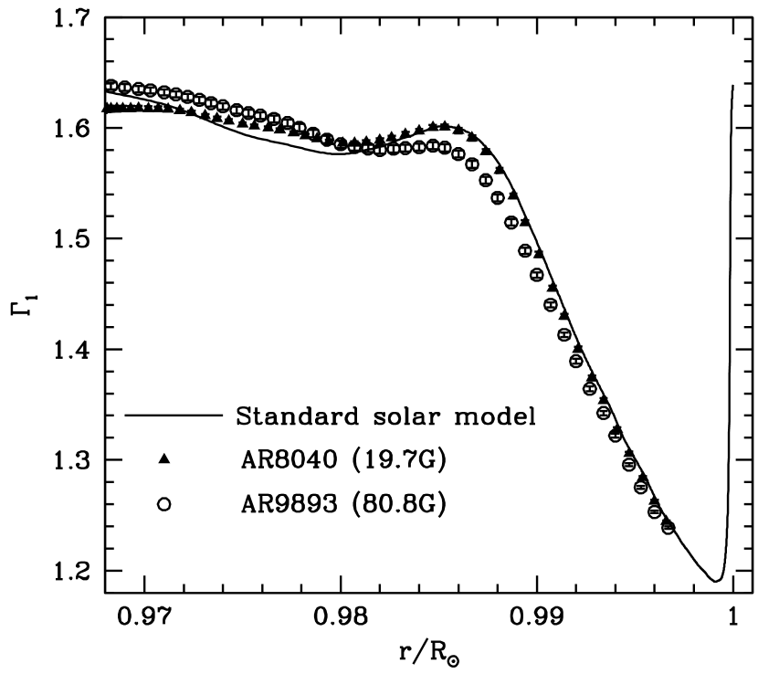
Figure 1: The adiabatic index $\Gamma_{1}$ for a standard solar model and two active regions. The region AR9893 is much stronger than AR 8040 and their magnetic indices as defined in Basu et al. (2004) are shown in the figures. The $\Gamma_{1}$ profiles for the active regions were determined from results of Basu et al. (2004) assuming that the $\Gamma_{1}$ profile of the quiet regions of the Sun is like that of a standard solar model. The results would not change appreciably if, instead of a standard solar model, $\Gamma_{1}$ obtained from inversions of quiet-sun data had been used.

There have been recent studies of solar active regions using local helioseismology techniques that suggest that active regions have lower sound speed compared with quiet regions just below the surface (Basu, et al. 2004; Kosovichev et al. 2000, 2001). It has also been shown by Basu et al. (2004) that the adiabatic index, $\Gamma_{1}$ of active regions is considerably different from that of quiet regions and the amount of change increases with increasing strength of the active region. Figure 1 shows the adiabatic index for two of the active regions studied by Basu et al. (2004), and one can see that the magnitude of the depression in $\Gamma_{1}$ at the second helium ionization zone decreases with increasing strength of the active region.

This leads us to question whether similar changes occur globally in the Sun as solar activity increases — of course one would expect the changes to be much smaller than those seen in active regions because global activity levels are much smaller than in active regions. Although the He II ionization zone is too shallow for studying temporal changes directly by inverting the currently available data sets, there are indirect ways by which we can study this region.

Any spherically symmetric localized, sharp feature or discontinuity in the Sun’s internal structure leaves a definite signature on the solar p-mode frequencies. Gough (1990) showed that abrupt changes of this type contribute a characteristic oscillatory component to the frequencies $\nu_{n,\ell}$ of those modes which penetrate below the localized perturbation. The amplitude of the oscillations increases with increasing “severity” of the discontinuity, and the wavelength of the oscillation is essentially the acoustic depth of the sharp-feature. Solar modes encounter two such features, the base of the convection zone (henceforth CZ) and the He II ionization zone. The transition of the temperature gradient from the adiabatic to radiative values at the CZ base gives rise to the oscillatory signal in frequencies of all modes which penetrate below the CZ base; the depression in the adiabatic index $\Gamma_{1}$ in the He II ionization zone causes the second signal. The two oscillatory signals have very different wavelengths and hence can be decoupled. Not all modes see both features, only low degree modes ($\ell\lesssim 25$) see the CZ base, higher degree modes only see the ionization zone, and the very high degree modes see neither. This signal has been used previously to study the CZ base (Monteiro, Christensen-Dalsgaard & Thompson 1994; Basu, Antia & Narasimha 1994), and also study changes in that region (Monteiro et al. 2000).

In this work we use the oscillatory signal from the depression in $\Gamma_{1}$ to study whether or not there are changes in $\Gamma_{1}$ in that region that are correlated with solar activity.

2 Technique

The amplitude of the signals from the CZ base as well as from the He II ionization zone are small, hence we first amplify them by taking the fourth differences of the frequencies:

$$\delta^{4}\nu_{n,\ell}=\nu_{n+2,\ell}-4\nu_{n+1,\ell}+6\nu_{n,\ell}-4\nu_{n-1,\ell}+\nu_{n-2,\ell}.$$ (1)

Taking the fourth differences amplifies the signals enough to be able to isolate them, keeping the errors at a manageable level (see Basu, Antia & Narasimha 1994 for a discussion).

The fourth differences can be fitted to the functional form given by Basu (1997):

$$\delta^{4}\nu =\left[a_{1}+a_{2}\nu+{(a_{3}+a_{4}L)/\nu^{2}}\right]\;+$$ (2)

$$\left(a_{5}+{a_{6}\over\nu_{m}^{2}}+{a_{7}L\over\nu_{m}^{2}}+{a_{8}L\over\nu_{m}^{4}}\right)\sin(2\nu_{m}\tau_{a}+\psi_{a})\;+$$

$$\left(b_{1}+{b_{2}\over\nu_{n}^{2}}+{b_{3}L\over\nu_{n}^{2}}+{b_{4}L\over\nu_{n}^{4}}\right)\sin(2\nu_{n}\tau_{b}+\psi_{b}),$$

where

$$L=\ell(\ell+1),\quad\nu_{m}=\nu-{{\gamma_{a}L}/{2\tau_{a}\nu}},\hbox{ and},\quad\nu_{n}=\nu-{{\gamma_{b}L}/{2\tau_{b}\nu}}.$$ (3)

The coefficients $a_{1}$–$a_{4}$ define an overall smooth term, $a_{5}$–$a_{8}$, $\tau_{a}$ and $\psi_{a}$ define the oscillatory contribution due to the He II ionization zone and the remaining terms define the oscillatory contribution from the CZ base. The frequencies of the two components, $\tau_{a}$ and $\tau_{b}$ are approximately the acoustic depths of the He II ionization zone and the CZ base respectively, but they also include a contribution from the frequency dependent part of the phases $\psi_{a}$ and $\psi_{b}$ which is not taken into account explicitly. The coefficients in this expression are determined by a least squares fit to the fourth differences.

We use oscillation frequencies determined by the Michelson Doppler Imager (MDI) on board the SOHO spacecraft, as well as data from the Global Oscillations Network Group (GONG). We have used 38 data sets from MDI (Schou 1999), each covering a period of 72 days starting from 1996 May 1 and ending on 2004 March 19. We use 28 data sets from GONG (Hill et al. 1996), each covering a period of 108 days, starting from 1995 May 7 and ending on 2003 August 16. As a measure of the solar activity for each data set, we use the mean radio flux at 10.7 cm during the time interval covered by each data set as obtained from the US National Geophysical Data Center (www.ngdc.noaa.gov/stp/stp.html).

For each data set we use modes with two sets of degrees; one set consists of modes with degree $5\leq\ell\leq 25$ and we refer to this as the low-degree set, the second set consists of all modes with $\ell\leq 60$ that have their lower turning point, $r_{t}>0.715$ R_⊙ and we refer to this as the intermediate-degree set. The lowest degree modes that satisfies this criterion for our frequency range of 2-3.5mHz is $\ell=30$. Very few modes below $\ell$ of 42 satisfy this criterion. The first set of modes sample both the CZ base and the He II ionization zone and hence we fit the entire form given by Eq. (2), while modes in the second set sample only the He II ionization zone and hence we fit the mode only to the first two terms of Eq. (2). We do not use modes with $\ell<5$ because they have larger errors. We do not use modes with degree higher than $\ell=60$ because the degree-dependence of the signal becomes difficult to model and fit.

The quantity we are most interested in is the amplitude of the oscillatory signal from He II ionization zone as a function of the magnetic activity level of the Sun when the data were obtained. Since the amplitude is both degree-dependent as well as frequency-dependent, we use the averaged amplitude in the frequency range 2 to 3.5mHz after the degree dependence is removed. This is the same as what was done by Basu et al. (1994), Basu & Antia (1994) and Basu (1997). The error on the result is determined by Monte-Carlo simulations. The fit to the signal from the He II ionization zone, after removal of the degree dependence, is shown in Fig. 2 for one set of low-degree GONG data.

3 Results

The amplitudes of the oscillatory signal that arises from the He II ionization zone are plotted as a function of the solar activity index in Fig. 3. The 10.7 cm flux is in units of the Solar Flux Unit (SFU), i.e., $10^{-22}$ J s^-1 m^-2 Hz^-1. We have plotted the four sets of data separately.

We find that in all cases, the amplitude decreases with increasing solar activity, a result that is expected if the active-region results can be applied to the global Sun. We can fit straight lines to the data quite easily — the large errors do not justify fitting more complicated trends. We can see that for all 4 sets, the straight line has a finite slope, however, the slope is not always statistically significant. This is particularly true for the GONG low-degree data. The MDI low-degree sets show only a marginally significant decrease. However, the intermediate-degree sets for both GONG and MDI show a reasonably significant trend ($\approx 4\sigma$). The scatter in the plots is somewhat less than what the errors on the points should suggest, so it is likely that the errors have been overestimated and significance of the slope underestimated.

It is not completely surprising that the low- and intermediate-degree sets give us somewhat different results. For the low-degree sets, we need to correctly remove the signal from the CZ base to get the correct amplitude from the He II ionization zone. Simulations performed with different solar models show that this process leads to substantial systematic errors in the results. The intermediate-degree modes are not affected by the CZ base at all, and hence the signal due to the He II zone is cleaner and easier to measure. Thus we put more weight on the results obtained from the intermediate degree modes.

Figure 4 shows both GONG and MDI intermediate-degree results plotted as a function of the 10.7 cm flux. It is clear that both GONG and MDI show very similar trends, which is encouraging since these are independent projects. A straight line fit to all the points shows that the slope is 5.5$\sigma$ from zero, a result that is reasonably statistically significant. We therefore, can conclude with a degree of confidence that the region of the He II ionization zone changes with change in solar activity. In particular, the magnitude of the dip in $\Gamma_{1}$, which is what causes the signal we are looking at, decreases with increasing activity. It should be noted however, that there should be a correlated noise component between the GONG and MDI data sets since they are observing the same object, hence the increase in the significance may be smaller than what we find on combining the results. A combination of all the results (GONG and MDI, low and intermediate-degree set) gives a slope significant at the 4.7$\sigma$ level.

4 Discussion

The easiest interpretation of a change in the magnitude of the depression of $\Gamma_{1}$ at the He II ionization zone is a change in the abundance of helium. However, that interpretation does not apply in this case, since we are talking of cyclical changes over very short time-scales. The only change in helium that is expected in the CZ is a monotonic decrease due to the gravitational settling of helium that takes place over very long time-scales. We need to look at the the equation of state (EOS) to understand the changes. The presence of magnetic fields can change the effective EOS because of contributions of the magnetic fields to energy and pressure. A change in the EOS changes the shape and magnitude of the dip in $\Gamma_{1}$ at the He II ionization zone for the same helium abundance.

Figure 5 shows the relative difference in $\Gamma_{1}$ between two solar envelope models, one constructed with the so-called MHD equation of state (Hummer & Mihalas 1988; Mihalas, Däppen & Hummer 1988; Däppen et al. 1988), and the second with the OPAL equation of state (Rogers, Swenson & Iglesias 1996). Both models were constructed with the same opacities, have identical helium and heavy element abundances in the CZ (0.242 and 0.018 respectively) and were constructed to have the same CZ depth (0.287R_⊙). We can see that the models have substantial differences in $\Gamma_{1}$ in the region of the He II ionization zone and higher. The amplitude of the He II signal for the MHD model is 1.164$\mu$Hz and that of the OPAL model is 1.027$\mu$Hz.

The difference between the He II amplitudes of the two models (0.137$\mu$Hz) is larger than the total range of change in amplitude seen in Fig. 4 (which is only $0.099\mu$Hz according to the linear fits to the results). Thus as a first approximation we can say that the change in $\Gamma_{1}$ near the solar helium ionization zone between solar minimum and maximum is less than that in Fig. 5, i.e., less than about 4%. However, one must be careful about this number; the $\Gamma_{1}$ differences in Fig. 5 have some fairly sharp features that could be the cause of the large difference in amplitude for the two models. It is unlikely that a small change in the EOS due to magnetic fields would cause spiky changes, and hence for $0.099\mu$Hz could imply a larger difference in $\Gamma_{1}$. Inversions could easily detect differences in $\Gamma_{1}$ less than the estimated $\Gamma_{1}$ change between solar minimum and solar maximum. However, to do so reliably, and with any degree of statistical significance, we need mode sets with reliable and precise high-degree modes (Di Mauro et al. 2002; Rabello-Soares et al. 2000).

As far as the parameter $\tau_{a}$ is concerned, we cannot draw any conclusions since as can be seen in Fig. 6, the points are widely scattered.

One expects solar cycle related changes to have strong latitudinal dependences. We repeated the study described above for different latitudes, but the errors are too large to be able to observe any latitudinal dependence.

5 Conclusions

We find evidence that suggests that solar structure changes with change in solar activity in the layers around the He II ionization zone (i.e., 0.98 R_⊙ and thereabouts). The depression in the adiabatic index $\Gamma_{1}$ in the He II ionization zone decreases with increasing solar activity. This is the first evidence to suggest that solar structure changes with solar activity.

Figure 2: The fourth-difference of frequencies of a set of GONG data with the degree-dependence in the signal removed. Also shown is a fit to the signal in the $\Gamma_{1}$ depression. Data for frequencies with $5\leq\ell\leq 25$ are shown.

Figure 3: The amplitude of the oscillatory signal averaged over the frequency range 2-3.5 mHz plotted as a function of the 10.7 cm radio flux, which is an indicator of solar activity. The 10.7 cm flux is plotted in units of $10^{-22}$ J s^-1 m^-2 Hz${-1}$ (Solar flux units). The different panels show the results of the different degree ranges of the GONG and MDI sets. The linear least squares fit to the points is shown as a continuous line. Each panel also lists how many standard deviations away the slope of the fitted line is away from zero.

Figure 4: The GONG and MDI results obtained for modes with $\ell\leq 60$ and $r_{t}>0.715$R_⊙ plotted as a function of the 10.7 cm flux. The black continuous line is a least-squares fit to all the data points. The dotted lines show the $1\sigma$ spread because of errors in the fitted parameters.

Figure 5: The relative difference in the adiabatic index $\Gamma_{1}$ between two solar envelope models, one constructed with the MHD and the other with the OPAL equation of state. The models were constructed with the same helium and heavy metal abundances and the same CZ depth.

Figure 6: The variation of $\tau_{a}$ as a function of the 10.7cm flux.

References

- Basu (1997) Basu, S. 1997, MNRAS 288, 572
- Basu (2002) Basu, S. 2002, in From Solar Min to Max: Half a Solar Cycle with SOHO, Proc. SOHO 11 Symposium, ed. A. Wilson, ESA SP-508, 7
- Basu & Antia (1994) Basu, S., Antia, H. M. 1994, MNRAS 269, 1137
- Basu & Antia (2000) Basu, S., Antia, H. M. 2000, ApJ, 541, 442
- Basu & Antia (2003) Basu, S., Antia, H. M., ApJ, 2003, 585, 553
- Basu et al. (1994) Basu, S., Antia, H. M., Narasimha, D. 1994, MNRAS 267,209
- Basu et al. (2004) Basu, S., Antia, H. M., Bogart, R. S. 2004, ApJ, 610. 1157
- Däppen et al. (1988) Däppen W., Mihalas D., Hummer D. G., Mihalas B. W. 1988, ApJ 332, 261
- Di Mauro et al. (2002) Di Mauro, M. P., Christensen-Dalsgaard, J., Rabello-Soares, M. C. and Basu, S. 2002, A&A 384, 666
- Eff-Darwich et al. (2002) Eff-Darwich, A., Korzennik, S. G., Jiménez-Reyes, S. J., Pérez Hernández 2002, ApJ, 580, 574
- Elsworth et al. (1990) Elsworth, Y., Howe, R., Isaak, G. R., McLeod, C. P., New, R. 1990, Nature, 345, 322
- Gough (1990) Gough, D. O. 1990, in Lecture Notes in Physics, eds., Y. Osaki, H. Shibahashi, (Springer: Berlin), vol. 367, p 283.
- Hill et al. (1996) Hill F., et al. 1996, Science 272, 1292
- Howe et al. (1999) Howe, R., Komm, R., Hill, F. 1999, ApJ, 524, 1084
- Howe et al. (2000) Howe, R., Christensen-Dalsgaard, J., Hill, F., Komm, R. W., Larsen, R. M., Schou, J., Thompson, M. J., Toomre, J. 2000, ApJ, 533, L163
- Hummer & Mihalas (1988) Hummer D. G., Mihalas D. 1988, ApJ 331, 794
- Libbrecht & Woodard (1990) Libbrecht, K. G., Woodard, M. F. 1990, Nature, 345, 779
- Miglio et al. (2003) Miglio, A., Christensen-Dalsgaard, J., di Mauro, M. P., Monteiro, M. J. P. F. G., Thompson, M. J. 2003, in Asteroseismology Across the HR Diagram, eds. M.J. Thompson, M.S. Cunha, M.J.P.F.G Monteiro (Kluwer:Dordrecht) p. 537
- Mihalas et al. (1988) Mihalas D., Däppen W., Hummer D. G. 1988, ApJ 331, 815
- Monteiro et a. (1994) Monteiro, M. J. P. F. G., Christensen-Dalsgaard, J., Thompson, M. J. 1994, A&A, 283, 247
- Monteiro et al. (2000) Monteiro, M. J. P. F. G., Christensen-Dalsgaard, J., Schou, J., Thompson, M. J. 2000, in Helio- and asteroseismology at the dawn of the millennium, Proc. SOHO 10/GONG 2000 Workshop, ed. A. Wilson, ESA SP-464, 535
- Kosovichev et al. (2000) Kosovichev, A. G., Duvall, T. L., Jr., Scherrer, P. H. 2000, Solar Phys., 192, 159
- Kosovichev et al. (2001) Kosovichev, A. G., Duvall, T. L., Jr., Birch, A. C., Gizon, L., Scherrer, P. H., Zhao, J. 2001, in Helio- and Asteroseismology at the Dawn of the Millennium, Proc. SOHO 10/GONG 2000 Workshop, ed., A. Wilson, ESA SP-464, 701
- Rabello-Soares et al. (2000) Rabello-Soares, M. C., Basu, S., Christensen-Dalsgaard, J., Di Mauro, M. P. 2000, Solar Phys. 193, 345
- Rogers et al. (1996) Rogers, F. J., Swenson, F. J., Iglesias, C. A. 1996, ApJ 456, 902
- Schou (1999) Schou J., 1999, ApJ 523, L181
- Vorontsov (2001) Vorontsov, S. V. 2001, in Helio- and Astero-seismology at the dawn of the millennium: Proc. SOHO 10/GONG 2000 Workshop, ed. A. Wilson, ESA SP-464, 563
- Vorontsov et al. (2002) Vorontsov, S. V., Christensen-Dalsgaard, J., Schou, J., Strakhov, V. N., Thompson, M. J. 2002, Science, 296. 101