Quantifying Substructure Using Galaxy-Galaxy Lensing in Distant Clusters

Abstract

We present high-resolution mass reconstructions for five massive cluster-lenses spanning a redshift range from $z=0.18$–0.57 utilizing archival Hubble Space Telescope (HST) data and applying galaxy-galaxy lensing techniques. These detailed mass models were obtained by combining constraints from the observed strong and weak lensing regimes. Quantifying the local weak distortions in the shear maps in terms of perturbations induced by the presence of galaxy halos around individual bright early-type cluster member galaxies, we estimate the fraction of mass in the central regions of these clusters that can be associated with small scale mass clumps. This technique enables us to directly map the substructure in the mass range $10^{11}$ – $10^{12.5}\,M_{\odot}$ which we associate with galaxy-scale sub-halos. The determination of the mass spectrum of substructure in the inner regions of these clusters is presented. Constraints are thereby obtained on the masses, mass-to-light ratios and truncation radii for these sub-halos. We find that the fraction of total cluster mass associated with individual sub-halos within the inner 0.5h^-1 – 0.8h^-1 Mpc of these clusters ranges from 10–20%. Our results have important implications for the survival and evolution of substructure in high density cluster cores and are consistent with the theoretical picture of tidal stripping of galaxy-scale halos in high-density cluster environments as expected in hierarchical Cold Dark Matter dominated structure formation scenarios.

1 Introduction

The detailed mass distribution within clusters and specifically the fraction of the total cluster mass associated with individual galaxies has important consequences for the frequency and nature of galaxy interactions (Merritt 1983; Moore et al. 1996; Ghigna et al. 1998; Okamato & Habe 1999) in clusters. Knowledge of the dynamical history of clusters enables a deeper understanding of the physical processes that shape their assembly and evolution. The discovery of strong evolution between $z\sim 0.5$ and the present-day in the morphological (and star-formation) properties of the galaxy populations in clusters has focused interest on environmental processes which could effect the gaseous component and dark matter halo of a cluster galaxy (e.g. Dressler et al. 1994, 1997; Couch et al. 1994, 1998).

The global tidal field of a massive, dense cluster potential well is expected to be strong enough to truncate the dark matter halo of a galaxy whose orbit penetrates the cluster core. Therefore, probing the tidally truncated extents of galaxy halos in clusters can provide invaluable clues to the dynamically dominant processes in clusters. For instance, the survival of individual, compact dark halos associated with cluster galaxies suggests a high probability for galaxy–galaxy collisions within rich clusters over a Hubble time. However, since the internal velocity dispersions of cluster galaxies ($\mathrel{\raise 1.50696pt\hbox{$\scriptstyle<$}\kern-6.00006pt\lower 1.72218pt\hbox{$\scriptstyle\sim$}}200$ km s^-1) are significantly lower than their orbital velocities, these interactions are, in general, unlikely to lead to mergers, suggesting that the encounters of the kind simulated in the galaxy harassment picture by Moore et al. (1996, 1998) are most frequent. It is likely that tidal stripping in clusters will lead to morphological transformations.

Gravitational lensing has emerged as one of the most powerful techniques to map mass distributions on a range of scales: galaxies, clusters and beyond. The distortion in the shapes of background galaxies viewed through fore-ground mass distributions is independent of the dynamical state of the lens, therefore, unlike other methods for mass estimation there are fewer biases in lensing mass determinations. Here, we focus on mapping in detail the mass distribution inside the inner regions of massive clusters of galaxies using Hubble Space Telescope (HST) observations. We exploit the technique of galaxy-galaxy lensing, which was originally proposed as a method to constrain the masses and spatial extents of field galaxies (Brainerd, Blandford & Smail 1996), which we have since extended and developed to apply inside clusters (Natarajan & Kneib 1996; Natarajan et al. 1998; 2002a). We begin by summarizing current results of applying galaxy-galaxy lensing to field galaxies and the outline the constraints obtained on their masses and halo sizes.

Recent work on galaxy-galaxy lensing in the moderate redshift field has identified a signal associated with massive halos around typical field galaxies, extending to beyond 100 kpc (e.g. Brainerd, Blandford & Smail 1996; Ebbels et al. 2000; Hudson et al. 1998; Hoekstra et al. 2004). In particular, Hoekstra et al. (2004) report the detection of finite truncation radii via weak lensing by galaxies based on 45.5 deg² of imaging data from the Red-Sequence Cluster Survey. Using a truncated isothermal sphere to model the mass in galaxy halos, they find a best-fit central velocity dispersion for an $L^{*}$ galaxy of $\sigma=136\pm 5$ kms^-1 (68% confidence limits) and a truncation radius of $185\pm 30$ kpc (for $h=0.7$ and $\Omega_{\Lambda}=0.7$). Similar analysis of galaxies in the cores of rich clusters suggests that the average mass-to-light ratio and spatial extents of the dark matter halos associated with morphologically-classified early-type galaxies in these regions may differ from those of comparable luminosity field galaxies (Natarajan et al. 1998, 2002a). We find that at a given luminosity, galaxies in clusters have more compact halo sizes and lower masses (by a factor of 2–5) compared to their field counter-parts. The mass-to-light ratios inferred for cluster galaxies in the V-band are also lower than that of comparable luminosity field galaxies. This is a strong indication of the effect of the dense environment on the properties of dark matter halos. It is likely that tidal stripping inside clusters might lead to morphological transformations as well.

In this paper, we present the determination of the mass function of substructure in clusters using galaxy-galaxy lensing techniques. A high resolution mass model tightly constrained by strong and weak lensing observations is constructed including individual cluster galaxies and their associated dark matter halos. We show that over a limited mass range we can successfully construct the mass function of sub-halos inside clusters. At the moment only theoretical determinations are available from high resolution cosmological N-body simulations. Accordingly the sub-halo mass function is an important prediction of hierarchical Cold Dark Matter structure formation models. This innovative application of gravitational lensing enables computation of the sub-halo mass function directly from observational data.

The strength of the lensing analysis presented here is the combination of observed constraints from both strong and weak lensing features which are used to construct a high resolution mass map of a galaxy cluster. Anisotropies in the shear field (i.e. departure from the coherent tangential signal) in the vicinity of bright, early-type cluster members are attributed to the presence of these local potential wells. Statistically stacking this signal provides a way to quantify the masses associated with individual galaxy halos. This is accomplished using a maximum likelihood estimator to retrieve characteristic properties for a typical sub-halo in the cluster.

The outline of this paper is as follows: in §2, we describe the formalism for analyzing galaxy-galaxy lensing in clusters including a synopsis of the adopted models, §3 discusses the properties of the clusters analyzed here. We present the best-fit lens models in §4 and discuss the sources of noise in §5. The results on sub-halo properties, in particular the sub-halo mass spectrum is presented in detail in §6. In §7 we discuss the future prospects of this technique and present the conclusions of our work.

2 Galaxy-galaxy lensing in clusters

2.1 Framework for analysis

For the purpose of extracting the properties of the sub-halo population in clusters, a range of mass scales is modeled parametrically. The X-ray surface brightness maps of these clusters suggests the presence of a smooth, dominant, large scale mass component. Clusters are therefore modeled as a super-position of a smooth large-scale potential and smaller scale potentials that are associated with bright early-type cluster members:

$$\phi_{\rm tot}=\phi_{\rm c}+\Sigma_{i}\,\phi_{\rm p_{i}},$$ (1)

where $\phi_{\rm clus}$ is the potential of the smooth component and $\phi_{\rm p_{i}}$ are the potentials of the perturbers (galaxy sub-halos). The corresponding deflection angle $\alpha_{I}$ and the amplification matrix $A^{-1}$ can also be decomposed into contributions from the main clump and perturbers,

$$\alpha_{I}\,=\,{{\mathbf{\nabla}}\phi_{\rm c}}\,+\,\Sigma_{i}\,{{\mathbf{\nabla}}\phi_{\rm p_{i}}},\,\,\,A^{-1}\,=\,I\,-\,{{\mathbf{\nabla}\nabla}{\phi_{\rm c}}}\,-\,\Sigma_{i}\,{{\mathbf{\nabla}\nabla}{\phi_{\rm p_{i}}}}.$$ (2)

Defining the generic symmetry matrix,

$$J_{2\theta}\,=\,\left(\begin{array}[]{lr}\cos{2\theta}&\sin{2\theta}\\ \sin{2\theta}&-\cos{2\theta}\\ \end{array}\right)$$

we can decompose the amplification matrix above as a direct and linear sum:

$$A^{-1}\,=\,(1\,-\,\kappa_{\rm c}\,-\,\Sigma_{i}\kappa_{\rm p})\,I-\gamma_{\rm c}J_{2\theta_{\rm c}}-\Sigma_{i}\,\gamma_{\rm p_{i}}J_{2\theta_{\rm p_{i}}},$$ (3)

where $\kappa$ is the magnification and $\gamma$ the shear. The shear $\gamma$ is in fact a complex number and is used to define the quantity $\overline{g}$ the reduced shear which is determined directly from observations of the shapes of background galaxies:

$$\overline{g_{tot}}={\overline{\gamma}\over 1-\kappa}={{\overline{\gamma}_{c}}+\Sigma_{i}\,{\overline{\gamma}_{p_{i}}}\over 1-\kappa_{c}-\Sigma_{i}\,\kappa_{p_{i}}},$$ (4)

which simplifies in the coordinate system defined with respect to the perturber $j$ to (neglecting effect of perturber $i$ if $i\neq j$):

(5)

where $\overline{g}_{tot}|_{j}$ is the total complex shear induced by the smooth cluster component and the potentials of the perturbers. Restricting our analysis to the weak regime, and thereby retaining only the first order terms from the lensing equation for the shape parameters (e.g. Kneib et al. 1996) we have:

$${\overline{g}_{I}}={\overline{g}_{S}}+{\overline{g}_{tot}},$$ (6)

where ${\overline{g}_{I}}=\frac{(a-b)}{(a+b)}\,e^{2i\theta}$ is the distortion of the image, ${\overline{g}_{S}}$ the intrinsic shape of the source, ${\overline{g}_{\rm tot}}$ is the distortion induced by the lensing potentials (eqn. 4).

In the vicinity of perturber $j$ which is then the dominant mass contribution:

$$\kappa_{p_{j}}>>\kappa_{p_{i}}{\rm for}i\neq j$$ (7)

thus,

$${\overline{g}_{I}}={\overline{g}_{S}}+{\overline{g}_{tot}}|_{j}={\overline{g}_{S}}+{{\overline{\gamma}_{c}}\over 1-\kappa_{c}-\kappa_{p_{j}}}+{{\overline{\gamma}_{p_{j}}}\over 1-\kappa_{c}-\kappa_{p_{j}}}.$$ (8)

In the local frame of reference of the perturbers, the mean value of the quantity ${\overline{g}_{I}}$ and its dispersion can be computed in circular annuli (at radius $r$ from the perturber center) strictly in the weak-regime, assuming a constant value $\gamma_{c}e^{i\theta_{c}}$ for the smooth cluster component over the area of integration. In the frame of the perturber, the averaging procedure allows efficient subtraction of the large-scale component, enabling the extraction of the shear component induced in the background galaxies only by the local perturber. The background galaxies are assumed to have intrinsic ellipticities drawn from a known distribution (see the next section for further details). Schematically the effect of the cluster on the intrinsic ellipticity distribution of background sources is to cause a coherent displacement ${\tau}$ and the presence of perturbers merely adds small-scale noise to the observed ellipticity distribution.

The feasibility of signal detection can be estimated by computing the dispersion in the shear and hence the signal-to-noise ratio. Averaging eqn. (7) in cartesian coordinates (averaging out the contribution of the perturbers):

$$\left<{\overline{g}_{I}}\right>_{xy} = \left<{\overline{g}_{S}}\right>+\left<{\gamma_{c}e^{i\theta_{c}}\over 1-\kappa_{c}-\kappa_{p_{j}}}\right>+\left<{{\overline{\gamma}_{p_{j}}}\over 1-\kappa_{c}-\kappa_{p_{j}}}\right>,$$

$$= {\gamma_{c}e^{i\theta_{c}}}\left<{1\over 1-\kappa_{c}-\kappa_{p_{j}}}\right>\equiv{\overline{g}_{c}},$$

$$\sigma^{2}_{\overline{g}_{I}}={\sigma^{2}_{\overline{g}_{S}}\over 2}+{\sigma^{2}_{\overline{g}_{p_{j}}}\over 2},$$ (10)

where

$$\sigma^{2}_{g_{I}}\,\approx\,{\sigma^{2}_{p(\tau_{S})}\over 2N_{bg}}+{\sigma^{2}_{\overline{g}_{p_{j}}}\over 2N_{bg}}\,\approx\,{\sigma^{2}_{p(\tau_{S})}\over 2N_{bg}}$$ (11)

${\sigma^{2}_{p(\tau_{S})}}$ being the width of the intrinsic ellipticity distribution of the sources, $N_{bg}$ the number of background galaxies averaged over and $\sigma^{2}_{\overline{g}_{p_{j}}}$ the dispersion due to perturber effects which should be smaller than the width of the intrinsic ellipticity distribution. A more apt choice of coordinate system, the polar $(u,v)$ provides the optimal measure. On averaging out the smooth component, we have in polar coordinates:

$$\left<{\overline{g}_{I}}\right>_{uv} = \left<{\overline{g}_{S}}\right>+\left<{{\overline{\gamma}_{c}}\over 1-\kappa_{c}-\kappa_{p_{j}}}\right>+\left<{\gamma_{p_{j}}\over 1-\kappa_{c}-\kappa_{p_{j}}}\right>,$$

$$= {\gamma_{p_{j}}}\left<{1\over{1-\kappa_{c}-\kappa_{p_{j}}}}\right>\equiv g_{p_{j}},$$

$$\left(\sigma^{2}_{\overline{g_{I}}}\right)_{uv}={{\sigma^{2}_{\overline{g}_{S}}}\over 2}+{{\sigma^{2}_{\overline{g}_{c}}}\over 2},$$ (13)

where

$$\sigma^{2}_{g_{I}}\,\approx\,{\sigma^{2}_{p(\tau_{S})}\over 2N_{bg}}+{\sigma^{2}_{\overline{g}_{c}}\over 2N_{bg}}.$$ (14)

From these equations, we clearly see the two effects of the contribution of the smooth cluster component: it boosts the shear induced by the perturber due to the ($\kappa_{c}+\kappa_{p_{j}}$) term in the denominator, which becomes non-negligible in the cluster center, and it simultaneously dilutes the regular galaxy-galaxy lensing signal due to the ${\sigma^{2}_{\overline{g}_{c}}/2}$ term in the dispersion of the polarization measure. However, one can in principle optimize the noise in the polarization by ‘subtracting’ the measured cluster signal ${\overline{g}_{c}}$ using a fitted parametric model for the cluster and averaging in polar coordinates:

$$\left<{\overline{g}_{I}}-{\overline{g}_{c}}\right>_{uv}=\left<{\gamma_{p_{j}}\over 1-\kappa_{c}-\kappa_{p_{j}}}\right>,$$ (15)

which gives the same mean value as above but with a reduced dispersion:

$$\left(\sigma^{2}_{\overline{g}_{I}-\overline{g}_{c}}\right)_{uv}={\sigma^{2}_{\overline{g}_{S}}\over 2},$$ (16)

where

$$\sigma_{g_{S}}^{2}\,\approx\,{\sigma^{2}_{p(\tau_{S})}\over 2N_{bg}}.$$ (17)

This subtraction of the larger-scale component reduces the noise in the polarization measure, by about a factor of two; when $\sigma^{2}_{\overline{g}_{S}}\sim\sigma^{2}_{\overline{g}_{c}}$, which is the case in cluster cores. This differenced averaging prescription for extracting the distortions induced by the possible presence of dark halos around cluster galaxies is very feasible with HST quality data as we have shown in earlier work (Natarajan et al. 1998, 2002a).

Note here that it is the presence of the underlying large-scale smooth mass distribution (with a high value of $\kappa_{c}$) that enables the extraction of the weak signal riding on it. It is instructive to keep in mind that in the regimes of interest discussed here the distortion induced by the cluster-scale smooth component for a PIEMD model in the inner-most (with a velocity dispersion of $1000\,{\rm kms}^{-1}$ and at $R/r_{t}\leq 0.1$) regions is typically of the order of 20 - 40% or so in background galaxy shapes, and the perturbers produce distortions (smaller scale PIEMDs with a velocity dispersion of $220\,{\rm kms}^{-1}$) of the order of 5 - 10%, significantly more than in the case of weak-lensing by large scale structure or cosmic shear wherein the distortions are of the order of 1% percent.

2.2 Modeling the cluster

Each of the clusters studied in this paper preferentially probes the high mass end of the cluster mass function and has a surface mass density in the inner regions which is higher than the critical value, therefore producing a number of multiple images of background sources. By definition, the critical surface mass density for strong lensing is given by:

$$\Sigma_{\rm crit}={\frac{c^{2}}{4\pi G}}\frac{D_{s}}{D_{d}D_{ds}}$$ (18)

where $D_{s}$ the angular diameter distance between the observer and the source, $D_{d}$ the angular diameter distance between the observer and the deflecting lens and $D_{ds}$ the angular diameter distance between the deflector and the source. When the surface mass density in the cluster is in excess of this critical value, strong lensing phenomena with high magnification are observed.

In general two types of lensing effects are produced – strong: multiple images and highly distorted arcs; and weak: small distortion in background image shapes determined by the criticality of the region. Viewed through the central, dense core region of the mass distribution, where $\kappa>1$ strongly lensed features are observed. Note that the integrated lensing signal detected is due to all the mass distributed along the line of sight in a cylinder projected onto the lens plane. In this and all other cluster lensing work, the assumption is made that individual clusters dominate the lensing signal as the probability of encountering two massive rich clusters along the same line-of-sight is extremely small due to the fact that these are very rare objects in hierarchical structure formation models.

With our current sensitivity limits, galaxy-galaxy lensing within the cluster is primarily a tool to determine the total enclosed mass within an aperture. We lack sufficient sensitivity to constrain the detailed mass profile for individual cluster galaxies. With higher resolution data in the near future we will be able to obtain constraints on the slopes of mass profiles in sub-halos. In this paper, we therefore concentrate on pseudo-isothermal elliptical components (PIEMD models, derived by Kassiola & Kovner 1993) appropriately scaled for both the main cluster and the substructure. We find that the results obtained for the characteristics of the sub-halos (or perturbers) is largely independent of the form of the mass distribution used to model the smooth, large-scale component. A detailed comparison of the best-fit profiles from lensing directly with those obtained in high resolution cosmological N-body simulations is outside the scope of this paper and will be presented elsewhere.

To quantify the lensing distortion induced by the global potential, both the smooth and individual galaxy-scale halos are modeled self-similarly using a surface density profile, $\Sigma(R)$ which is a linear superposition of two PIEMD distributions,

$$\Sigma(R)\,=\,{\Sigma_{0}r_{0}\over{1-r_{0}/r_{t}}}({1\over\sqrt{r_{0}^{2}+R^{2}}}\,-\,{1\over\sqrt{r_{t}^{2}+R^{2}}}),$$ (19)

with a model core-radius $r_{0}$ and a truncation radius $r_{t}\,\gg\,r_{0}$. Correlating the above mass profile with a typical de Vaucleours light profile (the observed profile for bright early type galaxies) provides a simple relation between the truncation radius and the effective radius $R_{\rm e}$, $r_{t}\sim(4/3)R_{\rm e}$. These parameters $(r_{t},r_{0})$ are tuned for both the smooth component and the perturbers to obtain mass distributions on the relevant scales. The coordinate $R$ is a function of $x$, $y$ and the ellipticity,

$$R^{2}\,=\,({x^{2}\over(1+\epsilon)^{2}}\,+\,{y^{2}\over(1-\epsilon)^{2}})\,;\ \ \epsilon={a-b\over a+b},$$ (20)

The mass enclosed within radius $R$ for the $\epsilon=0$ model is given by:

$$M(R)={2\pi\Sigma_{0}r_{0}\over{1-{{r_{0}}\over{r_{t}}}}}[\,\sqrt{r_{0}^{2}+R^{2}}\,-\,\sqrt{r_{t}^{2}+R^{2}}\,+\,(r_{t}-r_{0})\,].$$ (21)

One of the attractive features of this model is that the total mass ${M_{\infty}}$, is finite ${M_{\infty}}\propto\,{\Sigma_{0}}{r_{0}}{r_{t}}$. Besides, analytic expressions can be obtained for the all the quantities of interest, $\kappa$, $\gamma$ and $g$,

$$\kappa(R)\,=\,{\kappa_{0}}\,{{r_{0}}\over{(1-{r_{0}/r_{t}})}}\,({1\over{\sqrt{({r_{0}^{2}}+{R^{2}})}}}\,-\,{1\over{\sqrt{({r_{t}^{2}}+{R^{2}})}}})\,\,\,,$$ (22)

$$2\kappa_{0}\,=\,\Sigma_{0}\,{4\pi G\over c^{2}}\,{D_{\rm ls}D_{\rm ol}\over D_{\rm os}},$$ (23)

where $D_{\rm ls}$, $D_{\rm os}$ and $D_{\rm ol}$ are respectively the lens-source, observer-source and observer-lens angular diameter distances which do depend on the choice of cosmological parameters. To obtain $g(R)$, knowing the magnification $\kappa(R)$, we solve Laplace’s equation for the projected potential $\phi_{\rm 2D}$, evaluate the components of the amplification matrix and then proceed to solve directly for $\gamma(R)$, and then $g(R)$. This yields for the projected potential,

$$\phi_{2D}\, = \,2{\kappa_{0}}[\sqrt{r_{0}^{2}+R^{2}}\,-\,\sqrt{r_{t}^{2}+R^{2}}\,+(r_{0}-r_{t})\ln R\,$$

$$- \,r_{0}\ln\,[r_{0}^{2}+r_{0}\sqrt{r_{0}^{2}+R^{2}}]\,+\,r_{t}\ln\,[r_{t}^{2}+r_{t}\sqrt{r_{t}^{2}+R^{2}}]].$$

And,

$$\gamma(R)\, = \,\kappa_{0}[\,-{1\over\sqrt{R^{2}+r_{0}^{2}}}\,+\,{2\over R^{2}}(\sqrt{R^{2}+r_{0}^{2}}-r_{0})\,$$

$$+ \,{1\over{\sqrt{R^{2}+r_{t}^{2}}}}\,-\,{2\over R^{2}}(\sqrt{R^{2}+r_{t}^{2}}-r_{t})\,].$$

(then following equation 4, we can compute g(R)). Scaling this relation by $r_{t}$ gives for $r_{0}<R<r_{t}$:

$$\gamma(R/r_{t})\propto{\Sigma_{0}\over\eta-1}{{r_{t}}\over R}\,\sim\,{\sigma^{2}\over R},$$ (26)

where $\sigma$ is the velocity dispersion and for $r_{0}<r_{t}<R$:

$$\gamma(R/r_{t})\propto{\Sigma_{0}\over\eta}{{r_{t}}^{2}\over R^{2}}\,\sim\,{{M_{\rm tot}}\over{R^{2}}},$$ (27)

where ${M_{\rm tot}}$ is the total mass. In the limit that $R\,\gg\,r_{t}$, we have,

$$\gamma(R)\,=\,{{3\kappa_{0}}\over{2{R^{3}}}}\,[{r_{0}^{2}}\,-\,{r_{t}^{2}}]\,+\,{{2{\kappa_{0}}}\over{R^{2}}}[{{r_{t}}\,-\,{r_{0}}}],$$ (28)

and as ${R\,\to\,\infty}$, $\gamma(R)\,\to\,0$, $g(R)\,\to\,0$ and $\tau(R)\,\to\,0$ as expected.

Additionally, in order to relate the light distribution to key parameters of the mass model above, we adopt a set of physically motivated scaling laws for the cluster galaxies (Brainerd et al. 1996):

$${\sigma_{0}}\,=\,{\sigma_{0*}}({L\over L^{*}})^{1\over 4};\,\,{r_{0}}\,=\,{r_{0*}}{({L\over L^{*}})^{1\over 2}};\,\,{r_{t}}\,=\,{r_{t*}}{({L\over L^{*}})^{\alpha}}.$$ (29)

These in turn imply the following scaling for the $r_{t}/r_{0}$ ratio $\eta$:

$${\eta}\,=\,{r_{t}\over r_{0}}={{r_{t*}}\over{r_{0*}}}({L\over L^{*}})^{\alpha-1/2}.$$ (30)

The total mass $M_{\rm ap}$ enclosed within an aperture $r_{t*}$ and the total mass-to-light ratio $M/L$ then scale with the luminosity as follows:

$$M_{\rm ap}\,\propto\,{\sigma_{0*}^{2}}{r_{t*}}\,({L\over L^{*}})^{{1\over 2}+\alpha},\,\,{M/L}\,\propto\,{\sigma_{0*}^{2}}\,{r_{t*}}\left({L\over L^{*}}\right)^{\alpha-1/2},$$ (31)

where $\alpha$ tunes the size of the galaxy halo and for $\alpha$ = 0.5 the assumed galaxy model has constant $M/L$ with luminosity (but not as a function of radius) for each galaxy; if $\alpha>$ 0.5 ($\alpha<$ 0.5) then brighter galaxies have a larger (smaller) halos than the fainter ones. These scaling laws were empirically motivated by the Faber-Jackson relation for early-type galaxies (Brainerd, Blandford & Smail 1996). We assume these scaling relations and recognize that this could ultimately be a limitation but the evidence at hand supports the fact that mass traces light efficiently both on cluster scales (Kneib et al. 2003) and on galaxy scales (McKay et al. 2001; Wilson et al. 2001) We also explore the dependence of the retrieved characteristic halo parameters on the choice of the scaling index $\alpha$ for the most tightly constrained lens model in our sample, that of A 2218..

2.2.1 The intrinsic shape distribution of background galaxies

As in all lensing work, it is assumed here as well, that the intrinsic or undistorted distribution of shapes of galaxies is known. This distribution is obtained from shape measurements taken from deep images of blank field surveys. Previous analysis of deep survey data such as the MDS fields (Griffiths et al. 1994) showed that the ellipticity distribution of sources is a strong function of the sizes of individual galaxies as well as their magnitude (Kneib et al. 1996). For the purposes of our modeling, the intrinsic ellipticities for background galaxies are assigned in concordance with an ellipticity distribution $p_{(}\tau_{S})$ where the shape parameter $\tau$ is defined as $\tau=(a^{2}-b^{2})/(2ab)$ derived from the observed ellipticities of the CFHT12k data (see Limousin et al. 2004 for details):

$$p(\tau_{S})\,=\,\tau_{S}\,\,\exp(-({\tau_{S}\over\delta})^{\nu});\,\,\,\nu\,=\,1.15,\,\,\delta\,=\,0.25.$$ (32)

Note that this distribution includes accurately measured shapes of galaxies of all morphological types. In the likelihood analysis this distribution $p(\tau_{S})$ is the assumed prior, which is used to compare with the observed shapes once the effects of the assumed mass model are removed from the background images. We note here that the exact shape of the ellipticity distribution, i.e. the functional form and the value of $\delta$ and $\nu$ do not change the results, but alter the confidence levels we obtain. The width of the intrinsic ellipticity distribution, on the other hand is the fundamental limiting factor in the accuracy of all lensing measurements.

2.2.2 The redshift distribution of background galaxies

While the shapes of lensed background galaxies can be measured directly and reliably by extracting the second moment of the light distribution, in general, the precise redshift for each weakly object is in fact unknown and therefore needs to be assumed. Using multi-waveband data from surveys such as COMBO-17 (Wolf et al. 2004) photometric redshift estimates can be obtained for every background object. Typically the redshift distribution of background galaxies is modeled as a function of observed magnitude $P(z,m)$. We have used data from the high-redshift survey VIMOS VLT Deep Survey (Le Fevre et al. 2004) as well as recent CFHT12k R-band data to define the number counts of galaxies, and the HDF prescription for the mean redshift per magnitude bin, and find that the simple parameterization of the redshift distribution used by Brainerd, Blandford & Smail (1996) still provides a good description to the data.

For the normalized redshift distribution at a given magnitude $m$ (in the given band) we therefore have:

$$N(z)|_{m}\,=\,{{\beta\,({{z^{2}}\over{z_{0}^{2}}})\,\exp(-({z\over{z_{0}}})^{\beta})}\over{\Gamma({3\over\beta})\,{{z_{0}}}}};$$ (33)

where $\beta\,=\,$1.5 and

$$z_{0}\,=\,0.7\,[\,{z_{\rm median}}\,+\,{{d{z_{\rm median}}}\over{dm_{R}}}{(m_{R}\,-\,{m_{R0}})}\,],$$ (34)

${z_{\rm median}}$ being the median redshift, $dz_{\rm median}/dm_{R}$ the change in median redshift with say the $R$-band magnitude, $m_{R}$.

However, we note here in agreement with another recent study of galaxy-galaxy lensing in the field by Kleinheinrich et al. (2004), that the final results on the aperture mass are also sensitive primarily only to the choice of the median redshift of the distribution rather than the individual assigned values.

2.3 The maximum-likelihood method

Parameters that characterize both the global component and the perturbers are optimized, using the observed strong lensing features - positions, magnitudes, geometry of multiple images and measured spectroscopic redshifts, when known, along with the smoothed shear field as constraints. Note that from the above parameterization presented in the previous section, it is clear that we can optimize and extract values for $(\sigma_{0*},r_{t*})$ for a typical $L^{*}$ cluster galaxy.

A maximum-likelihood estimator is used to obtain significance bounds on fiducial parameters that characterize a typical $L^{*}$ sub-halo in the cluster. We have extended the prescription proposed by Schneider & Rix (1996) for galaxy-galaxy lensing in the field to the case of lensing by galaxy sub-halos in the cluster (Natarajan & Kneib 1997, Natarajan et al 1998). The likelihood function of the estimated probability distribution of the source ellipticities is maximized for a set of model parameters, given a functional form of the intrinsic ellipticity distribution measured for faint galaxies. For each ‘faint’ galaxy $j$, with measured shape $\tau_{\rm obs}$, the intrinsic shape $\tau_{S_{j}}$ is estimated in the weak regime by subtracting the lensing distortion induced by the smooth cluster model and the galaxy sub-halos,

$$\tau_{S_{j}}\,=\,\tau_{\rm obs_{j}}\,-{\Sigma_{i}^{N_{c}}}\,{\gamma_{p_{i}}}\,-\,\gamma_{c},$$ (35)

where $\Sigma_{i}^{N_{c}}\,{\gamma_{p_{i}}}$ is the sum of the shear contribution at a given position $j$ from $N_{c}$ perturbers. This entire inversion procedure is performed for each cluster within the lens tool utilities developed originally by Kneib (1993), which accurately takes into account the non-linearities arising in the strong regime. Using a well-determined ‘strong lensing’ model for the inner-regions of the clusters derived from the positions, shapes and magnitudes of the highly distorted multiply-imaged objects along with the shear field determined from the shapes of the weakly distorted background galaxies and assuming a known functional form for $p(\tau_{S})$ the probability distribution for the intrinsic shape distribution of galaxies in the field, the likelihood for a guessed model is given by,

$${\cal L}({{\sigma_{0*}}},{r_{t*}})=\Pi_{j}^{N_{gal}}p(\tau_{S_{j}}),$$ (36)

where the marginalization is done over $(\sigma_{0*},r_{t*})$. We compute ${\cal L}$ assigning the median redshift corresponding to the observed source magnitude for each arclet. The best fitting model parameters are then obtained by maximizing the log-likelihood function $l$ with respect to the parameters ${\sigma_{0*}}$ and ${r_{t*}}$. Note that the parameters that characterize the smooth component are also simultaneously optimized. The likelihood can also be marginalized over a complementary pair of parameters, i.e. $\alpha$ the luminosity scaling index and the aperture mass $M_{\rm ap}$ directly. In this work, we explore both choices.

2.4 The mass function of substructure in the inner regions

Mapping of the substructure mass function is ultimately of interest since it intimately connects to the galaxy formation process. Comparison of the dark halo mass function with the observed luminosity function of galaxies provides valuable insights into the process of assembly of galaxies. Substructures in the dark matter are defined to be lower mass clumps that are dynamically distinct, and bound objects that reside inside a virialized dark matter halo. The existence of substructure is a generic prediction of hierarchical structure formation in CDM models. The assembly of collapsed mass in these models proceeds via the gravitational amplification of initial density fluctuations resulting in dark halos that are not smooth and structureless but rather clumpy with significant amounts of substructure. For instance, within a radius of $400\,h^{-2}\,{\rm kpc}$, from the Milky Way, cosmological models of structure formation predict $\sim$ 50 dark matter satellites with circular velocities in excess of $50\,{\rm kms^{-1}}$ and mass greater than $3\,\times\,10^{8}\,M_{\odot}$. This number is significantly higher than the dozen or so satellites actually observed around our Galaxy. If we extend the analysis to the Local Group the problem gets worse, as $\sim$ 300 satellites are predicted inside a $1.5\,{\rm Mpc}$ radius whereas only about 40 are detected. However, the observed VDF (velocity distribution function) and the predicted VDF do match up at $v_{\rm circ}=50\,{\rm kms^{-1}}$, indicating that the abundance of satellites is a problem on small scales (Klypin et al. 2002). On small scales, $M\,<\,10^{8}\,M_{\odot}$ or so, there is a marked discrepancy between the theoretical/N-body simulation prediction for the amount of substructure that is observed in the Universe. A surfeit of sub-halos (satellites) are predicted for a galaxy like the Milky Way, when only a handful are detected. There are several possible explanations for this discrepancy including (i) possible identification of some satellites with the detected High Velocity Clouds (HVCs) and (ii) physical processes inhibiting star formation preferentially in low mass halos implying the existence of large numbers of dark satellites. If the vast number of sub-halos are dark, lensing might be the best way to detect them.

Recently Lee (2004) has attempted an analytic calculation of the sub-halo mass function inside clusters for CDM models and finds that $n(M)\,\propto\,{M^{-0.8}}$ over the mass range $10^{11}$–$10^{12.5}\,M_{\odot}$. Lee (2004) takes into account the complex dynamical history of galaxies in the cluster using one parameter to model the effect of global tidal truncation. Therefore, adopting the simple tidal-limit approximation to estimate analytically the global and local mass distribution of dark matter halos that undergo tidal mass-loss, Lee (2004) finds that the resulting mass functions are in excellent agreement with what has been found in recent N-body simulations. We have also demonstrated that the spatial extent inferred from galaxy-galaxy lensing are consistent with the tidal stripping hypothesis (see Natarajan et al. 2002a). Similar to our results here, Lee also finds that only about 10% of the sub-halo mass is in this mass range. Numerical studies by De Lucia et al. (2004) find that the substructure mass function depends only weakly on the properties of the parent halo mass, and is well described by a power law. The mass fraction in substructure also appears to be relatively insensitive to the tilt and overall normalization of the primordial power spectrum (Zentner & Bullock 2003).

3 Lensing Analysis of Clusters

We briefly discuss the properties of the five lensing clusters that are studied here. The clusters in order of increasing redshift are: A 2218, $z=0.18$; A 2390, $z=0.23$; Cl 2244$-$02, $z=0.33$; Cl 0024+16, $z=0.39$; Cl 0054$-$27, $z=0.57$. All clusters have multiply imaged background sources (some with several sets of multiply-imaged sources) with measured spectroscopic redshifts that are used to calibrate the overall mass model. In addition to these five clusters we will also include the results from our previous analysis of the rich cluster AC 114 at $z=0.31$ described in Natarajan et al. (1998). The HST WFPC2 imaging of this cluster was analyzed and modeled in an identical manner to that used here and hence allowing those results to be included in our discussion.

The X-ray and lensing properties of three of the clusters analyzed here (A 2218, Cl 0024+16 and Cl 0054$-$27) were discussed by Smail et al. (1997b) based on the data available at that time. We summarize the information from more recent observations of these clusters, as well as the two remaining systems (A 2390 and Cl 2244$-$02) below. The clusters range over an order of magnitude in terms of their X-ray luminosity ($L_{\rm X}\sim 10^{43-44}h^{-2}$ erg s^-1) and roughly an order of magnitude in terms of their $V$-band luminosities ($L_{\rm V}\sim$0.25–1$\times 10^{12}\,h^{-2}L_{\odot}$).

While these HST cluster-lenses span a large range in mass, richness, and X-ray luminosity, fortunately, they form a subset of clusters with morphologically well-studied galaxy populations (Couch et al. 1998; Smail et al. 1997a). For four of the clusters studied the morphological classification for the cluster members and cluster membership was obtained from the following sources: for AC 114 from Couch et al. (1998), for Cl 0024+16 and Cl 0054$-$27 from (Smail et al. 1997a). We used only color-selection to determine cluster membership and classification for A 2390 and Cl 2244-02.

3.1 The HST cluster lens sample

3.1.1 A 2218

A 2218 is one of the best-studied cluster lenses, with over 7 multiply-imaged background sources identified by HST observations (Kneib et al. 1996, 2004a, 2004b, Ellis et al 2001). The core of the cluster is dominated by a luminous cD galaxy and the galaxy population within the central 1 h^-1 Mpc is made up predominantly of morphologically-classified early-type galaxies (Couch et al. 1998; Zeigler et al. 2001). Chandra observations of A 2218 yield a mean cluster temperature of $kT=6.9\pm 0.5\,{\rm keV}$ and a rest-frame luminosity in the 2–10 keV energy band of $6.2\,\times\,10^{44}\,{\rm ergs\,s^{-1}}$ (Mahacek et al. 2002). The high-resolution Chandra data of the inner $2^{\prime}$ of the cluster show that the X-ray brightness centroid is apparently displaced in projection from the cD galaxy. Asymmetric temperature variations are also detected along the direction of the cluster mass elongation. Although the X-ray and weak lensing mass estimates are in good agreement for the outer parts ($r\,>\,200\,h^{-1}$ kpc) of the cluster, in the inner region the observed X-ray temperature distribution is inconsistent with the assumption of the intra-cluster gas being in thermal hydrostatic equilibrium, pointing to recent merger activity.

3.1.2 A 2390

A 2390, at $z=0.23$, is extremely luminous and hot in the X-rays. Recent Chandra measurements by Allen, Ettori & Fabian (2001) find an isothermal temperature distribution between $200\,h^{-1}\,{\rm kpc}$ and $1\,{\rm Mpc}$ with $kT\,=\,11.5\,{\rm keV}$, with a decline in the temperature within $200\,h^{-1}\,{\rm kpc}$. This rich cluster has a significant early-type galaxy population that is concentrated in the inner regions (Fritz et al. 2003). The X-ray surface brightness profile is smooth and the optical data also suggest that the cluster is in dynamical equilibrium. The projected mass profile obtained from lensing, optical measurements of the galaxy velocity dispersions and the X-ray data from Chandra are in good agreement (Allen, Ettori & Fabian 2001).

3.1.3 Cl 2244$-$02

Cl 2244$-$02 is a very compact cluster at $z=0.33$ which produces a near complete Einstein ring image of a background galaxy at $z=2.237$ (Lynds & Petrosian 1989; Hammer et al. 1989; Mellier et al. 1991), as well as a near-infrared selected giant arc (Smail et al. 1993). This remarkable lensing configuration confirms the massive mass concentration in the central regions of this cluster. The HST WFPC2 image reveals a very concentrated distribution of early-type galaxies in the inner $30\,{\rm arcseconds}$, surrounded by the Einstein ring, however, there are relatively few obvious cluster galaxies outside this region. Moreover, the ASCA X-ray observations of the cluster by Ota et al. (1998) gives $kT=6.5\pm 1.3\,{\rm keV}$ and a rest-frame luminosity of just $1.3\,\times\,10^{44}\,{\rm erg\,s^{-1}}$ in the 2–10 keV band. The relatively low X-ray luminosity suggests that the cluster has a low mass, although the X-ray temperature indicates a more massive system. This is supported by the lensing model we have constructed for Cl 2244$-$02.

3.1.4 Cl 0024+16

The rich cluster Cl 0024+16 at $z=0.39$ has a measured X-ray temperature of just $kT\sim 4.5\,{\rm keV}$ (Ota et al. 2004). Ota et al. (2004) find that the surface brightness profile is represented by the sum of extended emission centered at the central bright elliptical galaxy with a small core of $\sim\,50\,{\rm kpc}$ and more extended emission with a core radius of $\sim\,210\,{\rm kpc}$. However, this was one of the cases where the mass determinations from three independent techniques: lensing, using virial estimators and from the X-ray data under the assumption of hydro-static equilibrium for the gas were highly discrepant. Using spectroscopic information for about 300 galaxies within a projected radius of $3\,{\rm h^{-1}Mpc}$ Czoske et al. (2002) examined the three-dimensional structure of this cluster and found that dynamically there were two distinct components separated by $\sim\,3000\,{\rm kms^{-1}}$ in velocity space. They argue that this is suggestive of a high-speed collision between these two sub-clusters. Such an interpretation would explain the origin of the disagreement between the various mass estimates. Recently published work by Kneib et al. (2003) using a panoramic sparsely sampled image from WFPC2 and STIS on HST derive a best-fit mass model from the lensing data out to $5\,{\rm h^{-1}Mpc}$ in which they identified a secondary mass clump with about 30% of the overall cluster mass. Note that in this paper we construct a high-resolution mass model only for the inner region.

3.1.5 Cl 0054$-$27

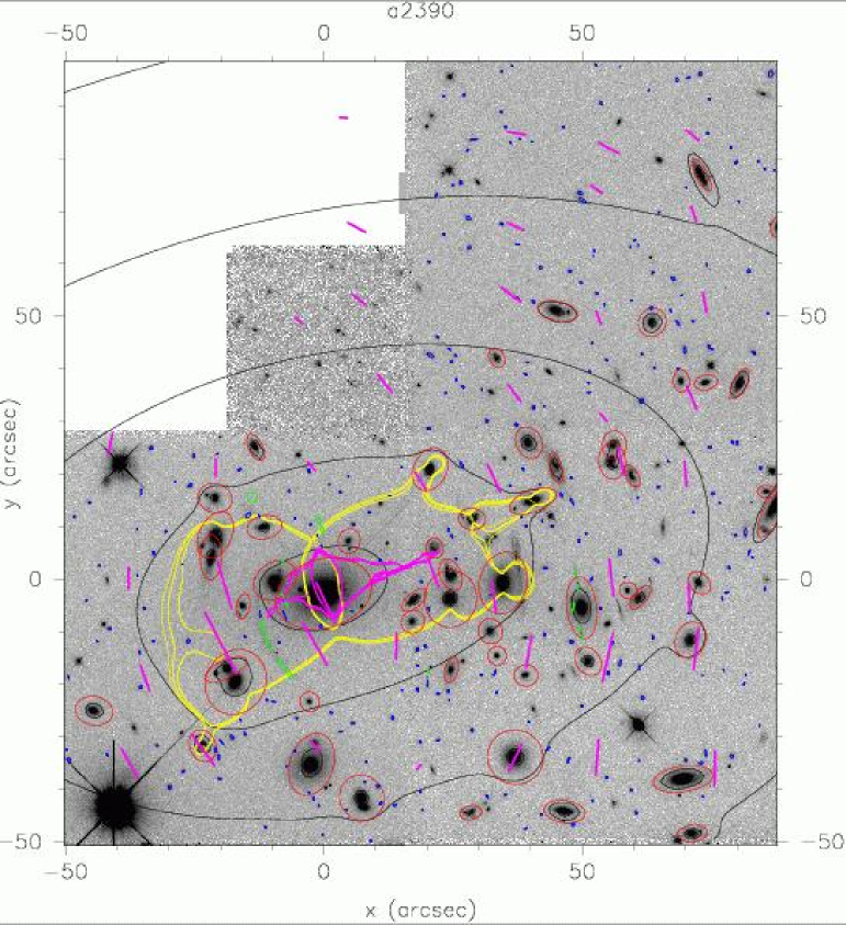
Figure 2: Mass model for A 2390: all included galaxy scale potentials are demarcated with ellipses and the critical curves computed for sources at $z=1,2\&3$ are also shown here for the best-fit mass model.

The most distant cluster in our sample is Cl 0054$-$27 at $z=0.57$. This is an optically-selected cluster with a dominant central galaxy (Couch et al. 1985). A multiply-imaged arc is visible in the HST images of this cluster with a measured a redshift of 3.2 for this feature (Leborgne, private communication). The X-ray luminosity of this cluster measured to be $2.5\,h^{2}\,10^{43}\,{\rm erg\,s^{-1}}$ in the 0.3 – 3.5 keV band, is lower than would be expected from the $L_{X}$ to the measured shear strength correlation for massive lensing clusters (see Fig. 2 of Smail et al. 1997 for the correlation between $L_{X}$ and $<g>$ for a sample of HST cluster-lenses). Smail et al. (1997) argue that this cluster is an example of a system that is elongated along the line-of-sight, leading to the low $L_{X}$ for the measured surface mass density. Obviously, in cases like this the mass estimate obtained from X-ray data which assumes spherical symmetry is unlikely to provide accurate results.

3.2 Lensing Constraints

There are two aspects to constructing a successful lens model for the clusters analyzed here. Firstly, we must identify multiply-imaged background sources with reliable redshift measurements whose properties can be used to constrain the total projected mass within the lens models. Secondly, we have to extend these models to larger radii using the coherent distortion signal induced in the shapes of faint, background galaxies by the foreground cluster potential well.

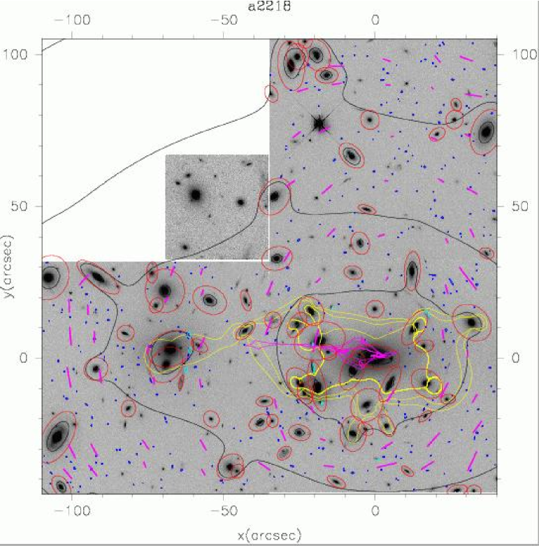
Figure 1: The best-fit mass model for A 2218. The confocal ellipses are the equi-potentials of the full potential including the substructure. The critical curves for the best-fit model computed for sources at $z=1,2\&3$ and caustics are also shown. The multiple images with measured redshifts that constrain the model are shown in cyan. All cluster members included in the mass modeling are marked with a red ellipse. The smoothed shear field is shown as pink sticks and the individual lensed galaxies are marked in blue. The critical lines and caustics are shown in yellow and pink respectively.

Both of these steps use the deep, high-resolution imaging provided for the cluster cores byHST. All five clusters analyzed here were observed with WFPC2 on-board HST for Guest Observer programs GO 5352 (A 2390 and Cl 2244$-$02), 5378 (Cl 0054$-$27) 5453 (Cl 0024+16) and 5701 (A 2218). The filters used for the observations were F555W ($V_{555}$) and F814W ($I_{814}$) or F702W ($R_{702}$). Observations of A 2218 were taken in the $R_{702}$ filter and all the other clusters studied here were observed in the $I_{814}$ filter. We have used the color information, when available, to test the identification of multiply-imaged sources in these fields. However, in the following analysis we use the reddest band available for a particular cluster to catalog objects and measure their shapes. The total exposure times are then 10.5 ks on both A 2390 and Cl 2244$-$02, 16.8 ks on Cl 0054$-$27 and 13.2 ks on Cl 0024+16, all in $I_{814}$, and 6.3 ks in $R_{702}$ on A 2218. The individual exposures were generally grouped in sets of four single-orbit exposures each offset by 2.0 arcsec to allow for hot pixel rejection. After standard pipeline reduction, the images were aligned using integer pixel shifts and combined into final frames using the iraf/stsdas task crrej. We retain the WFPC2 color system and hence use the zero points from Holtzman et al. (1995). The final images cover the central 0.8–1.6 Mpc of the clusters (Fig. 1–5) to a 5-$\sigma$ point-source limiting magnitude of $I_{814}\sim 26.0$ or $R_{702}\sim 26.5$–27.0 (Smail et al. 1997a).

Multiply-imaged background galaxies have been identified using HST imaging and spectroscopically confirmed in A 2218 by Kneib et al. (1996, 2004b), in A 2390 by Pello et al. (1999) and Frye & Broadhurst (1998), Cl 2244$-$02 (Smail et al. 1995a; Mellier et al. 1991), Cl 0024+16 by Broadhurst et al. (2000) and Cl 0054$-$27 by LeBorgne (priv. communication). These provide very strong constraints and drive the fit in the likelihood plane as we discuss below.

The second step in our analysis requires a statistical measure of the shear induced in the background field population. To achieve this we catalog faint objects in these frames and measure their shapes using the Sextractor image analysis package (Bertin & Arnouts 1995). Following Smail et al. (1997a, 1997b) we adopt a detection isophote equivalent to $\sim 1.3\sigma$ above the sky, where $\sigma$ is the standard deviation the sky noise, e.g. $\mu_{814}=25.0$ mag arcsec^-2 or $\mu_{702}=25.0$ mag arcsec^-2 for A 2218, and a minimum area after convolution with a 0.3 arcsec diameter top-hat filter of 0.12 arcsec². Analysis of our exposures provides catalogs of $\sim 800$ objects for each cluster across the 3 WFC chips. We discard the smaller, lower sensitivity, PC fields as well as a narrow border around each WFC frame in the following analysis. The imaging data (and catalogs) used here are identical to those previously analysed by Kneib et al. (1996) for A 2218, and Smail et al. (1997a, 1997b) for A 2218, Cl 0024+16 and Cl0054$-$27. In order to account for the error in shapes produced due to PSF, we adopt a method similar to that of Smith et al. (2004).

To constrain the weak lensing aspect of the models of the various clusters we must construct well-defined samples of background galaxies for which image parameters can be measured with adequate signal-to-noise. For simplicity in modeling we have adopted uniform magnitude limits across the sample. The faint magnitude limit is determined by the depth at which reliable images shapes can be measured in our shortest exposures. This is $R_{702}=26.0$, as set by the A 2218 exposure. The bright limit is set by our desire to reduce cluster galaxy contamination in the field samples for the most distant clusters and corresponds to a bright limit of $I_{814}=22.5$. When converting between the $R_{702}$ and $I_{814}$ limited samples, we have assumed a typical color for the faint field population at these depths of $(R_{702}\!-\!I_{814})\sim 0.5$ (Smail et al. 1995b). Hence our background galaxy cut is defined simply as $R_{702}=23$–26 or $I_{814}=22.5$–25.5. Cluster galaxies are chosen with an additional luminosity cut-off.

Applying these limits yields a typical surface density of $\sim 95$ field galaxies per arcmin², in good agreement with that measured in genuine ‘blank’ fields ($\sim 95\pm 10$ arcmin^-2) after correcting for differences in the photometric systems (Smail et al. 1995b). We thus estimate that any residual contamination in our catalogs from faint cluster members must be less than $\sim 5$–10%. The final sample size in a typical cluster, after applying both the magnitude and the area cuts (see Table 3), is $\sim 350-400$ galaxies.

To determine the contribution to the observed shear from systematic effects in the HST optics, detectors, or the reduction method, we have also modeled the PSF anisotropy using the methods adopted by Smith et al. (2004) and corrected the background image shapes accordingly.

3.3 Detailed mass models

A composite mass model is constructed for the clusters starting with the super-posed PIEMDs. The strong lensing data, i.e. the geometry, positions, relative brightness, redshifts and parities of the multiple images are used to obtain the mass enclosed within the Einstein radius which is used as an initial constraint for the integrated mass in the inner regions. The contribution to the shear and magnification from all potentials (large scale and small-scale perturbers) is calculated at the location of every observed background source galaxy and the inversion of the lensing equation is performed. The observed shape and magnification of each and every distorted background galaxy is compared to that computed from the model and the sub-halo mass distribution is modified iteratively till the best match between the observations and the model are found simultaneously for all background sources.

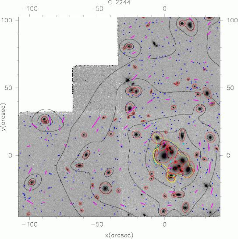
Figure 3: Mass model for Cl 2244.

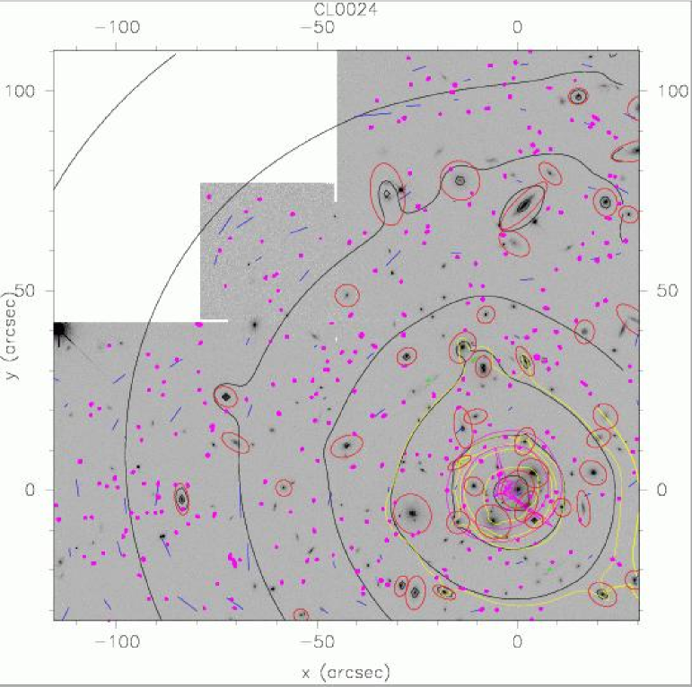
Figure 4: Mass model for Cl 0024+16. Note that this cluster has a smooth set of confocal equi-potentials. This model is in good agreement with the one recently published by Kneib et al. (2003) that extends out to 5 h^-1 Mpc.

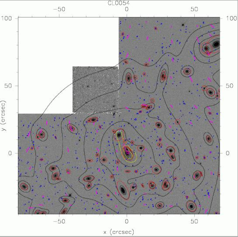
Figure 5: Mass model for Cl 0054$-$27. Although we require 2 smooth components in the inner most regions, the overall mass model for this cluster is a lot smoother compared to the others studied here.

The basic steps of our analysis involves the lens inversion, modeling and optimization, which are done using the lenstool software utilities (Kneib 1993). These utilities are used to perform the ray tracing from the image plane to the source plane with a specified intervening lens. This is achieved by solving the lens equation iteratively, taking into account the observed strong lensing features, positions, geometry and magnitudes of the multiple images. In some cases, we also include a constraint on the location of the critical line (between 2 mirror multiple images) to fasten the optimization. In Figs. 1–5, we show the iso-mass contours overlaid on their respective HST WFPC2 images. All the cluster galaxies included in the analysis have ellipses around them, and over-plotted are the critical curves (in yellow) for three different source redshifts ($z_{s}=1,2,3$), the multiple images (in cyan) and the smoothed background shear field (in magenta) for the best-fit model. Additionally, we fix the core radius of an $L^{*}$ sub-halo to be $0.1\,{\rm kpc}$, as by construction our analysis cannot constrain this quantity. In addition to the likelihood contours, the reduced $\chi^{2}$ for the best-fit model is also robust. We describe pertinent features of each cluster and their respective mass models below.

A2218

Our best fit mass model for the cluster is bimodal, composed of two large scale clumps around the cD and the second brightest cluster galaxy (Fig. 1 and Table 1). This model is an updated version of that constructed by Kneib et al. (1996). It includes 40 additional small-scale clumps that we associate with luminous early-type galaxies in the cluster core. Only about 10% of the total cluster mass is in the substructure i.e. associated with galaxy scale halos. The aperture mass, integrated over the truncation radius $r_{ap}\,=\,40$ kpc, yields a characteristic mass of $1.4\times 10^{12}\,M_{\odot}$, with a total mass-to light ratio in the V-band of $\sim\,5.8\pm 1.5$ and a central velocity dispersion of about $180\,{\rm km\,s}^{-1}$.

${z}$	$x$	$y$	$\epsilon$	${\theta}$	${\sigma}$	${r_{t}}$	${r_{c}}$
		arcsec	arcsec	deg	(km s-1)	(kpc)	(kpc)
A 2218
${0.17}$	${0.3}$	${1.4}$	${0.3}$	${-13}$	${1070}$	${900}$	${75}$
${0.17}$	${-67.5}$	${3.0}$	${0.2}$	${20}$	${400}$	${600}$	${25}$
A 2390
${0.23}$	${0.0}$	${0.0}$	${0.1}$	${17}$	${1100}$	${900}$	${55}$
${0.23}$	${-0.04}$	${-2.70}$	${0.4}$	${16}$	${450}$	${60}$	${10}$
Cl 2244$-$02
${0.33}$	${0.0}$	${0.0}$	${0.17}$	${45}$	${600}$	${900}$	${30}$
${0.33}$	${17.32}$	${-10.2}$	${0.1}$	${90}$	${300}$	${600}$	${20}$
Cl 0024+16
${0.39}$	${0.3}$	${1.4}$	${0.3}$	${-13}$	${1000}$	${900}$	${30}$
${0.39}$	${1.63}$	${71.3}$	${0.3}$	${45}$	${200}$	${200}$	${20}$
Cl 0054$-$27
${0.57}$	${0.0}$	${-1.0}$	${0.2}$	${-22}$	${1100}$	${900}$	${30}$

Table 1: Properties for the primary and (where relevant) secondary mass clumps in the clusters. The characteristic parameters are initially constrained by the positions, shapes and luminosities of the multiple-imaged objects and are then iteratively varied to match the weak shear field as well to obtain the optimal values (in the $\chi^{2}$ sense) in a likelihood scheme.

Additionally, we explore the relation between luminosity and mass (velocity dispersion, in fact) by allowing the index $\alpha$ to float. This is done by using an alternate choice of parameters to construct the likelihood function ${\cal L(\alpha,M_{\rm ap})}$. The results of this analysis are shown in Fig. 9. The retrieved value of the aperture mass $M_{\rm ap}$ is not particularly sensitive to the choice of $\alpha$.

A2390

The cluster has an unusual feature – a strongly lensed almost ‘straight arc’ (Pello et al. 1991) approximately 38 arcsec ($\sim$ 170 kpc) away from the central galaxy, in addition to many other arcs and arclets that have been utilized in our modeling. We find a best-fit mass model with two large-scale components (see Table 1 for their properties), that yield a projected mass within the radius defined by the brightest arc of $\sim 1.8\pm 0.2\times 10^{14}\,M_{\odot}$. Our best-fit composite lensing model for A 2390 incorporates 40 perturbers associated with early-type cluster members whose characteristic parameters are optimized in the maximum-likelihood analysis. We show the equi-potentials of this mass model overlaid on the HST WFPC2 data in Fig. 2, showing those cluster galaxies selected as perturbers and we also show the critical curves for three different source redshifts ($z_{s}=1,2,3$), the multiple images used to constrain the model and and the smoothed background shear field from the best-fit model. The integrated mass within the $\sim$ 18 kpc tidal radius for a typical $L^{*}$ cluster galaxy is about $6.4\times 10^{11}\,M_{\odot}$ giving a total mass-to-light ratio in the V-band of about $4.2\pm 1.3$. Once again 90% of the total mass of the cluster is consistent with being smoothly distributed.

Cl2244

This best-fit lens model for this cluster has two components but both have fairly low velocity dispersions (see Table 1). This is the least massive lensing cluster in the sample studied here. The X-ray mass estimate from the ASCA data Ota et al. (1998) is in good agreement with our best-fit lensing mass model. This is despite the fact that the X-ray temperature of Cl 2244$-$02 is at least a factor of two higher than that expected from the average luminosity-temperature relation.

The tidal truncation radius obtained for a typical $L^{*}$ cluster galaxy in Cl 2244 is the largest in the sample studied here and is $55\pm 12$ kpc. This is in consonance with the fact that the central density in Cl 2244 is the lowest. The total mass-to-light ratio in the V-band for a fiducial $L^{*}$ is $3.2\pm 1.2$. Approximately 20% of the total mass is in substructure within the mass range $10^{11}-10^{12.5}\,M_{\odot}$.

Cl0024

Our best fit mass model for the inner regions takes into account the small scale dark halos associated with the early-type members in the core, and requires a two component model for the sub-clusters (Table 1 and Fig. 4). Integrating the best-fit mass model shown in Fig. 4, we find that (i) about 10% of the total cluster mass is in galaxy-scale halos and (ii) the total mass estimate is in good agreement with that obtained by Kneib et al. (2003) where data from a much larger field of view was used.

Even on the large scales probed by Kneib et al. (2003) it was found that mass and light traced each other rather well at large radii. A typical $L^{*}$ cluster galaxy was found to have a truncation radius of $45\pm 5$ kpc, and a central velocity dispersion of $125\pm 7\,{\rm km\,s}^{-1}$.

Cl0054

The lensing signal from Cl 0054$-$27 is best fit by a single smooth dark matter component and sub-halos associated with bright, early-type members making it the only uni-modal cluster in the sample studied here. The mass enclosed within $\sim$ 400 kpc is of the order of $1.8\pm 0.4\times 10^{14}\,\odot$. The best-fit mass model is plotted in Fig. 5, with all the cluster galaxies included in the model shown explicitly.

The characteristic central velocity dispersion of a typical $L^{*}$ galaxy in this cluster is higher than in A 2218, A 2390 or Cl 0024+16, all of which are by contrast bimodal in the mass distribution. In this cluster about 20% of the total mass is in substructure. However, Cl 0054$-$27 is the most distant cluster studied here and is likely to be still evolving and assembling accounting for the high mass fraction in substructure.

Cluster	${z}$	${\rm N_{\rm cg}}$	${\rm N_{\rm bg}}$
A 2218	${0.17}$	${40}$	${358}$
A 2390	${0.23}$	${40}$	${378}$
Cl 2244-02	${0.33}$	${40}$	${398}$
Cl 0024+16	${0.39}$	${40}$	${344}$
Cl 0054-27	${0.57}$	${40}$	${426}$

Table 2: The number of background galaxies ${\rm N_{\rm bg}}$ and foreground lenses ${\rm N_{\rm cg}}$ for the clusters studied here. The number of background sources was determined usign a magnitude cut and the lenses were picked to be the 40 brightest, early-type galaxies from confirmed cluster members.

${\rm Cluster}$		${\sigma^{\ast}}$	${r_{t}^{\ast}}$	${M_{\rm ap}/L_{v}}$	$\rm{M^{\ast}}$	$\sigma_{\rm clus}$	${\rho_{\rm clus}(r=0)}$
		(km s-1)	(kpc)	(M⊙/L⊙)	(1011M⊙)	(km s-1)	(106 $M_{\odot}$ kpc-3)
A 2218	${0.17}$	${180\pm 10}$	${40\pm 12}$	${5.8\pm 1.5}$	$\sim\,14$	${1070\pm 70}$	3.95
A 2390	${0.23}$	${200\pm 15}$	${18\pm 5}$	${4.2\pm 1.3}$	$\sim\,6.4$	${1100\pm 80}$	16.95
AC 114	${0.31}$	${192\pm 35}$	${17\pm 5}$	${6.2\pm 1.4}$	$\sim\,4.9$	${950\pm 50}$	9.12
Cl 2244$-$02	${0.33}$	${110\pm 7}$	${55\pm 12}$	${3.2\pm 1.2}$	$\sim\,6.8$	${600\pm 80}$	3.52
Cl 0024+16	${0.39}$	${125\pm 7}$	${45\pm 5}$	${2.5\pm 1.2}$	$\sim\,6.3$	${1000\pm 70}$	3.63
Cl 0054$-$27	${0.57}$	${230\pm 18}$	${20\pm 7}$	${5.2\pm 1.4}$	$\sim\,9.4$	${1100\pm 100}$	15.84

As illustrated in Fig. 9, the derived mass is not a strong function of $\alpha$ given the errors. However, from other lensing work notably by McKay et al. (2001) and Wilson et al. (2001) it is clear that mass and light seem to trace each other rather tightly on galactic scales although in the inner-most regions of galaxies baryons appear to dominate density profiles. Note here that the choice of $\alpha$ determines only the scaling of the outer radius of a fiducial sub-halo with luminosity. With the data used in this paper it is not possible to distinguish between various values of $\alpha$ - some values are clearly more physical than others. Therefore, this implies that we are sensitive to the integrated mass within an aperture that is determined primarily by the anisotropy in the shear field and not on the details of the how the sub-halo masses are truncated. We also find that out to 500 kpc in all clusters only 10–20% of the total mass is associated with galaxy halos, at this radius (to which we are limited due to the size of the HST WFPC2 fields) most of the mass is in the large scale component. Needless this fraction is likely to be a strong function of cluster-centric radius. The dependence of the efficiency of tidal stripping with distance from the cluster can be explored with wide-field HST data and we are in the process of doing so for the cluster Cl 0024+16 (Natarajan et al. 2004).

4 Uncertainties

4.1 Systematic errors: robustness of the lens models

The following tests were performed for each cluster, (i) choosing random locations (instead of bright, early-type cluster member locations) for the perturbers; (ii) scrambling the shapes of background galaxies; (iii) choosing to associate the perturbers with the 40 faintest (as opposed to the 40 brightest) galaxies; (iv) randomly selecting known cluster galaxies as perturbers; (v) selecting late-type galaxies. None of the above cases (i)– (v) yields a convergent likelihood map, in fact all that is seen in the resultant 2-dimensional likelihood surfaces is noise.

The robustness of our results has been amply tested, however there are a couple of caveats that we ought to mention. As outlined above in this galaxy-galaxy lensing technique we are sensitive to only a restricted mass range in terms of secure detection of substructure. This is due to the fact that we are quantifying a differential signal above the average tangential shear induced by cluster, and we are inherently limited on average by the number of distorted background galaxies that lie within (1 - 2) tidal radii of cluster galaxies. This trade-off between requiring sufficient number of lensed background galaxies in the vicinity of the sub-halos and the optimal locations for the sub-halos leads us to choose the brightest 40 early-type cluster galaxies for each lens. With deeper, wider and more numerous images of clusters, expected in the future with a wide-field imager in space, such as the SNAP mission (Aldering et al. 2003) this technique can be pushed much further to probe down to lower masses in the mass function. It is possible that the bulk of the mass in sub-halos are in lower mass clumps (which in this analysis is essentially accounted for as part of the smooth component) and are in fact anti-correlated with positions of early-type galaxies.

Our results still hold true since we are filtering out only the most massive clumps via this technique. Note that one of the null tests performed above, associating galaxy halos with random positions in the cluster (and not on the locations of bright, early-type galaxies) resulted in pure noise. Even if we suppose that the bulk of the dark matter is associated with say, dwarf/very low surface brightness galaxies in clusters, then the spatial distribution of these galaxies is required to be fine-tuned such that these effects do not show up in the shear field in the inner regions implying that if at all they are likely to be more significant repositories of mass perhaps in the outskirts of clusters.

Guided by the current theoretical understanding of the assembly of clusters, dwarf galaxies are unlikely to survive in the high density core regions of galaxy clusters studied here. When studies such as presented here are applied on a larger scales to distances over a few Mpc’s from the cluster center (analysis of the mosaic-ed HST images as in Natarajan et al. 2004) we can explore further the relation between mass and light, and the variation of tidal truncation radii with distance from the cluster center.

4.2 Random errors

The principal sources of error in the above analysis are (i) shot noise – we are inherently limited by the finite number of sources sampled within a few tidal radii of each cluster galaxy; (ii) the spread in the intrinsic ellipticity distribution of the source population; (iii) observational errors arising from uncertainties in the measurement of ellipticities from the images for the faintest objects and (iv) contamination by foreground galaxies mistaken as background. As mentioned in Section 2.2.2, the partitioning of mass into sub-halos and the smooth component as done here is largely independent of the $N(z)$ of background galaxies.

In terms of the total contribution to the error budget, performing simulations we find that the shot noise is the most significant source of error $\sim 50\%$; followed by the width of the intrinsic ellipticity distribution which contributes $\sim 20\%$, and the other three sources together contribute $\sim 30\%$. This elucidates the future strategy for such analyses - going significantly deeper and wider in terms of the field of view is likely to provide considerable gains. Mosaic-ed ACS images are the ideal data sets for this galaxy-galaxy lensing analyses, and such work is currently in progress.

5 Results

We successfully construct high resolution mass models for all five clusters from the unambiguous galaxy-galaxy lensing signal detected using the maximum-likelihood analysis. We also detect a cut-off in the extent of a fiducial halo, which we argue is a result of tidal stripping of cluster galaxies that traverse through the central regions of the cluster. All our lens models are plotted in Figs. 1–5. The maximum-likelihood analysis yields the following: (i) the mass-to-light ratio in the $V$-band of a typical L^∗ does not evolve significantly as a function of redshift, (ii) the fiducial truncation radius of an $L^{*}$ varies from about 15 kpc at $z=0.18$ to 70 kpc at $z=0.57$, (iii) the typical central velocity dispersion is roughly 180  km s^-1.

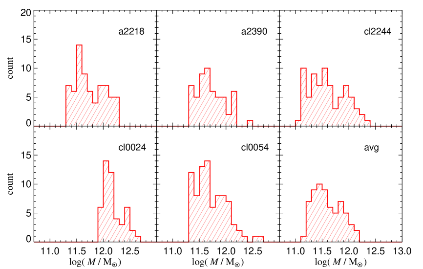
Figure 8: Sub-halo mass spectrum retrieved from the maximum-likelihood analysis for the five HST cluster-lenses studied here.

We present the luminosity function of early-type confirmed cluster members chosen as perturbers in all 5 clusters in Fig. 7. For the galaxy model (PIEMD) adopted in our analysis, the total mass of an L^∗ varies with redshift from $\sim 2.8\times 10^{11}\,M_{\odot}$ to $\sim 7.7\times 10^{11}\,M_{\odot}$ The mass-to-light ratios quoted here take passive evolution of elliptical galaxies into account as given by the stellar population synthesis models of Bruzual & Charlot (2003), therefore any detected trend reflects pure mass evolution (see Table 2 and Fig. 6). The mass obtained for a typical bright cluster galaxy by Tyson et al. (1998) using only strong lensing constraints inside the Einstein radius of the cluster Cl 0024+1654, at $z=0.41$, is consistent with our results. All error bars quoted here are $\sim 3\sigma$. Scaling laws were needed to relate the mass to the light (see eqn. 30), the effect of the assumed form on the derived fiducial sub-halo mass of an $L^{*}$ is show in Fig. 8.

By construction, the maximum-likelihood technique presented here provides the mass spectrum of sub-halos in the cluster directly (see Fig. 8). Note that as stated before in performing the likelihood analysis to obtain characteristic parameters for the sub-halos in the cluster it is assumed that light traces mass. This is an assumption that is well supported by galaxy-galaxy lensing studies in the field (Wilson et al. 2001) as well as in clusters (Clowe & Schneider 2002). In fact, all lens modeling and rotation curve measurements suggest an excess of baryons in the inner regions. Note however that for our choice of mass model (the PIEMD) the mass to light ratio is not constant with radius within an individual galaxy halo. Since the procedure involves a scaled, self-similar mass model that is parametric, we obtain a mass estimate for the dark halos (sub-halos) as a function of their luminosity. This provides us with a clump mass spectrum. Tidal truncation by the cluster causes these galaxy halo masses to be lower than that of equivalent luminosity field galaxies at comparable redshifts obtained from galaxy-galaxy lensing. The fraction of mass in these clumps is only 10–20% of the total mass of the cluster within the inner $500\,h^{-1}\,{\rm kpc}$ of these high central density clusters. The remaining 80–90% of the cluster mass is consistent with being smoothly distributed (in clumps with mass $M\,<\,10^{10}\,M_{\odot}$), the precise composition of this component depends on the hitherto unknown nature of dark matter. Note that the the upper and lower limits on the mass spectrum vary from cluster to cluster due to the difference in the luminosity functions of cluster galaxies. These mass functions can now be directly compared to the sub-halo mass functions of dark matter halos in cosmological N-body simulations, the results of which are presented elsewhere (Natarajan & Springel 2004).

6 Conclusions and Discussion

In this paper, we present (i) high resolution mass models for lensing clusters and (ii) the mass function of sub-halos inside these clusters. Detailed results of the application of our galaxy-galaxy lensing analysis techniques to five HST cluster lenses (as well as a further cluster we have previously analyzed in an identical manner) are used to construct high resolution mass models of the inner regions. In order to do so we have utilized both strong and weak lensing observations for these massive clusters. The goal is to quantify substructure in the cluster assuming that the sub-halos follow the distribution of bright, early-type cluster galaxies. Similar attempts have been made in the lower density field environment yielding typical galaxy masses and central velocity dispersions. The mass distribution for a typical galaxy halo inferred from field studies are extended with no discernible cut-off. By contrast in the cluster environments probed in this work we detect an edge to the mass distribution in cluster galaxies. We have performed various stringent checks to ascertain that this is not an artifact of the choice of mass model and rather evidence for tidal stripping by the global cluster potential well. Aside from the detailed lens models, we also present the first ever mass spectrum (albeit within a limited mass range with sub-halo masses ranging from $10^{11}-10^{12.5}\,M_{\odot}$) of substructure in the inner regions of these clusters. The survival and evolution of substructure offers a stringent test of structure formation models within the CDM paradigm. Sub-halos of the scale detected in all these clusters indicate a high probability of galaxy–galaxy collisions over a Hubble time within a rich cluster. However, since the internal velocity dispersions of these clumps associated with early-type cluster galaxies ($\sim 150$–250 km s^-1) are much smaller than their orbital velocities, these interactions are unlikely to lead to mergers, suggesting that the encounters of the kind simulated in the galaxy harassment picture by Moore et al. (1996) are the most frequent and likely. High resolution cosmological N-body simulations of cluster formation and evolution (De Lucia et al. 2004; Ghigna et al. 1998; Moore et al. 1996), find that the dominant interactions are between the global cluster tidal field and individual galaxies after $z=2$. The cluster tidal field significantly tidally strips galaxy halos in the inner 0.5 Mpc and the radial extent of the surviving halos is a strong function of their distance from the cluster center. Much of this modification is found to occur between $z=0.5$–0. The trends seen in halo size $r_{t}^{*}$ with redshift detected in our analysis of these clusters (Natarajan et al. 2002a) are broadly in agreement with high-resolution cosmological N-body simulations of currently popular cosmological models (De Lucia et al. 2004). Further interpretation and comparison of these results with theoretical models and high resolution N-body simulations is presented elsewhere (Natarajan & Springel 2004).

Figure 6: The results of the maximum likelihood analysis. Top left panel: the variation of the mass-to-light ratio in the V-band as a function of redshift for a typical $L^{*}$ sub-halo; Top right panel: the central velocity dispersion of a typical $L^{*}$ sub-halo in the cluster versus the velocity dispersion of the cluster; Bottom left panel: the central velocity dispersion versus the tidal radius of an $L^{*}$ sub-halo which is the result of the maximum likelihood analysis; Bottom right panel: the tidal truncation radius versus central density of the cluster.

Figure 7: Luminosity function of the selected early-type galaxies. For four clusters (A 2218, AC114, Cl 0024+16, and Cl 0054-27) morphological classification and membership information was obtained from the MORPHS collaboration. For A 2390 and Cl 2244-02 a magnitude cut was used to delineate cluster members.

Figure 9: The retrieved mass $M_{\rm ap}$ for an $L^{*}$ cluster galaxy in A2218 as a function of the choice of the scaling parameter $\alpha$ that tunes the outer edge of the mass distribution used to model the sub-halos.

References

- (1)
- (2) Aldering, G., et al., 2003, SPIE 4835, 40 (astro-ph/0209550)
- (3)
- (4) Barger, A. J., et al., 1998, ApJ, 501, 522
- (5)
- (6) Binney, J., & Tremaine, S., 1987, Galactic Dynamics, (Princeton: Princeton U. Press), Ch. 7
- (7)
- (8) Brainerd, T., Blandford, R., & Smail, I., 1996, ApJ, 466, 623
- (9)
- (10) Brainerd, T., & Specian, M., 2003, ApJ, 593, L7
- (11)
- (12) Bruzual, G., & Charlot, S., 2003, MNRAS, 344, 1000
- (13)
- (14) Couch, W.J., Barger, A.J., Smail, I., Ellis, R.S., Sharples, R.M., 1998, ApJ, 497, 188
- (15)
- (16) Couch, W.J., Shanks, T., & Pence, W.D., 1985, MNRAS, 213, 215
- (17)
- (18) Danese, L., de Zotti, G., & di Tullio, G. 1980, ApJ, 82, 322
- (19)
- (20) Dave, R., Spergel, D., Steinhardt, P. J., & Wandelt, B. 2001, ApJ, 547, 574
- (21)
- (22) Dell’ Antonio, I., & Tyson, J. A. 1996, ApJ, 473, L17.
- (23)
- (24) Fischer, P., et al. 2000, AJ, 120, 1198
- (25)
- (26) Furlanetto, S., & Loeb, A. 2002, ApJ, 565, 854
- (27)
- (28) De Lucia, G., et al., 2004, MNRAS, 348, 333
- (29)
- (30) Ebbels, T. M. D. et al., 2000, private communication.
- (31)
- (32) Ghigna, S., Moore, B., Governato, F., Lake, G., Quinn, T., & Stadel, J., 1998, MNRAS, 300, 146
- (33)
- (34) Girardi, M., et al. 1997, ApJ, 490, 56
- (35)
- (36) Gnedin, O., & Ostriker, J. P. 2001, ApJ, 561, 61
- (37)
- (38) Griffiths, R. E., Casertano, S., Om, M., & Ratnatunga, K. U. 1996, MNRAS, 282, 1159
- (39)
- (40) Kassiola, A., & Kovner, I. 1993, ApJ, 417, 474
- (41)
- (42) Kneib, J-P., Ellis, R. S., Couch, W., Smail, I. R., & Sharples, R. 1996, 471, 643
- (43)
- (44) Kneib, J-P., et al., 2003, ApJ, 598, 804
- (45)
- (46) Hoekstra, H., Yee, H. K., & Gladders, M., 2004, ApJ, 606, 67
- (47)
- (48) Hudson, M. J., Gwyn, S. D. J., Dahle, H., & Kaiser, N., 1998, ApJ, 503, 531
- (49)
- (50) Le Borgne, J-F., Pello, R., & Sanahuja, B. 1992, A&AS, 95, 87
- (51)
- (52) Le Fevre, O., et al., 2004, A&A, 417, L839
- (53)
- (54) McKay, T. et al. 2002, ApJ, 571, L85
- (55)
- (56) Miralda-Escude, J. 2002, ApJ, 564, 1019
- (57)
- (58) Moore, B., Katz, N., Lake, G., Dressler, A., & Oemler, A. 1996, Nature, 379, 613
- (59)
- (60) Natarajan, P., & Kneib, J-P. 1996, MNRAS, 283, 1031
- (61)
- (62) Natarajan, P., & Kneib, J-P. 1997, MNRAS, 287, 833
- (63)
- (64) Natarajan, P., Kneib, J-P., Smail, I., & Ellis, R. S. 1998, ApJ, 499, 600 [NKSE98]
- (65)
- (66) Natarajan, P., Kneib, J-P., & Smail, I., 2002a, ApJ, 580, L11
- (67)
- (68) Natarajan, P., Loeb, A., Kneib, J-P., & Smail, I., 2002b, ApJ, 580, L17
- (69)
- (70) Natarajan, P., & Springel, V., 2004, ApJ Lett., in press
- (71)
- (72) Natarajan et al., 2004, in preparation
- (73)
- (74) Rakos, K., Dominis, D., & Steindling, S. 2000, A&A, 369,750
- (75)
- (76) Smail, I., et al., 1995b, ApJ, 449, L105
- (77)
- (78) Smail, I., Dressler, A., Couch, W.J., Ellis, R.S., Oemler, A., Butcher, H., Sharples, R.M., 1997a, ApJS, 110, 213
- (79)
- (80) Smail, I., et al., 1997b, ApJ, 479, 70
- (81)
- (82) Smail, I., et al. 2001, MNRAS, 323, 839
- (83)
- (84) Spergel, D., & Steinhardt, P. J. 2000, Phys. Rev. Lett., 84, 17, 3760
- (85)
- (86) Springel, V., et al, 2001, MNRAS, 328, 726
- (87)
- (88) Stoehr, F., et al. 2002, MNRAS, 335, L84
- (89)
- (90) Taylor, J. E., & Babul, A. 2001, ApJ, 559, 716
- (91)
- (92) Tyson, J. A., Kochanski, G., & De’ll Antonio, I. P., 1998, ApJ, 498, L107
- (93)
- (94) van Dokkum, P., Franx, M., Kelson, D., & Illingworth, G.,1998, ApJ, 504, L-17
- (95)
- (96) Wolf, C., et al., 2004, A&A, 421, 913
- (97)
- (98) Wilson, G., Kaiser, N., Luppino, G. A., & Cowie, L. L. 2001, ApJ, 555, 572
- (99)
- (100) Yoshida, N., Springel, V., White, S. D. M., & Tormen, G. 2000, ApJ, 535, L103
- (101)