3D-simulation of the Outer Convection-zone of an A-star

Abstract

The convection code of Nordlund & Stein has been used to evaluate the 3D, radiation-coupled convection in a stellar atmosphere with $T_{\rm eff}=7300$ K, log$g=4.3$ and [Fe/H]$=0.0$, corresponding to a main-sequence A9-star. I will present preliminary comparisons between the 3D-simulation and a conventional 1D stellar structure calculation, and elaborate on the consequences of the differences.

1 Introduction

From 3 dimensional simulations of convection, it has been known for the last two decades that convection grows stronger with increasing effective temperature and decreasing gravity. By stronger, is here meant larger Mach-numbers, larger turbulent- to total-pressure ratios and larger convective fluctuations in temperature and density. The stronger convection has also been accompanied by increasing departures from 1D stellar models that fail to predict the extensive overshoot into the high atmosphere, the turbulent pressure and its effect on the hydrostatic equilibrium, the temperature fluctuations and the coupling with the highly non-linear opacity. The latter has the effect of heating the layers below the photosphere, thereby expanding the atmosphere, as also done by the turbulent pressure. The various 1D convection theories/formulations, e.g., classical mixing-length (Böhm-Vitense, 1958), non-local extensions to it (Gough, 1977) or an independent formulation based on turbulence (Canuto & Mazzitelli, 1992), all have similar shortcomings with respect to the simulations. Their predictive power is further limited by the free parameters involved.

Going towards earlier type stars, apart from stronger convection, also means a more shallow outer convection zone. This combination is rather unpredictable and is the main motivation for the work presented here. Classical predictions call for the outer convection zone to disappear close to the transition between A and F stars, but details about where and how this transition occurs can only be gained from realistic, 3D simulations, as outlined below.

2 The simulations

The simulation presented here was carried out using the code of Nordlund & Stein (1990) and is further described in Nordlund (1982), Stein (1989) and Stein & Nordlund (2003).

The basis of hydrodynamics is the Navier-Stokes equations, and the code employs the conservative or divergence form

$$\frac{\partial\varrho}{\partial t} = -\nabla\cdot(\varrho\hbox{\mib u})$$ (1)

$${\partial\varrho\hbox{\mib u}\over\partial t} = -\nabla\cdot(\varrho\hbox{\mib u}\hbox{\mib u})-\nabla P_{\rm g}+\varrho\hbox{\mib g}$$ (2)

$$\frac{\partial\varrho\varepsilon}{\partial t} = -\nabla\cdot(\varrho\varepsilon\hbox{\mib u})-P_{\rm g}\nabla\cdot\hbox{\mib u}+\varrho(Q_{\rm rad}+Q_{\rm visc})\ ,$$ (3)

where $\varrho$ is the density, $P_{\rm g}$ is the gas pressure, $\varepsilon$ is the specific internal energy, u is the velocity field, g is the gravitational acceleration and $Q_{\rm rad}$ and $Q_{\rm visc}$ are the radiative and viscous heating, respectively, the latter arising from the numerical diffusion applied.

Equations (1)–(3) describe the conservation of mass, momentum and energy, respectively, with sources and sinks on the right-hand-side. For the convection code the equations are preconditioned, by dividing by $\varrho$, to improve handling of the large density contrast between the top and bottom of the simulations.

The vertical component of the momentum equation, Eq. (2), can be written

$$F_{z}=-\frac{\partial(\varrho u_{z}^{2}+P_{\rm g})}{\partial z}+\varrho g\ ,$$ (4)

as we have chosen g to be in the $z$-direction. With $F_{z}=0$ this equation describes hydrostatic equilibrium, where the gas pressure and the turbulent pressure, $P_{\rm turb}=\varrho u_{z}^{2}$, provide support against gravity.

The gas pressure, $P_{\rm g}(\varrho,\varepsilon)$, and the opacities going into the computation of the radiative heating, $Q_{\rm rad}$, form the atomic physics basis for the simulations. The continuous opacities are calculated from the MARCS-package (Gustafsson, 1973) and subsequent updates as detailed in Trampedach (1997), the line opacity is in the form of opacity distribution functions (ODFs) (Kurucz, 1992), and the equation of state accounts explicitly for all ionization stages of the 15 most abundant elements (Hummer & Mihalas, 1988; Däppen et al., 1988).

The present simulation is performed on a $100\times 100\times 82$-point grid, has $T_{\rm eff}=7300$ K, log$g=4.3$ and [Fe/H]$=0.0$, and therefore corresponds to a A9 dwarf on the main-sequence. The computational domain is 11.5 Mm on each side, and 13.1 Mm deep, of which 1.5 Mm is above the photosphere.

So far the convection code has only been used for stars that were convective at the bottom boundary, so in order to accommodate this simulation, the boundary condition was changed and evaluation of radiative heating in optically thick layers was included.

The simulation was carried out in the plane-parallel approximation and includes no rotation or magnetic fields, and has a simple Solar abundance (Anders & Grevesse, 1989). Both thermodynamics and radiative transfer is performed in strict LTE. The velocity-field is too large, through-out the simulation domain, to support segregation of elements, rendering diffusion and radiative levitation of individual species, comfortably irrelevant.

3 Comparison with 1D models

In Fig. 1 the temporal and horizontal average of the simulation is compared with a corresponding 1D stellar model. From the solid black curve in panel a) we see that this simulation has an impressive turbulent pressure, making up almost 35% of the total pressure about 700 km below the photosphere (it is about 13% in Solar simulations). The mach-numbers reaching Mach 0.7 as shown with the dashed black line, is equally impressive. The convection is much less efficient compared to the Solar case, and invokes both higher velocities, as seen in panel a), and higher super-adiabatic gradient, as seen from the black curve in Panel b) of Fig. 1. The two gray curves show the $P_{\rm turb}/P_{\rm tot}$-ratio and $\nabla-\nabla_{\rm ad}$ for two 1D envelope models using the standard mixing-length formulation of convection (Böhm-Vitense, 1958). The solid line is for $\alpha=1.0$ and the dashed line for $\alpha=2.0$, in an attempt to bracket the behavior of the simulation. One glance at Fig. 1 makes it clear that no mixing-length model can reproduce the outer few percent of an A9 dwarf. The convection zone extends further up into the atmosphere and has much broader features than possible with mixing-length models. We also see that overshoot from the convection zone supports an appreciable velocity-field, with velocities of 2–3 km s^-1, and obvious consequences for spectral line shapes.

The large $P_{\rm turb}$ results in smaller temperatures at the same hydrostatic pressure, when compared to a 1D model. This can be translated into higher pressures and densities on an optical depth scale. Consequently the derived population of line-producing states in atoms, ions and molecules will be misleading and result in erroneous abundance analysis.

The mismatch between the simulation and the 1D models in the atmosphere is actually so profound that no mixing-length model with $T_{\rm eff}$ and $g_{\rm surf}$, consistent with the simulation, can be found to match the simulation (i.e., $P$, $\varrho$ and $T$) at the bottom. This means that stellar structure and evolution calculations are misplaced in the HR-diagram, with implications for age-determinations of globular clusters and our general knowledge of the interior and evolution of A-stars.

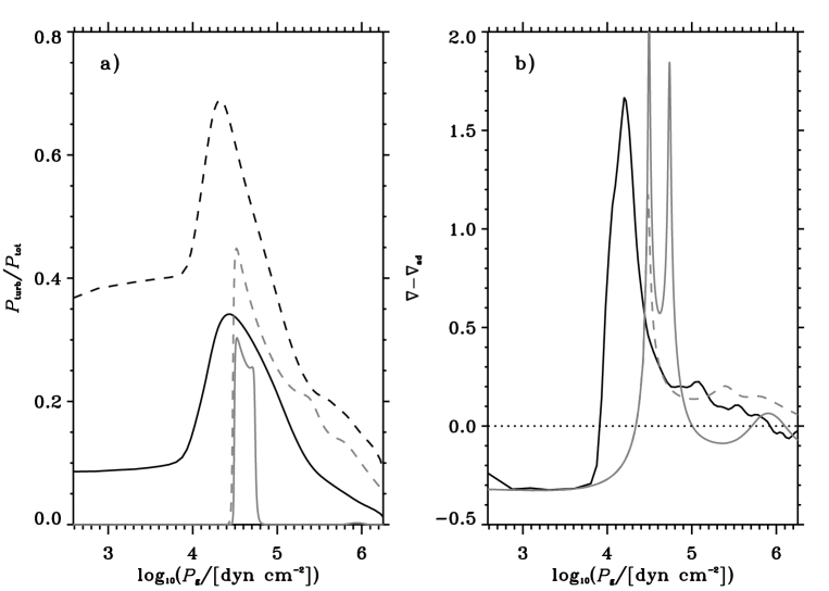
Figure 1: Comparisons between the simulation and two 1D, mixing-length models. In both panels the black solid line shows the temporal- and horizontally averaged simulation, and the gray solid line shows the same quantity for a 1D model with $\alpha=1.0$ and the dashed gray curve is for $\alpha=2.0$. Panel a) shows the turbulent- to total-pressure ratios, and the dashed black line shows the RMS Mach-numbers. Panel b) shows the super-adiabatic gradient, with the dotted zero-line aiding the location of the borders of the convection zones.

4 Temperature inversion

This simulation, which is the hottest performed with this code, displays some large and persistent temperature inversions, 1.5-2.5 Mm below the photosphere. They have an amplitude of up to 8 000 K and are about 0.5 Mm deep. During the meeting, Noels suggested that there might be a correlation between the turbulent pressure and the low temperatures; keeping $P_{\rm tot}$ and $\varrho$ constant to ensure hydrostatic equilibrium, a large $P_{\rm turb}$ would force a low temperature. This is, however not observed in the simulations. There is no correlation between the temperature inversion and $P_{\rm turb}$ – nor are there correlations with vertical or horizontal velocities, or the density contrast. There is, however, a strong correlation with the vertical force (see Eq. 4), as the force on the plasma in the temperature inversion is always outwards (the $-z$-direction). Furthermore, the vorticity is clearly skewed towards larger values in the inversion layer, especially when compared to the upflow, but also with respect to the down-drafts.

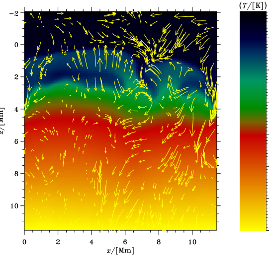
Figure 2: A vertical slice of a snapshot showing a temperature inversion. The color-scale shows temperature, and the arrows indicate the velocity-field.

Fig. 2 shows a vertical snapshot in temperature, displaying a typical temperature inversion. The arrows indicate the velocity field, with the maximum length corresponding to 2.9 km s^-1. The temperature inversion extends some 6 Mm across the left side of the plot, at a height of 2 Mm. It is connected to the downdraft at the edge, but it never connects with the downdraft to the right of the center. The velocity field there is connected, though, but the colder plasma from the inversion is compressed on the way to the downdraft, and therefore heated. The velocity field is diverging in the $z$-direction, neutral in the $x$-direction and convergent in the $y$-direction, perpendicular to the plane of the figure – the net-flow is convergent. The features observed in this simulation are cylindrical in the horizontal direction, with width and depth being similar and the length being 5–10 times larger.

The temperature inversions seem to develop when the local photosphere has subsided to about 2 Mm below the average photosphere, at the edge of a granule. The layers above, closer to the height of the average photosphere, then heats up, leaving a cooler area in between – the temperature inversion. In white-light surface intensity, this now looks like the edge of a normal granule. The inversion immediately starts eroding from the newly heated region on top moving down, and presumably from heating by the surroundings. The temperature profile after this sequence, looks like that of a downdraft, and from the surface, what looked like the edge of a normal granule, collapse as the temperature inversion below disappear. The whole cycle takes about 5 min.

The reason for this behavior is still under investigation, but it might be connected to the local minimum in $\nabla_{s}$, as seen in Fig. 1 around $\log_{10}P_{\rm g}\simeq 4.9$ corresponding to $z\simeq 1.9$ Mm.

5 Summary

A realistic 3D simulation of convection in the surface layers of a A9 dwarf reveals profound differences between that and a conventional 1D stellar structure model, as indicated in Sect. 3. In general, the simulations have much smoother and broader convection-zone features, compared to mixing-length models.

We are also treated to a new phenomena, as the simulations display repeated local temperature inversions just below the photosphere (cf., Sect. 4). The mechanism responsible for these large inversions, have not been uncovered yet, but it being an effect of large fluctuations in the turbulent pressure, has been ruled out.

This is still work in progress, and in the future, this and other simulations will be used for evaluation of spectral lines, limb-darkening, broad-band colors, granulation-spectra and p-mode spectra.

CowleyDid you get a higher contrast between hot and cold regions than in simulations of cooler stars? At one time I though the ionization imbalance that we observe in some cool Ap stars might be explained by such temperature inhomogeneities. But I did some test calculations and found this could not explain the ionization – at least not with the numerical models I had. TrampedachThe RMS temperature fluctuations at $\tau=1$ on a Rosseland optical depth scale, are about twice as large for the A9 simulation ($\sim 610$ K) as for the Solar simulation ($\sim 300$ K). For the latter, the RMS fluctuations stay below 750 K, peaking at $\tau=10$, whereas in the A9 simulation they grow almost exponentially to reach 5000 K at $\tau=100$.

I don’t know what kind of numerical models you have used, but a decisive factor in the emergent spectra from the convection simulations is the asymmetry of the distributions of temperatures, densities and velocities, as well as their correlations. These characteristics are hard to predict without realistic simulations.

PiskunovWhat is the height of the temperature inversion and the filling factor of the effect? Do you see significant changes of the filling factor? TrampedachThe temperature inversions are about 0.5–1.0 Mm deep and peak at a depths of 1.5–2.5 Mm. They involves from 2% to 8% of the horizontal area, with an average of about 5%.

NoelsDo you find a high turbulent pressure in the region of temperature inversion? If so, I would suggest to investigate this point in relation to the origin of the temperature inversion. TrampedachThere is no obvious correlation between the temperature inversion and the local turbulent pressure. I would refer to Sect. 4 for the present extent of my analysis.

GrevesseMicro-turbulence and macro-turbulence needed with 1D stellar photosphere models are not needed anymore with 3D models. Why is it not the same when 3D models are used, instead of 1D models, for A stars? TrampedachI don’t think that has changed, going from solar-like stars, to A stars. I think what you are alluding to, is the lack of reversal of bisector shape in the A star simulations presented by Freytag (elsewhere in these proceedings). I don’t know the reason for this and the only major thing missing from those simulations is line-blanketing. Whether that will make the difference is unclear and will have to await further simulations. It is important to understand that theoretical bisectors from 1D models are straight, no matter how much micro- or macro-turbulence is applied. The shape of bisectors is a higher order problem, that cannot be addressed with 1D models.

References

- Anders & Grevesse (1989) Anders, E., Grevesse, N. 1989, Geochim. Cosmochim. Acta 53(1), 197
- Böhm-Vitense (1958) Böhm-Vitense, E. 1958, Zs. f. Astroph. 46, 108
- Canuto & Mazzitelli (1992) Canuto, V. M., Mazzitelli, I. 1992, ApJ 389, 724
- Däppen et al. (1988) Däppen, W., Mihalas, D., Hummer, D. G., Mihalas, B. W. 1988, ApJ 332, 261
- Gough (1977) Gough, D. O. 1977, ApJ 214, 196
- Gustafsson (1973) Gustafsson, B. 1973, Upps. Astr. Obs. Ann. 5(6)
- Hummer & Mihalas (1988) Hummer, D. G., Mihalas, D. 1988, ApJ 331, 794
- Kurucz (1992) Kurucz, R. L. 1992, Rev. Mex. Astron. Astrofis. 23, 45
- Nordlund (1982) Nordlund, Å. 1982, A&A 107, 1
- Nordlund & Stein (1990) Nordlund, Å., Stein, R. F. 1990, Comput. Phys. Commun. 59, 119
- Stein (1989) Stein, R. F. 1989. In: R. J. Rutten, R. J. and G. Severino, G. (eds.), “Solar and stellar granulation”, Kluwer Academic Publishers, 381
- Stein & Nordlund (2003) Stein, R. F., Nordlund, Å. 2003. In: I. Hubeny, I., D. Mihalas, D., and K. Werner, K. (eds.), “Stellar atmosphere modeling”, Vol. 288 of Conf. Ser., ASP, ASP, San Francisco, 519
- Trampedach (1997) Trampedach, R. 1997. Master’s thesis, Aarhus University, Århus, Denmark