Observational constraints on generalized Chaplygin gas model

Abstract

The generalized Chaplygin gas model with parameter space $\alpha>-1$ is studied in this paper. Some reasonable physical constraints are added to justify the use of the larger parameter space. The Type Ia supernova data and age data of some clusters are then used to fit the model. We find that the parameters have bimodal distributions. For the generalized Chaplygin gas model, we also find that less free parameters fit the data better. The best fit model is the spatially flat model with baryons. The best fit parameters are: $\Omega_{m0}=0.044$, $w_{c0}=-0.881$ and $\alpha=1.57$. The transition redshift is $z_{T}=0.395$.

I Introduction

The mounting evidences suggest that the Universe is expanding with acceleration sp99 ; agr04 ; wmap . This reveals that the Universe is dominated by dark energy with negative pressure, whose energy density fraction is about 2/3 at present. The nature and origin of dark energy is still mysterious, leaving theoretic physicts searching for novel answers. Althoug a cosmological constant may be responsible for the accelerating expansion of the Universe and be consistent with current observational data, the extremely smallness of the value of the cosmological constant brings a big challenge to us. It is also possible that the mechanism at work is dynamical. A dynnamical candidate to provide dark energy may be supplied by a slowly rolling scalar field, widely referred as “quintessence field” quint . There are also models of a scalar field with non-canonical kinetic term, known as “k-essence” kessence or “tachyonic” models tachyon . Other alternative dark energy models include the holographic dark energy model holo and the extra-dimensional motivated models dgp .

Among the cosmological community, the consensus about our Universe is the so called “concondance model”: 95% percent of the Universe is composed of dark components. Recently the Chaplygin gas model with exotic equation of state $p=-A/\rho$ was proposed to explain both dark enrgy and dark matter chap . The Chaplygin gas model was later generalzied to the generalized Chaplygin gas (GCG) model with equation of state $p_{c}=-A/\rho_{c}^{\alpha}$ gcg . The novel feature of this model is that it unifies dark energy and dark matter in one model. Sandvik and coauthors claimed that the matter power spectrum essentially ruled the GCG model out sandvik . However, their analysis does not include the effect of the baryons. Beça and collabrators showed that it is important to include baryons in the study of large scale structure and the conclusion changed when baryons were included beca . It should also be noted that the results in sandvik was based on linear theory of perurbations and neglected any non-linear effects.

The GCG model has been extensively studied in the literature gcg1 ; gcg2 . The GCG model was also studied in the framework of modified Friedman equation in gcgmfe . In this paper, we consider both dust like matter and GCG as the source. The dust like matter may be just baryons or a portion of dark matter. Unlike other studies, we allow the parameter $w_{c0}=-A_{s}$ to be less than $-1$ and the parameter $\alpha$ to be in the region $-1<\alpha<0$ in addition to the usual region $\alpha>0$. Some physically reasonable conditions are then applied to the model to constrain the parameters. Therefore, the model considered here is more general in addition to be physical.

II GCG model

In a homogeneous and isotropic universe, the Friedmann-Robertson-Walker (FRW) space-time metric is

$$ds^{2}=-dt^{2}+a^{2}(t)\left[{dr^{2}\over 1-k\,r^{2}}+r^{2}\,d\Omega\right].$$ (1)

For a null geodesic, we have

$$\int_{t_{1}}^{t_{0}}{dt\over a(t)}=\int_{0}^{r_{1}}{dr\over\sqrt{1-kr^{2}}}\equiv f(r_{1}),$$ (2)

where

$$f(r_{1})=\left\{\begin{array}[]{ll}\sin^{-1}r_{1},&k=1,\\ r_{1},&k=0,\\ \sinh^{-1}r_{1},&k=-1.\end{array}\right.$$

With both an ordinary pressureless dust matter and GCG as sources, the Friedmann equations read

$$H^{2}+{k\over a^{2}}={8\pi G\over 3}(\rho_{m}+\rho_{c}),$$ (3)

$$\dot{\rho_{c}}+3H(\rho_{c}+p_{c})=0,$$ (4)

where the Hubble parameter $H=\dot{a}/a$, dot means derivative with respect to time, $\rho_{m}=\rho_{m0}(a_{0}/a)^{3}$ is the matter energy density, a subscript 0 means the value of the variable at present time. By using the GCG equation of state $p_{c}=-A/\rho_{c}^{\alpha}$, we get the solution to Eq. (4) as

$$\rho_{c}=\left[A+{B\over a^{3(1+\alpha)}}\right]^{1/(1+\alpha)}.$$ (5)

Because $w_{c}=p_{c}/\rho_{c}=-A/\rho^{\alpha+1}_{c}$, so $A=-w_{c0}\rho^{\alpha+1}_{c0}$. Substitute this expression into Eq. (5), we get $B=(1+w_{c0})a^{3(1+\alpha)}_{0}\rho^{\alpha+1}_{c0}$. Therefore, Eq. (5) can be expressed in terms of $w_{c0}$ and $\rho_{c0}$ as

$$\rho_{c}=\rho_{c0}\left[-w_{c0}+(1+w_{c0})\left({a_{0}\over a}\right)^{3(1+\alpha)}\right]^{1/(1+\alpha)}.$$ (6)

It is obvious that the generalized Chaplygin gas behaves like the cosmological constant when $w_{c0}=-1$ and it behaves like the dust matter when $w_{c0}=0$. At early times, i.e., the cosmological radius $a(t)$ is small, $\rho_{c}\sim(a_{0}/a)^{3}$, which corresponds to a dust like dominated universe. At late times, i.e., the cosmological radius $a(t)$ is large, $\rho_{c}\sim{\rm constant}$, which corresponds to a cosmological constant like dominated universe. Therefore the generalized Chaplygin gas interpolates between a dust dominated phase in the past and a de-Sitter phase at late times. This distinct feature makes the model an intriguing candidate for the unification of dark matter and dark energy.

The GCG equation of state can be derived from the generalized Born-Infeld action bento

$$\mathcal{L}=-A^{1/(1+\alpha)}\left[1-(g^{\mu\nu}\phi,_{\mu}\phi,_{\nu})^{(1+\alpha)/2\alpha}\right]^{\alpha/(1+\alpha)},$$ (7)

where $\phi,_{\mu}=\partial\phi/\partial x^{\mu}$. From the above Lagrangian, we can easily get $p_{c}=\mathcal{L}=-A/\rho^{\alpha}_{c}$. If we take GCG as a quintessence field, i.e., if we take $w_{c0}\geq-1$, then if GCG is the only source in a spatially flat universe, the potential for GCG is

$$\begin{split}V(\phi)={A^{1/(1+\alpha)}\over 2}\left[\cosh^{-2\alpha/(1+\alpha)}\left({3(1+\alpha)\phi\over 2}\right)\right.\\ \left.+\cosh^{2/(1+\alpha)}\left({3(1+\alpha)\phi\over 2}\right)\right],\end{split}$$ (8)

here we set $8\pi G=3$.

By using Eq. (6), we get

$$p_{c}=w_{c0}\rho_{c0}\left[-w_{c0}+(1+w_{c0})\left({a_{0}\over a}\right)^{3(1+\alpha)}\right]^{-\alpha/(1+\alpha)}.$$ (9)

If $a_{0}/a\ll 1$, then to the first order of expansion, $\rho_{c}$ and $p_{c}$ are

$$\rho_{c}=\rho_{c0}(-w_{c0})^{1/(1+\alpha)}\left[1-{1+w_{c0}\over w_{c0}(1+\alpha)}\left({a_{0}\over a}\right)^{3(1+\alpha)}+\cdots\right],$$ (10)

$$p_{c}=-\rho_{c0}(-w_{c0})^{1/(1+\alpha)}\left[1+{(1+w_{c0})\alpha\over w_{c0}(1+\alpha)}\left({a_{0}\over a}\right)^{3(1+\alpha)}+\cdots\right].$$ (11)

From the above expressions, we see a mixture of a cosmological constant with a type of dark energy described by a constant equation of state parameter $\alpha$. So the physical meaning of $\alpha$ may be given in this sense.

Follow Chiba and Nakamura chiba , we require the following physically reasonable conditions: (1) The current total energy density is non-negative; (2) The total energy density is not increasing; (3) The present sound speed $c_{s}$ of the system satisfies $0\leq c_{s}^{2}\leq 1$ because of causality and local stability. The first condition gives $\Omega_{k}\leq 1$, where $\Omega_{k}=-k/(a^{2}_{0}H^{2}_{0})$. The second condition tells us that $1+q_{0}-\Omega_{k}\geq 0$, where the deceleration parameter $q=-\ddot{a}/(aH^{2})$. The second condition is equivalent to the requirement that the effective equation of state for the total source $w_{eff}\geq-1$. The third condition gives $1-\Omega_{k}\leq j_{0}\leq 4(1-\Omega_{k})+3q_{0}$, where the jerk parameter $j=\dddot{a}/(aH^{3})$. The deceleration parameter $q_{0}$ and the jerk parameter $j_{0}$ are similar to the state finder parameters used in finder .

For the generalized Chaplygin gas model, we get

$$j_{0}=1-\Omega_{k}-{9\over 2}\alpha w_{c0}(1+w_{c0})\Omega_{c0},$$ (12)

$$q_{0}=-1+{3\over 2}\Omega_{m0}+\Omega_{k}+{3\over 2}(1+w_{c0})\Omega_{c0},$$ (13)

where $\Omega_{m}\{\Omega_{c}\}=8\pi G\rho_{m}\{\rho_{c}\}/(3H_{0}^{2})$ and $\Omega_{c0}=1-\Omega_{m0}-\Omega_{k}$. By using the above Eqs. (12) and (13), we get the following constraints

$$\Omega_{m0}+(1+w_{c0})\Omega_{c0}\geq 0,$$ (14)

$$\alpha w_{c0}(1+w_{c0})\Omega_{c0}\leq 0,$$ (15)

$$\Omega_{m0}+(1+w_{c0})(1+\alpha w_{c0})\Omega_{c0}\geq 0.$$ (16)

Furthermore, we require that $\Omega_{m0}\geq 0$ and $\Omega_{c0}\geq 0$. To get accelerated expansion, we also require that $q_{0}<0$. Therefore, we have one additional constraint

$$\Omega_{m0}+(1+w_{c0})\Omega_{c0}<{2\over 3}(1-\Omega_{k}).$$ (17)

In the literature, the parameters are usually constrained to be $w_{c0}\geq-1$ and $0<\alpha\leq 1$. Some authors also considered the possibility of $\alpha>1$. From Eqs. (14-17), we see that it is possible to get $w_{c0}<-1$ if $\alpha<0$. In this paper, we consider the parameter space to be: $\Omega_{m0}=[0,1]$, $w_{c0}=[-3,0)$ and $w_{c0}\neq-1$, $\alpha=(-1,100]$. In addition to the constraints (14-17) on the parameters, we also require that the energy density of GCG given in Eq. (6) is not negative.

Combining Eqs. (3), (4) and (6), we get the transition redshift $z_{T}$ when the expansion of the Universe underwent the transition from deceleration to acceleration

$$\begin{split}\frac{\Omega_{m0}}{\Omega_{c0}}\left[-w_{c0}+(1+w_{c0})(1+z_{T})^{3(1+\alpha)}\right]^{\alpha/(1+\alpha)}\\ =-2w_{c0}(1+z_{T})^{-3}-(1+w_{c0})(1+z_{T})^{3\alpha}.\end{split}$$ (18)

III Supernova Ia Fitting Results

In this section, we use the 157 gold sample supernova Ia (SN Ia) data compiled in agr04 to fit the model. The parameters in the model are determined by minimizing

$$\chi^{2}=\sum_{i}{[\mu_{\rm obs}(z_{i})-\mu(z_{i})]^{2}\over\sigma^{2}_{i}},$$ (19)

where the extinction-corrected distance moduli $\mu(z)=5\log_{10}(d_{\rm L}(z)/{\rm Mpc})+25$, the redshift $z=a_{0}/a-1$, the luminosity distance is

$$\begin{split}d_{\rm L}=a_{0}(1+z)r_{1}=a_{0}(1+z){\rm sinn}\left[\frac{1}{a_{0}H_{0}}\int_{0}^{z}\frac{dz^{\prime}}{E(z^{\prime})}\right]\\ =\frac{1+z}{H_{0}\sqrt{|\Omega_{k}|}}{\rm sinn}\left[\sqrt{|\Omega_{k}|}\int_{0}^{z}\frac{dz^{\prime}}{E(z^{\prime})}\right],\end{split}$$ (20)

the dimensionless Hubble parameter $E(z)=H(z)/H_{0}=\Omega_{m}+\Omega_{c}+\Omega_{k}(1+z)^{2}$, ${\rm sinn}(x)$ is defined as $\sin(x)${$x$, $\sinh(x)$} if $k=1${$0$, $-1$} respectively, and $\sigma_{i}$ is the total uncertainty in the observation. The nuisance parameter $H_{0}$ is marginalized over with a flat prior assumption. Since $H_{0}$ appears linearly in the form of $5\log_{10}H_{0}$ in $\chi^{2}$, so the marginalization by integrating $L=\exp(-\chi^{2}/2)$ over all possible values of $H_{0}$ is equivalent to finding the value of $H_{0}$ which minimizes $\chi^{2}$ if we also include the suitable integration constant. Because we assume a flat prior on $H_{0}$, therefore alternatively we marginalize $H_{0}$ by minimizing $\chi^{\prime 2}=\chi^{2}(y)-2\ln(10)\,y/5-2\ln[\ln(10)\sqrt{(2\pi/\sum_{i}1/\sigma^{2}_{i})}/5]$ over $y$, where $y=5\log_{10}H_{0}$. To get the marginalized likelihood of a parameter, we marginalize all other parameters by integrating the probability distribution $L=\exp(-\chi^{2}/2)$ over all possible values of the other parameters.

We first consider the special case $w_{c0}=-1$, i.e., the LCDM (Lambda cold dark matter) model. The best fit to the Riess gold data is $\Omega_{m0}=0.31\pm 0.04$ with $\chi^{2}=176.5$. The Akaike information criterion (AIC) is $\chi^{2}+2=178.5$ and the Bayesian information criterion (BIC) is $\chi^{2}+\ln(157)=181.56$ stats . Next we consider the spatially flat case $\Omega_{k}=0$, the best global fit gives that $\Omega_{m0}=0.073^{+0.20}_{-0.015}$, $w_{c0}=-0.97^{+0.18}_{-0.03}$ and $\alpha=3.42^{+2.57}_{-2.67}$ with $\chi^{2}=173.66$. Due to the constraints (14-17), it is difficult to find contours for the parameters. The AIC is $\chi^{2}+2\times 3=179.66$ and the BIC is $\chi^{2}+3\ln(157)=188.83$. For $w_{c0}<-1$ and $\alpha<0$, We get the local best fit: $\Omega_{m0}=0.43^{+0.04}_{-0.07}$, $w_{c0}=-1.40^{+0.18}_{-0.08}$ and $\alpha=-0.55^{+0.09}_{-0.04}$ with $\chi^{2}=174.12$. The AIC is $\chi^{2}+2\times 3=180.12$ and the BIC is $\chi^{2}+3\ln(157)=189.29$. The probability distributions of $\Omega_{m0}$, $w_{c0}$ and $\alpha$ are shown in Figs. 1-3. It is obvious that the distributions have bimodal characteristics. Therefore the models $p_{c}=-A/\rho^{\alpha}$ and $p=-A\rho^{\alpha}$ fit the supernova data almost equally well. The best fit of the full model gives that $\Omega_{m0}=0.0025$, $\Omega_{k}=0.23$, $w_{c0}=-0.9997$ and $\alpha=10.3$ with $\chi^{2}=173.46$. Apparently, the full GCG model with curvature term fits worse than the spatially flat GCG model and the full model tends to be curved LCDM model.

If we think that the dust like matter source consists baryons only, then we can add a prior $\Omega_{m0}=0.044\pm 0.004$ wmap1 on the GCG model. In this case, for a spatially flat universe, the best fit parameters are $\Omega_{m0}=0.044$, $w_{c0}=-0.88^{+0.08}_{-0.03}$ and $\alpha=1.57^{+0.1}_{-0.94}$ with $\chi^{2}=173.95$. Substituting the best fit parameters into Eq. (18), we find the transition redshift is $z_{T}=0.395$. The above results are summarized in Table 1. Therefore, the current SN Ia data does not favor GCG model over LCDM model. Furthermore, more parameters fail to give better fit.

Model	$\chi^{2}$	AIC	BIC
LCDM	176.5	178.5	181.56
GCG1	173.66	179.66	188.83
GCG2	174.12	180.12	189.29
GCG3	173.95	177.95	184.06

Table 1: The comparison between different models. GCG1 refers to the globally best fit spatially flat GCG model, GCG2 refers to the locally best fit spatially flat GCG model and GCG3 refers to the spatially flat GCG model with the assumption that the dust like matter source is only baryons.

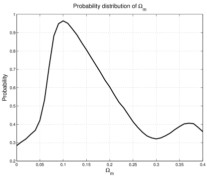
Figure 1: The marginalized likelihood distribution of $\Omega_{m0}$ for the spatially flat GCG model fitting result to SN Ia data.

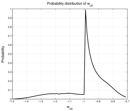
Figure 2: The marginalized likelihood distribution of $w_{c0}$ for the spatially flat GCG model fitting result to SN Ia data.

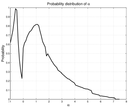
Figure 3: The marginalized likelihood distribution of $\alpha$ for the spatially flat GCG model fitting result to SN Ia data.

IV Age Fitting Results

Follow age , we define the look back time as

$$t_{L}(z)={1\over H_{0}}\int_{0}^{z}\frac{dx}{(1+x)E(x)}.$$ (21)

The current age of the Universe is $t_{0}=t_{L}(\infty)=14.4\pm 1.4$ Gyr age ; age1 . The age of an object $i$ at redshift $z$ is given by

$$t_{i}(z)={1\over H_{0}}\int_{z}^{z_{F}}\frac{dx}{(1+x)E(x)}=t_{L}(z_{F})-t_{L}(z),$$ (22)

where $z_{F}$ is the formation redshift when the object was born. From Eq. (22), we see that

$$t_{L}(z)=t_{L}(z_{F})-t_{i}(z)=t_{0}-t_{i}(z)-[t_{0}-t_{L}(z_{F})],$$

where the delay factor $df=t_{0}-t_{L}(z_{F})$ gives the information about the unknown formation redshift $z_{F}$. As in age , we also assume that the delay factor is the same for all the objects. The parameters in the GCG model are determined by minimizing

$$\tilde{\chi}^{2}=\left(\frac{t_{0}-t^{\rm obs}_{0}}{\sigma_{t}}\right)^{2}+\sum_{i}\frac{[t_{L}(z_{i})-t_{0}^{\rm obs}+t_{i}^{\rm obs}(z_{i})+df]^{2}}{\sigma^{2}_{t}+\sigma_{c}^{2}},$$ (23)

where $t_{0}^{\rm obs}=14.4$ Gyr, $\sigma_{t}=1.4$ Gyr and $\sigma_{c}=1$ Gyr age . The nuisance parameter $df$ is marginalized over by integrating the likelihood function $L=\exp(-\tilde{\chi}^{2}/2)$ over all possible values of $df$. Alternatively, we marginalize over $df$ by minimizing $\tilde{\chi}^{2}$ over $df$ which gives $df=-\sum_{i}^{n}[t_{L}(z_{i})-t^{\rm obs}_{0}+t^{\rm obs}_{i}(z_{i})]/n$. Because we already have four parameters: $\Omega_{m0}$, $\Omega_{k}$, $w_{c0}$ and $\alpha$ in the model, we use $H_{0}^{-1}=9.78h^{-1}$ Gyr with $h=0.72$ given by HST Key project hst . The observational data for the age of cluster sample is given in age . We reproduce the data in Table 2.

$z$	0.1	0.25	0.6	0.7	0.8	1.27
$t_{i}(z)$ (Gyr)	10.65	8.89	4.53	3.93	3.41	1.6
$t_{0}^{\rm obs}-t_{i}(z)$ (Gyr)	3.75	5.51	9.87	10.47	10.99	12.8

Table 2: The age data from Ref. age

For the spatially flat LCDM model, the best fit result is $\Omega_{m0}=0.20^{+0.08}_{-0.06}$ with $\chi^{2}=1.0$. Due to the sparse of the data, the result is not as good as that from SN Ia. For the spatially flat GCG model, the best fit results are: $\Omega_{m0}\sim 0$, $w_{c}\sim-1$ and $\alpha=6.53$. Again, the data does not favor GCG model over LCDM model.

V Conclusions

In this paper, we studied the GCG model which provides a phenomenological mechanism of unifying dark matter and dark energy. We explored a larger parameter space for the GCG model. Instead of studying the usual parameter range $0\leq\alpha\leq 1$, we extended the parameter space to be $\alpha>-1$ with some physical constraints on the parameters. We found that the parameters had bimodal distributions in general. The constraints from Type Ia SN data and the age data of clusters do not favor the GCG model over the simplest LCDM model from the standards of the Akaike information criterion and the Bayesian information criterion. Therefore, the current observations are consistent with both the GCG model and the LCDM model. Moreover, the flat model fits the observational data better. The only benefit of the GCG model is that it may provide a phenomenological mechanism of unifying dark matter and dark energy.

- (1) S. Perlmutter et al, Astrophy. J. 517 (1999) 565; P.M. Garnavich et al, Astrophys. J. 493 (1998) L53; A.G. Riess et al, Astron. J. 116 (1998) 1009.
- (2) D.N. Spergel et al, Astrophys. J. Suppl. 148 (2003) 175.
- (3) A.G. Riess, Astrophys. J. 607 (2004) 665.
- (4) C. Wetterich, Nucl. Phys. B 302 (1988) 668; B. Ratra and P. J. E. Peebles, Phys. Rev. D 37 (1988) 3406; Rev. Mod. Phys. 75 (2003) 559; R. R. Caldwell, R. Dave and P.J. Steinhardt, Phys. Rev. Lett. 80 (1998) 1582; I. Zlatev, L. Wang and P. J. Steinhardt, Phys. Rev. Lett. 82 (1999) 896.
- (5) C. Armendariz-Picon, T. Damour and V. Mukhanov, Phys. Lett. B 458 (1999) 209; C. Armendariz-Picon, V. Mukhanov and P.J. Steinhardt, Phys. Rev. Lett. 85 (2000) 4438; Phys. Rev. D 63 (2001) 103510.
- (6) A. Sen, JHEP 0204 (2002) 048; G.W. Gibbons, Phys. Lett. B 537 (2002) 1; T. Padmanabhan and T.R. Choudhury, Phys. Rev. D 66, 081301 (2002); J.S. Bagla, H.K. Jassal and T. Padmanabhan, ibid. 67, 063504 (2003); T. Padmanabhan and T.R. Choudhury, Mon. Not. Roy. Astron. Soc. 344, 823 (2003); P.S. Piao, R.G. Cai and Y.Z. Zhang, Phys. Rev. D 66 (2002) 121301.
- (7) A. Cohen, D. Kaplan and A. Nelson, Phys. Rev. Lett. 82 (1999) 4971; P. Hořava and D. Minic, Phys. Rev. Lett. 85 (2000) 1610; S. Thomas, Phys. Rev. Lett. 89 (2002) 081301; S.D.H. Hsu, Phys. Lett. B 594 (2004) 13; M. Li, hep-th/0403127; K. Ke and M. Li, hep-th/0407056; B. Wang, E. Abdalla and R.K. Su, hep-th/0404057; R.G. Cai, JCAP 0402 (2004) 007; Q-G. Huang and Y. Gong, JCAP 0408 (2004) 006; Y. Gong, Phys. Rev. D 70 (2004) 064029.
- (8) G.R. Dvali, G. Gabadadze and M. Porrati, Phys. Lett. B 485, 208 (2000); C. Deffayet, G.R. Dvali and G. Gabadadze, Phys. Rev. D 65, 044023 (2002); Z.H. Zhu, M. Fujimoto, Astrophys. J. 581, 1 (2002); 585, 52 (2003); 602, 12 (2004); Z.H. Zhu, M. Fujimoto and X.T. He, Astrophys. J. 603, 365 (2004); Z.H. Zhu and J.S. Alcaniz, astro-ph/0404201; B. Wang, Y. Gong and R.K. Su, hep-th/0408032; Y. Gong, X.M. Chen and C.K. Duan, Mod. Phys. Lett. A 19, 1933 (2004).
- (9) A. Kamenshchik, U. Moschella and V. Pasquier, Phys. Lett. B 511, 265 (2001).
- (10) M. Bento, O. Bertolami and A.A. Sen, Phys. Rev. D 66, 043507 (2002).
- (11) H.B. Sandvik, M. Tegmark, M. Zaldarriaga and I. Waga, Phys. Rev. D 69, 123524 (2004).
- (12) L.M.G. Beça, P.P. Avelino, J.P.M. de Carvalho and C.J.A.P. Martins, Phys. Rev. D 67, 101301 (2003).
- (13) J.C. Fabris, S.V.B. Gonsalves and P.E. de Souza, GRG 34, 53 (2002); N. Bilic, G.B. Tupper and R. Violler, Phys. Lett. B 535, 17 (2002); V. Gorini, A. Kamenshchik and U. Moschella, Phys. Rev. D 67, 063509 (2003); U. Alam, V. Sahni, T.D. Saini and A.A. Starobinsky, Mon. Not. Roy. Astron. Soc. 344, 1057 (2003); V. Gorini, A. Kamenshchik, U. Moschella and V. Pasquier, Phys. Rev. D 69, 123512 (2004); gr-qc/0403062.
- (14) T. Multamäki, M. Manera and E. Gaztañaga, Phys. Rev. D 69, 023004 (2004); O. Bertolami, A.A. Sen, S. Sen and P.T. Silva, astro-ph/0402387; J.G. Hao and X.Z. Li, astro-ph/0404154; S. Nesseris and L. Perivolaropoulos, Phys. Rev. D 70, 043531 (2004); S.K. Srivastava, astro-ph/0407048; P.P. Avelino et al., astro-ph/0208528; D. Carturan and F. Finelli, Phys. Rev. D 68, 103501 (2003); A.K.D. Evans, I.K. Wehus, Ø. Grøn and Ø. Elgarøy, astro-ph/0406407; L.P. Chimento, Phys. Rev. D 69, 123517 (2004); Z.H. Zhu, Astron. & Astrophys. 423, 421 (2004).
- (15) Y. Gong and C.K. Duan, Class. Quantum Grav. 21, 3655 (2004); Mon. Not. Roy. Astron. Soc. 352, 847 (2004); T. Barreiro and A.A. Sen, astro-ph/0408185.
- (16) M.C. Bento, O. Bertolami and A.A. Sen, Phys. Lett. B 575, 172 (2003).
- (17) T. Chiba and T. Nakamura, Prog. Theor. Phys. 100, 1077 (1998).
- (18) V. Sahni, T.D. Saini, A.A. Starobinsky and U. Alam, JETP Lett. 77, 202 (2003).
- (19) H. Akaike, IEEE Trans. Auto. Control, 19, 716 (1974); G. Schwarz, Annals of Statistics, 5, 461 (1978); P.S. Corasaniti et al., astro-ph/0406608.
- (20) C.L. Bennett, Astrophys. J. Supp. 148, 1 (2003).
- (21) S. Capozziello, V.F. Cardone, M. Funaro and S. Andreon, astro-ph/0410268.
- (22) R. Rebolo et al., astro-ph/0402466.
- (23) W.L. Freedman et al., Astrophys. J., 553, 47 (2001).