Standard model atmospheres for A-type stars and non-LTE effects

Abstract

The current status of NLTE model atmosphere calculations of A type stars is reviewed. During the last decade the research has concentrated on solving the restricted NLTE line formation problem for trace elements assuming LTE model atmospheres. There is a general lack of calculated NLTE line blanketed model atmospheres for A type stars, despite the availability of powerful methods and computer codes that are able to solve this task. Some directions for future model atmosphere research are suggested.

1 Introduction

Compared to the atmospheres of hotter O and B stars that have stellar winds and to atmospheres of cooler F and G stars that have convective atmospheres, the atmospheres of A-type stars are relatively quiet, which enables the presence of various interesting phenomena. This calmness of atmospheres leads to the development of a number of different chemical peculiarities and magnetic field structures on long time scales.

There exists a widely used grid of line blanketed LTE model atmospheres (Kurucz [1993], Castelli & Kurucz [2003]), which is also extensively used for A stars. Besides this grid, several attempts to remove the inconsistent assumption of LTE have been performed. The very first NLTE calculation of a cool B star, which can be somehow understood as a first step toward A star modelling, was performed by Auer & Mihalas ([1970]). The domain of A star temperatures was first reached by Kudritzki ([1973]) and Frandsen ([1974]). A grid of NLTE model atmospheres of stars with $10000\,{\mathrm{K}}\leq\mbox{$T_{\mathrm{eff}}$}\leq 15000\,{\mathrm{K}}$ (thus also including a part of the A star domain) was calculated by Borsenberger & Gros ([1978]). A great stride was made by Hubený ([1980], [1981]), who studied in detail the effect of the L$\alpha$ line on the NLTE model atmospheres of A stars and applied his code to star Vega. A detailed analysis of the physics which is contained in releasing the assumption of LTE was presented by Hubený ([1986]). First NLTE line blanketed model atmospheres of A stars were calculated using a method of superlevels and superlines by Hubeny & Lanz ([1993]). Unfortunately, although there was great progress in calculating NLTE model atmospheres for hot stars and for white dwarfs, calculations of NLTE model atmospheres of A stars are very rare. The only attempt of a NLTE model atmosphere of an A-type star was the model calculated by Hauschildt et al. ([1999]) for parameters corresponding to Vega. The authors announced a grid of NLTE models to be published, but till now nothing appeared.

The inherent reason which stands tacitly behind the lack of calculated NLTE A star model atmospheres is in the different scaling properties of the atmospheres of this stellar type. The atmosphere of A stars have very extended line formation regions meaning that different lines form at very different depths (cf. Fig. 1 in Lanz & Hubeny, [1993]). Therefore they are very difficult to describe by a simple standard depth discretization as compared to O stars and white dwarfs, and hence a much more elaborate depth scale has to be used. Our own experience shows that there are severe convergence problems caused by improper depth scaling and only a tremendous number of depth points helped.

2 Basic equations for NLTE model atmospheres

A solution of a model atmosphere problem means taking the basic input values of stellar luminosity $L$, stellar radius $R$, and stellar mass $M$ (or, equivalently for the usual plane-parallel case effective temperature $T_{\mathrm{eff}}$ and gravitational acceleration at the stellar surface $g$), adding physical laws that are important in the stellar atmosphere (a principal ingredient), and calculating the space distribution of various physical quantities (temperature $T(\vec{r})$, electron density $n_{e}(\vec{r})$, population numbers $n_{i}(\vec{r})$, density $\rho(\vec{r})$, velocity field $\vec{v}(\vec{r})$, etc.). This procedure is often being performed in substeps. The first step is the determination of $T$, $n_{e}$, $\rho$, and $n_{i}$ for the most important opacity sources. The second (optional) step is the determination of $n_{i}$ for the minor abundant species, often referred to as trace elements. The final step in this process is the calculation of the theoretical emergent radiation which may be then compared to the observed one.

A standard model atmosphere here is a static one-dimensional (plane-parallel or spherically symmetric) atmosphere in hydrostatic, radiative, and statistical equilibrium. To calculate such a model atmosphere we need to solve the radiative transfer equation (to determine the radiation field $I$), the hydrostatic equilibrium equation (to determine $\rho$), the energy equilibrium equation (to determine $T$), and the statistical equilibrium equations (to determine $n_{i}$).

2.1 Radiative transfer equation

The radiative transfer equation is the principal equation for model atmosphere calculations. Regardless of the geometrical approximation which is adopted, the basic solution of the radiative transfer equation is performed along a ray, which reads

$${\mathrm{d}I_{\nu}(r)\over\mathrm{d}s}=-\chi_{\nu}(r)I_{\nu}(r)+\eta_{\nu}(r).$$ (1)

Usually the simplest possibility, i.e. the plane-parallel atmosphere, is being used for the modelling of stellar atmospheres, basically due to its relative simplicity.

2.1.1 Formal solution

By formal solution of Equation (1) we mean the solution for a given opacity and emissivity. Such a solution may be performed using either differential or integral methods. The latter are especially useful for the multidimensional case. The inconsistency of the formal solution is that opacity $\chi_{\nu}$ and emissivity $\eta_{\nu}$ are not given, but in the process of solving the model atmosphere problem they depend on temperature, density, and radiation field, which are to be determined when solving the radiative transfer equation. However, the formal solution remains at the heart of each model atmosphere code (see Auer [2003]).

2.1.2 Approximate solution using ALO

The process of the formal solution may be expressed using the $\Lambda$-operator

$$J_{\nu}=\Lambda_{\nu}S_{\nu}.$$ (2)

This expression may be used in an iterative process, where the source function $S_{\nu}$ is determined by solving the other constraint equations of hydrostatic, energy, and statistical equilibria. As has been shown, such a process, however effective for the optically thin cases of molecular clouds (cf. Dickel & Auer [1994]), fails to produce a convergent solution for the optically thick cases of stellar atmospheres (see Auer [1984]). This problem has been overcome using the Newton Raphson method for model stellar atmospheres by Auer & Mihalas ([1969]). As an efficient alternative, an approximate $\Lambda$-operator $\Lambda^{\ast}_{\nu}$ may be used,

$$J_{\nu}=\mbox{$\Lambda^{\ast}_{\nu}$}S_{\nu}+\left(\Lambda_{\nu}-\mbox{$\Lambda^{\ast}_{\nu}$}\right)S_{\nu}$$ (3)

The operator $\Lambda^{\ast}_{\nu}$ is constructed in such a way that it contains the basic physics of the problem and is simply calculable. The most efficient method is to calculate this operator consistently with the numerical method used for the formal solution, like it has been described by Rybicki & Hummer ([1991]) or Puls ([1991]). Then the radiation field is determined by an iterative process,

$$J_{\nu}^{(n)}=\mbox{$\Lambda^{\ast}_{\nu}$}\left[S_{\nu}\left(J_{\nu}^{(n)}\right)\right]+\left(\Lambda_{\nu}-\mbox{$\Lambda^{\ast}_{\nu}$}\right)\left[S_{\nu}\left(J_{\nu}^{(n-1)}\right)\right]$$ (4)

where $(n)$ means the current iteration step and $(n-1)$ the previous one.

2.2 Energy equilibrium

The energy equilibrium equations determine the temperature structure. They describe the basic energy balance in the atmosphere. For the case of static atmospheres, the equation of radiative equilibrium,

$$\int_{0}^{\infty}\left(\kappa_{\nu}J_{\nu}-\eta_{\nu}\right)d\nu=\int_{0}^{\infty}\kappa_{\nu}\left(J_{\nu}-S_{\nu}\right)d\nu=0,$$ (5)

which simply describes the radiative energy balance, is usually being used. However, this equation does not guarantee the radiative flux conservation, which results in an incorrect temperature structure at large optical depths. Therefore, another form, which comes from $\nabla\cdot\vec{\cal{F}}=0$, is to be used at large optical depths. Better numerical properties of the scheme may be achieved if a linear combination of these equations is considered, as was first done by Hubeny & Lanz ([1995]). Another improvement of convergence properties, especially useful at low continuum optical depths where strong lines are still present, was introduced by Kubát et al. ([1999]) where a thermal balance of electrons instead of the radiative equilibrium equation is used.

Then three different equations may be used in the stellar atmosphere to take into account energy equilibrium. In the deepest layers, the differential form of radiative equilibrium is used. In the middle parts, where continuum radiation is formed, the integral form of radiative equilibrium works well. In the outer parts where optically thick lines coexist with an optically thin continuum (which is the case of A star atmospheres), the thermal balance of electrons works best. A more detailed discussion with the numerical properties of these methods may be found in Kubát ([2003a, 2003b]).

2.3 Equations of statistical equilibrium

The equations of statistical equilibrium are the key equations both for the NLTE model atmosphere and line formation problems. The set of equations for statistical equilibrium for the static case may be written as

$$n_{i}\sum_{l}(R_{il}+C_{il})-\sum_{l}n_{l}(R_{li}+C_{li})=0$$ (6)

Radiative rates $R_{il}$ are those responsible for the NLTE effects, since they introduce nonlocal interaction and they alter the level population irrespective of local equilibrium conditions. They move the gas outside thermodynamic equilibrium. On the other hand, for an equilibrium (Maxwellian) electron velocity distribution (which is the common case), collisional rates reintroduce thermodynamic equilibrium. The balance between collisional and radiative rates determines the applicability of the LTE approximation. If collisions dominate, then the LTE approximation is feasible. If radiative transitions dominate, which is the case in A star atmospheres, then equations of statistical equilibrium need to be solved if we want to obtain the correct population numbers.

Since the system of rate equations is linearly dependent, we have to close it with some other condition. For a reference (usually, but not necessarily hydrogen) atom either particle conservation equation $\sum_{k}N_{k}=N-n_{e}$ or charge conservation equation $\sum_{k}\sum_{j}q_{j}N_{jk}=n_{e}$ are used. For other atoms, the abundance equation $N_{k}=Y_{k}N_{r}$ is usually used. Detailed forms of the equations may be found, e.g., in Kubát ([1997]).

2.4 Solution of the system of equations

The whole system of equations is usually solved using a Newton-Raphson iteration scheme, which in modeling stellar atmospheres used to be referred to as linearization (Auer & Mihalas [1969]). The radiation field is linearized as well, or it can be included using approximate lambda operators (see Eq. 4), as has been first done by Werner ([1986]). Excellent reviews of ALI methods of model atmosphere solutions are provided by Hubeny ([2003]) and Werner et al. ([2003]). In addition, an implicit linearization of $b$-factors saves additional computer time and memory (Anderson [1987]). The whole process may be accelerated using either Kantorovich (see Hubeny & Lanz [1992]) or Ng acceleration (see Auer [1991]).

2.5 Line blanketing

Line blanketing is caused by enormous amounts of spectral lines in the UV region ($\sim 10^{7}$), mostly of iron and nickel. This enormous amount of lines causes radiation to be absorbed in the UV and reemitted in the visible region, thus changing the emergent flux and atmospheric structure significantly.

There are two main approaches to line blanketing under the simplifying assumption of LTE, the ODF (Opacity Distribution Function) and OS (Opacity Sampling).

If we do not use the assumption of LTE, we have to solve the equations of statistical equilibrium to obtain the correct population numbers for all levels. This task is relatively simple for simple atoms (like He), but becomes difficult for atoms with a complicated level structure, like iron. In order to cope with the complexity of these atoms, Anderson ([1989]) introduced the concept of superlevels and superlines. A superlevel is a level which is created by grouping several individual levels. In order to achieve a real simplification, it is useful to group the levels in such a manner that the relative population distribution inside the superlevel obeys the LTE distribution. Thus, this grouping is done according to the energy, $E_{i}$, of individual levels (Anderson [1989], Dreizler & Werner [1993]). A more sophisticated grouping according to $E_{i}$ and parity was done by Hubeny & Lanz ([1995]). Dreizler & Werner ([1993]) used opacity sampling in their calculations, whereas Hubeny & Lanz ([1995]) used the NLTE opacity distribution function.

2.6 LTE versus NLTE

Since the beginning of the NLTE calculations there is a battle between ’LTE people’ and ’NLTE people’, which of the approaches is better. If NLTE model atmosphere is calculated as easily as the LTE one, there would be no discussion and everybody would use the NLTE one. However, this is not the case and it is much more difficult to calculate a NLTE model than the LTE model. Two conflicting aims enter the scene. The first one is to analyse as many stars as possible, which can be hardly done using NLTE models. The second one is to study stars as accurately as possible, which can be hardly done using LTE models.

For the case of LTE it is relatively easy to handle line blanketing, since one neglects the effect of radiation on atomic population numbers, which saves computing time enormously. On the other hand for a more general case of NLTE, including line blanketing is computationally expensive, albeit nowadays it is possible to handle NLTE calculations using sophisticated numerical methods and contemporary computers. However, for extended atmospheres the reliability of LTE decreases and one is forced to use NLTE.

To avoid repeated calculations of complicated model atmospheres one may take the advantage of precomputed grids. However, one has to keep in mind that using such grids, which were calculated under certain physical assumptions, always limits the results by these assumptions.

3 NLTE line formation calculations

Table 1: List of NLTE calculations for a given LTE model atmosphere for A stars

Ion	reference	code	comment on included levels and transitions
He i	Takeda ([1994])	3	calculations for Deneb; 88 levels
Li i	Mashonkina et al. ([2002])	4
Li i/ii	Shavrina et al. ([2001])		20 levels
C i	Takeda ([1992b])	3	129 levels, 2351 radiative transitions
	Venn ([1995])	2	83 levels
	Rentzsch-Holm ([1996b])	2	83 levels, 63 transitions
	Paunzen et al. ([1999])	2	83 levels, 63 transitions
C i/ii	Przybilla et al. ([2001b])	1	C i levels with $n\leq 9$, C ii levels with $n\leq 4$
N i	Takeda ([1992b])	3	119 levels, 2119 radiative transitions
	Sadakane et al. ([1993])	3	used model atom of Takeda ([1992b])
	Takeda & Takada-Hidai ([1995])	3	used model atom of Takeda ([1992b])
	Takada-Hidai & Takeda ([1996])	3	used model atom of Takeda ([1992b])
	Venn ([1995])	2	93 levels, 189 transitions
	Lemke & Venn ([1996])	2	93 levels, 189 radiative transitions
	Rentzsch-Holm ([1996a])	2	96 levels, 82 transitions
N i/ii	Przybilla & Butler ([2001])	1	N i levels with $n\leq 7$, N ii levels with $n\leq 6$
O i	Takeda ([1992a, 1997])	3	86 levels, 294 radiative transitions
	Takeda & Takada-Hidai ([1998])	3	86 levels, 294 radiative transitions
	Takeda et al. ([1999])	3	calculations from Takeda ([1997]) for CP stars
	Paunzen et al. ([1999])	2	15 levels
	Przybilla et al. ([2000])	1	all levels below excitation energy
Na i	Takeda & Takada-Hidai ([1994])	3	calculations for A supergiants, 92 levels, 178 radiative transitions
	Mashonkina et al. ([2000])	4	solution for $\mbox{$T_{\mathrm{eff}}$}=4000-12\,000\,{\mathrm{K}}$, 21 levels
Mg i	Shimanskaya et al. ([2000])	4	solution for $\mbox{$T_{\mathrm{eff}}$}=4500-12000\,{\mathrm{K}}$, 50 levels
	Idiart & Thévenin ([2000])	5	104 levels, 980 radiative transitions
Mg i/ii	Przybilla et al. ([2001a])	1	all levels with $n\leq 10$
S i	Takeda & Takada-Hidai ([1995])	3	56 levels, 173 radiative transitions
	Takada-Hidai & Takeda ([1996])	3	56 levels, 173 radiative transitions
K i	Ivanova & Shimanskii ([2000])	4	solution for $\mbox{$T_{\mathrm{eff}}$}=4000-10\,000\,{\mathrm{K}}$, 36 levels
Ca i	Idiart & Thévenin ([2000])	5	84 levels, 483 transitions
Ti ii	Becker ([1998])	1	complete model atom, using superlevels
Fe ii	Becker ([1998])	1	complete model atom, using superlevels
Fe i/ii	Rentzsch-Holm ([1996b])	2	79+20 levels, 52+23 lines
	Thévenin & Idiart ([1999])	5	256+190 levels, 2117+3443 lines
Sr ii	Belyakova et al. ([1999])	4	solution for $\mbox{$T_{\mathrm{eff}}$}=4000-12\,000\,{\mathrm{K}}$, 41 levels
Nd ii/iii	Mashonkina et al. ([2004])	1	247+69 levels

Computer codes used for calculations: 1 – DETAIL (Giddings [1981]); 2 – Kiel (Steenbock & Holweger [1984]); 3 – Takeda ([1991]); 4 – NONLTE3 (Sakhibullin [1983]); 5 – MULTI (Carlsson [1986]);

Calculations of full NLTE model atmospheres of A type stars is a difficult task. Due to a large span of line formation regions down to optical depths in the continuum of about $10^{-9}$, the numerical procedure becomes extremely unstable and calculations need special care. That is why people started to solve easier task of NLTE line formation for a given model atmosphere. A necessary condition for such calculation to be reasonable, is negligible influence of the ion on the ionization balance and, consequently, on the global structure of the atmosphere. Such elements are being referred to as trace elements.

Contemporary NLTE analysis of A stars are mainly concerned with solving the statistical equilibrium equations for trace elements for a given (mostly LTE) model atmosphere. These kind of calculations have already been reviewed by Hubený ([1986]) and Hubeny & Lanz ([1993]), so only new calculations that appeared after the last review are listed in Table 1. We did our best to mention all calculations. In the case we unintentionally omitted some, we apologize for it.

There are several codes available for this purpose. They use slightly different numerical techniques, basic differences are in the treatment of the radiation field. Both the accelerated lambda iteration and complete linearization methods are used. A comparison of results from different codes for Vega (and Sun) was presented by Kamp et al. ([2003]), who found large differences in the results different codes. Therefore we added to Table 1 an indication which code was used.

4 Beyond standard model atmospheres

4.1 Nonthermal collisional rates

In standard NLTE calculations only the radiation field and level populations are allowed to deviate from their equilibrium values. The velocity distribution of individual species is still assumed to be in equilibrium. Collisional rates are then calculated as an average over the Maxwellian electron velocity distribution,

$$C_{ij}=n_{e}\int_{v_{0}}^{\infty}\sigma_{ij}(v)f(v)v\mathrm{d}v.$$ (7)

Thus in equilibrium there holds a relation between collisional rates up and down (excitation/deexcitation or ionization/recombination),

$$n_{i}^{\ast}C_{ij}=n_{j}^{\ast}C_{ji}.$$ (8)

If the velocity distribution is not Maxwellian (e.g. in electron beams formed in the Sun during flares – cf. Kašparová & Heinzel [2002]), then the equation (8), which expresses the equilibrium condition, is not valid. In such a case the collisions may cause level population numbers to differ from the LTE values, which has an observable effect on the line profiles. The nonthermal collisional term may be considered as another source of NLTE effects. Such effects are present in the Sun, where the electron beams are formed after magnetic reconnection. There is also a possibility that they may be present in magnetic A stars, where releasing magnetic energy in eruptive events like flares may be expected as well.

4.2 Magnetic fields

Inclusion of magnetic fields into model atmosphere calculations have been done only occasionally. An important attempt in calculating a model atmosphere with a magnetic field was done by Carpenter ([1985]), who found changes in the net gravity and pressure distribution due to the magnetic field. The most consistent model so far was recently developed by Valyavin et al. ([2004]), who assumed LTE and included the Lorentz force into the equation of hydrostatic equilibrium. A historical overview of magnetic model atmosphere calculations is also presented there.

4.3 Diffusion

An important aspect of A star atmospheres is the fact that atmospheres of a good fraction of stars of this stellar spectral type are extremely quiet. Such quiet atmospheres without significant global motions like global convection and stellar winds enable long time scale processes of diffusion and gravitational settling to take place. Diffusion occurs not only in the presence of magnetic field (note the effect of enhancing radiative acceleration in polarized radiation field and the effect of ambipolar diffusion, Babel & Michaud [1991a, 1991b]), but also due to different sensitivities of various atoms and ions to incoming radiation. Radiative diffusion is able to explain various chemical peculiarities in CP stars and is also responsible for the isotopic shift effect (Aret & Sapar [2002]). However, consistent NLTE model atmospheres that take into account radiative diffusion processes are still missing for A type stars. NLTE model atmospheres with diffusion were calculated by Dreizler & Shuh ([2003]) for white dwarfs, where diffusion processes are also important. The physical process of diffusion is reviewed in detail elsewhere in these proceedings (Michaud).

4.4 Extended atmospheres

Plane-parallel model atmospheres are also being used for NLTE modeling of atmospheres of A-type supergiants (e.g., Kudritzki [1973]). However, they do not describe the limb darkening correctly. A-type supergiants have also stellar winds and show P Cyg line profiles, therefore it is impossible to describe them using plane parallel atmospheres. Also, wind models of A stars are not calculated too often. Multicomponent hydrodynamic radiatively driven wind models for A stars were calculated by Babel ([1995]). Another radiation driven wind model was calculated by Achmad et al. ([1997]), but they did not take into account non-LTE effects. Generally, for extended atmospheres the NLTE effects are stronger. An attempt to calculate spherically symmetric NLTE model atmospheres with a stellar wind of Deneb was done by Aufdenberg et al. ([2002]). However, as the authors note, they were not able to fit the observed H$\alpha$ line profile. Work on developing consistent NLTE wind models of A supergiants is currently in progress (Krtička & Kubát, these proceedings).

4.5 Limb darkening

An important property of emergent radiation from stellar atmospheres is the angle dependence of the specific intensity $I(\theta)$, usually called limb darkening. Approximate limb darkening laws are often used (see, e.g., Allen, [1963] or Gray, [1976]). These approximate laws don’t describe the angular dependence of the specific intensity very well even in the case of thin stellar atmospheres. In addition, limb darkening is strongly frequency dependent (Hadrava & Kubát [2003]), and in the center of a line, even limb brightening instead of darkening may appear, as can be seen in Figure 1.

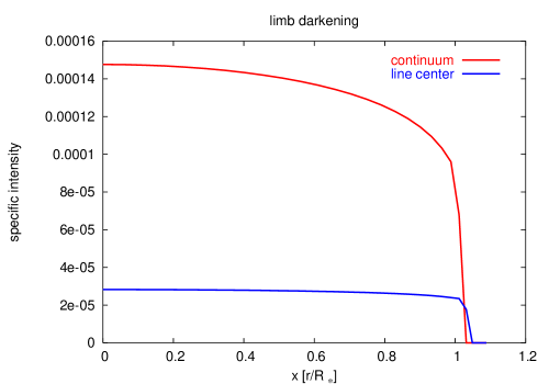
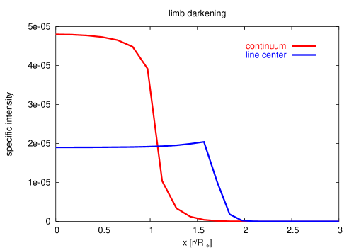
Figure 1: The comparison of limb darkening for the thin atmosphere (left panel) and the extended atmosphere (right panel). These results were obtained from the Korčáková & Kubát code ([2003]).

This effect becomes very strong especially for extended stellar atmospheres.

For a correct description of limb darkening it is necessary to use model atmospheres with a better geometry than plane-parallel. This has been done by Claret & Hauschildt ([2003]), who, using a spherically symmetric code, calculated limb darkening for a grid of model atmospheres from A to G spectral types.

Knowledge of an accurate limb darkening law is necessary for detecting stellar spots (see Kjurkchieva, [1989]). It is also very important for the analysis of interferometric measurements, as well as for the correct treatment of stellar rotation. Luckily, eclipses from binaries (e.g., Twigg [1979]), and the gravitational microlensing effect (Heyrovský [2003]) measurements of limb darkening are possible for at least some of the distant stars.

4.6 Rotation

Stellar rotation is usually being accounted by convolving the rotation profile with the static line profile (see Gray [1976]). This technique is inaccurate not only due to using only approximate limb darkening laws, but also because the dependence of limb darkening on frequency as well as gravity darkening are neglected. A more accurate method is to integrate the static intensity over the rotating disc of the star, where gravity darkening can also be included. A “simple” way of including gravity darkening in this integration is described by Collins ([1963]). This method was used by Gulliver et al. ([1994]) to determine the rotation of Vega.

Stellar rotation is not like a rigid body rotation, as it is usually assumed, but it is probably differential. Until now, there are only few measurements of differential rotation. Unfortunately, in many works, the authors use the simplest form of the limb darkening law and the obtained results can be used only with reservations.

For an exact description of stellar rotation the plane-parallel model atmosphere is insufficient. It is necessary to use a hydrodynamic multidimensional model atmosphere, at least an axially symmetric one together with the correct description of the radiation field. Recently, we started to work on such a model (Korčáková et al., these proceedings).

5 Conclusions

Full NLTE model atmospheres of A stars are difficult to calculate, since the lines of different ions form at very different depths, and therefore there is a need for a huge amount of depth points to resolve all line formation regions sufficiently. Only LTE model atmospheres together with NLTE calculations for individual ions have been calculated in significant amounts. This underlines the need for more intensive calculations of NLTE model atmospheres of A stars. Adding consistently new different physical processes to NLTE model atmospheres calculations, such as diffusion (see Michaud, these proceedings), magnetic fields (see Moss, these proceedings), and more accurate treatment of convection zones (see Kupka, these proceedings), is necessary. This is the real challenging task the near future.