Limits on the Transverse Velocity of the Lensing Galaxy in Q2237$+$0305 from the Lack of Strong Microlensing Variability

We present a method for the determination of upper limits on the transverse velocity of the lensing galaxy in the quadruple quasar system Q2237$+$0305, based on the lack of strong microlensing signatures in the quasar lightcurves. The limits we derive here are based on four months of high quality monitoring data, by comparing the low amplitudes of the lightcurves of the four components with extensive numerical simulations. We make use of the absence of strong variability of the components (especially components B and D) to infer that a “flat” time interval of such a length is only compatible with an effective transverse velocity of the lensing galaxy of ${v_{\rm bulk}}\leavevmode\nobreak\ \leq\leavevmode\nobreak\ 630$ km/s for typical microlenses masses of $M_{\rm\mu lens}=0.1M_{\odot}$ (or ${v_{\rm bulk}}\leavevmode\nobreak\ \leq\leavevmode\nobreak\ 2160$ km/s for $M_{\rm\mu lens}=1.0M_{\odot}$) at the 90% confidence level. This method may be applicable in the future to other systems.

1 Introduction

Measurements of the peculiar motions of galaxies can provide strong constraints on the nature of dark matter and the formation and evolution of structure in the Universe. Determining such ‘departures from the Hubble flow’, utilizing standard distance indicators as the Tully-Fisher relation for spirals and the $D_{n}-\sigma$ method for ellipticals (e.g., Peebles 1993), have proved to be quite difficult. While these measures provide radial peculiar motions, transverse peculiar motions are also required to fully constrain cosmological models. However, the determination of transverse velocities is an extremely difficult task, generally beyond the reach of current technology. Recently, Peebles et al. (2001) suggested the use of the space missions SIM and GAIA to estimate the transverse displacements of nearby galaxies. Roukema and Bajtlik (1999) claimed that transverse galaxy velocities could be inferred from multiple topological images, under the hypothesis that the ‘size’ of the Universe is smaller than the apparently ‘observable sphere’. In spite of these efforts, our knowledge of transverse motions of galaxies is currently very limited.

Dekel et al. (1990) showed that the local galaxy velocity field can be reconstructed assuming that this field is irrotational, and thus, the measurement of the transverse velocities could be used to test this assumption. In fact, the determination of transverse motions would be very useful to discuss the quality of the whole reconstruction. From another point of view, the reconstruction methods are powerful tools to estimate galactic transverse motions.

Grieger, Kayser and Refsdal (1986) had suggested using gravitational microlensing of distant quasars to determine the transverse velocity of the lensing galaxy via the detection of a ‘microlens parallax’ as the quasar is magnified during a caustic crossing (see also Gould 1995). For the determination of this parallax, however, ground-based monitoring is not sufficient, it requires parallel measurements from a satellite located at several AU in addition.

The gravitational lens Q2237$+$0305 consists of four images of a quasar at a redshift of $z_{q}=1.695$, lensed by a low redshift ($z_{g}=0.039$) spiral galaxy (Huchra et a. 1985). Photometric monitoring revealed uncorrelated variability between the various images, interpreted as being due to gravitational microlensing (Irwin et al. 1989). This interpretation was confirmed with dedicated monitoring programs (e.g., Østensen et al. 1996; Woźniak et al. 2000a,b; Alcalde et al. 2002). Q2237$+$0305 is the best studied quasar microlensing system. With ten years of monitoring data, Wyithe et al. (1999) used the derivatives of the observed microlensing lightcurves to put limits on the lens galaxy tranverse velocity of Q2237+0305. Very recently, Kochanek (2004) developed a method for analysing microlensing lightcurves based on a $\chi^{2}$ statistics which includes the transverse velocity of the source as an output parameter.

Here we present another method to determine upper limits on the transverse velocity of a lensing galaxy in a multiple quasar system. We apply it to Q2237$+$0305, based on a comparison between four months of high quality photometric monitoring of the four quasar images and intense numerical simulations. The details of the microlensing model and simulations are discussed in Section 2. In Section 3 we briefly present and review the lens monitoring results and outline our method to obtain limits on the transverse velocity. The results of this approach  – the constraints on the transverse velocity of the lensing galaxy –  are presented in Section 4 and discussed in Section 5. We include our conclusions in Section 6.

2 Microlensing background

2.1 Lens models of Q2237+0305

Several approaches have been employed in modeling the observed image configuration in Q2237+0305 (Schneider et al. 1988, Wambsganss and Paczyński 1994, Chae et al. 1998, Schmidt et al. 1998). These models provide the parameters relevant to microlensing studies: the surface mass density, $\Sigma$, and the shear, $\gamma$, at the positions of the different images. The former represents the mass distribution along the light paths projected into the lens plane, while the latter represents the anisotropic contribution of the matter outside the beams. We can normalize the surface mass density with the critical surface mass density (see Schneider et al. 1992 for more details),

$$\Sigma_{crit}=\frac{c^{2}}{4\pi G}\frac{D_{s}}{D_{d}D_{ds}}$$ (1)

where $D_{s}$, $D_{d}$ and $D_{ds}$ are the angular diameter distances between observer and source, observer and deflector and between deflector and source, respectively, $c$ is the velocity of light and $G$ is the gravitational constant. The resulting normalized surface mass density (also called convergence or optical depth) is expressed as $\kappa=\Sigma/\Sigma_{crit}$.

We use here two different sets of values for $\kappa$ and $\gamma$ for the four components (Tab. 1), corresponding to the Schneider et al. (1988) and the Schmidt et al. (1998) lens models, respectively. We will demonstrate using these two sets that slightly different values for the two local lensing parameters do not change the results, and hence that some scatter in $\kappa$ and $\gamma$ of the images does not affect the conclusions.

	Schneider et al. (1988)			Schmidt et al. (1998)
Image	$\kappa$	$\gamma$		$\kappa$	$\gamma$
A	0.36	0.44		0.36	0.40
B	0.45	0.28		0.36	0.42
C	0.88	0.55		0.69	0.71
D	0.61	0.66		0.59	0.61

Table 1: Two different sets of values for the surface mass density, $\kappa$, and the shear, $\gamma$, of the four images are used, in order to study the dependence of the result on the lens model (see References for details).

2.2 Simulations

We use the ray shooting technique (see Wambsganss 1990, 1999) to produce the 2-dimensional magnification maps for each of the gravitationally lensed images. All the mass is assumed to be in compact objects, with no smoothly distributed matter. This should be a good approximation for an old stellar population in the central part of the lens galaxy and a small amount of smooth matter would not introduce a significant difference in our results. All of the microlensing objects are assumed to have a mass of $M_{\rm\mu lens}$ and are distributed randomly over the lens plane. Taking into account the effect of the shear and the combined deflection of all microlenses, light rays are traced backwards from the observer to the source. This results in a non-uniform density of rays distributed over the source plane. The density of rays at a point is proportional to the microlensing magnification of a source at that position; hence the result of the rayshooting technique is a map of the microlensing magnification as a function of position in the source plane. The relevant scale factor, the Einstein radius in the source plane, is defined as

$$r_{E}=\left(\frac{4GM_{\rm\mu lens}}{c^{2}}\frac{D_{s}D_{ds}}{D_{d}}\right)^{1/2}.$$ (2)

Finally, the magnification pattern is convolved with a particular source profile for the quasar. Linear trajectories across this convolved map, therefore, result in microlensing light curves (see also Schmidt & Wambsganss 1998).

In general, the details of a quasar microlensing light curve depend on several unknown parameters: the masses and positions of the microlenses and the size, profile and effective transverse velocity of the source. For this reason, the comparison of the simulated microlensing lightcurves to the observed ones must be done in a statistical sense.

3 The Method

3.1 The idea in a nutshell

Before going into details of the method we use, we present a very simple hypothetical scenario to better illustrate the procedure. Generally, microlensing magnification maps possess significant structure, in particular they consist of an intricate web of very high magnification regions, the caustics. The density and the length of the caustics vary with the values of surface mass density $\kappa$ and shear $\gamma$. However, for a given pair of parameters $\kappa$ and $\gamma$, there is something like a typical distance between adjacent caustics (Witt et al. 1993), though with quite a large dispersion. For illustration purposes, we assume now that we have a magnification pattern with caustics that are equally spaced horizontal and vertical lines (see Fig. 1). Though this is far from being a realistic magnification pattern, its simplicity allows us to explain the relation between fluctuations in the microlensing lightcurves and the velocity of the source in simple terms. The pattern shows schematically the typical low (dark) and high (white) magnification areas, respectively. The length and width of the low magnification areas is exactly one unit length, $l_{\rm unit}$. If we compute the magnification along a linear track inside one of these regions, the resultant lightcurve will be flat. However, there is a maximum length for such flat lightcurves: there cannot be any flat lightcurves with lengths larger than $l_{\rm max}=\sqrt{2}\leavevmode\nobreak\ l_{\rm unit}$. Now suppose that this magnification map corresponds to a certain hypothetical gravitationally lensed system and we have a flat observed microlensing lightcurve corresponding to an observing period of $t_{\rm obs}$. Then we can calculate an upper limit for the velocity of the source: $V_{\rm max}=\sqrt{2}l_{\rm unit}/t_{\rm obs}$. Of course, the actual velocity could be (much) smaller than that; if only “flat” microlensing lightcurves existed, it could be as small as zero (measured caustic crossings will provide lower limits on the velocity).

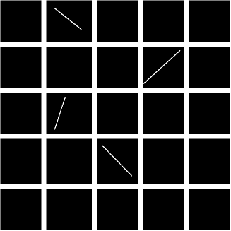
Figure 1: Idealized magnification pattern to illustrate the idea of the method: Black areas are low magnification zones, the regular grid of thick white lines represents the caustics (high magnification areas) and the thin white lines are example tracks due to the relative motion between source, lens and observer, which all would result in flat lightcurves.

As stated above, true microlensing magnification maps are much more complex than the idealized case presented in Figure 1. Nevertheless, we can determine an upper limit on the track lengths for a realistic magnification pattern in a statistical sense, by just replacing the fixed distance between the idealised caustics by the real distribution of caustic distances, and the perfectly flat parts for the regions between the caustics by the relatively flat real lightcurves. This way we can get an upper limit $l_{\rm upper}$ on the track lengths (in $r_{E}$) that is consistent with the observed variability. Since we know the duration of the observing period $t_{\rm obs}$ from the actual monitoring campaign, it is straightforward to obtain the upper limit on the transverse velocity for assumed values of the lens mass $M_{\rm\mu lens}$ and the source size/profile: $V_{\rm upper}=l_{\rm upper}/t_{\rm obs}$.

Although the effective transverse velocity has contributions from all three components source, lens, and observer as shown below, for the system Q2237+0305, the effective transverse velocity is dominated by the effective transverse velocity of the lensing galaxy (Kayser et al. 1986).

3.2 Monitoring Observations of Q2237+0305 to be compared with

This study employs the results of the GLITP (Gravitational Lenses International Time Project) collaboration which monitored Q2237+0305 from October 1st, 1999 to February 3rd, 2000, using the 2.56 m Nordic Optical Telescope (NOT) at El Roque de los Muchachos Observatory, Canary Islands, Spain (see Alcalde et al. 2002 for data reduction details and results).

The R band photometry used here is shown in Fig. 2. It is clear that whereas components A and C show a small but significant variability (see Shalyapin et al. 2002 and Goicoechea et al. 2003 for the interpretation of the variation in the component A as the peak of a high-magnification event), images B and D remain relative flat, showing no signs of strong microlensing during the monitoring period. As the expected time delays between the images are short ($\leq 1$ day, see Schneider et al. 1988, Wambsganss & Paczyński 1994), intrinsic fluctuations would show up in all 4 images almost simultaneously. Keeping in mind the idea expressed in the previous subsection, we used the relative flatness of all four components of Q2237+0305 to statistically infer upper limits on the length of linear tracks in the corresponding magnification patterns.

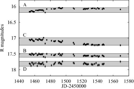
Figure 2: The R band photometry of Q2237+0305 from the GLITP collaboration. The observing period was from October 1st, 1999 (JD 2459452) to February 3th, 2000 (JD 2459577) with the Nordic Optical Telescope at Canary Islands, Spain (details in Alcalde et al. 2002). The components are labeled from A to D (Yee 1988). The bands indicate the amplitude of each component and are defined by the maximum and the minimum magnitude in each lightcurve. The widths of these bands are $\Delta m_{A}=0.154$ mag, $\Delta m_{B}=0.116$ mag, $\Delta m_{C}=0.238$ mag and $\Delta m_{D}=0.155$ mag.

For a given component, we define the largest fluctuation in the lightcurve by the difference between the maximum and the minimum magnitudes. Thus $\Delta m_{X}=|m_{X,max}-m_{X,min}|$, where X denotes component A, B, C or D. For the simulated microlensing lightcurves the condition to be fulfilled then is: $\Delta m_{X}(simul)\leq\Delta m_{X}$, where $\Delta m_{X}(simul)$ is the difference between the maximum and the minimum in the simulated lightcurve (again X stands for the four components A, B, C or D). In this way, for each set of simulations, if at least one component shows fluctuations larger than observed, then the set is rejected. For component A we obtained $\Delta m_{A}=0.154$ mag; for component B, $\Delta m_{B}=0.116$ mag; for component C, $\Delta m_{C}=0.238$ mag and for component D, $\Delta m_{D}=0.155$ mag (see Fig. 2).

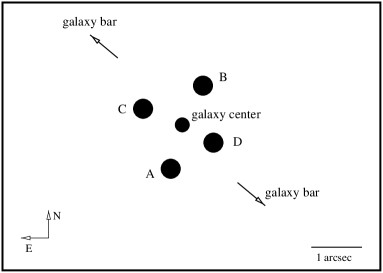
Figure 3: Relative positions of the quasar images, galaxy center and galaxy bar. The direction of motion relative to the external shear is not independent between the images because of the cross-like configurations. Thus, this is orthogonal between images A$\perp$C and B$\perp$D, whereas the direction for image A is parallel to the one in image B, and similarly for images C and D.

It is important to notice that if erronous outliers would be present in the photometry, the result would be an overestimate: the largest actual fluctuations would be lower than the obtained result. This would result in a larger upper limit on the transverse velocity, hence the approach we use is conservative. However, looking at Figure 2, this seems an unlikely possibility.

3.3 Microlensing Simulations

We computed magnification patterns for the four quasar images, using the Schmidt et al. (1998) model for the values of $\kappa$ and $\gamma$ (cf. Table 1). We assumed all compact objects have the same mass, $M_{\rm\mu lens}$ (realistic mass functions act roughly as their respective mass averages, so we take $M_{\rm\mu lens}=0.1M_{\odot}$ and $M_{\rm\mu lens}=1M_{\odot}$ as extreme cases; see i.e. Lewis & Irwin 1995). The physical side lengths of these maps were $15\leavevmode\nobreak\ r_{E}$ covered by $4500$ pixels, resulting in a spatial resolution of 300 pixels per Einstein radius $r_{E}$. For each component we did a number of different random realizations of maps of this size, to be sure that they were statistically representatives. The effect of the finite source size is included by convolving the magnification patterns with a certain source profile. We adopted a Gaussian surface brightness profile for the quasar with three different values of the width $\sigma_{Q}$= $0.003$ $r_{E}$, $0.01$ $r_{E}$ and $0.05$ $r_{E}$. This corresponds to physical effective radii from $2\times 10^{14}$ cm to $3\times 10^{15}$ cm for $M_{\rm\mu lens}=0.1M_{\odot}$, and a factor of $\sqrt{10}$ larger for lens masses of $M_{\rm\mu lens}=1.0M_{\odot}$. Much larger source sizes are excluded by the large amplitude fluctuations in this system observed by Woźniak et al. (2000a,b), as was shown by Yonehara (2001) and Wyithe, Webster & Turner (2000a). Therefore we can restrict our analysis to small source sizes. In addition, we remark that the important contribution of the source in our simulations comes from its scale and more realistic models for the source are considered second order effects. This can be better understood if we think that ’fine structure’ of these realistic models will produce refined fluctuations in the simulated lightcurves. But this fluctuations are originated close to caustics and the method is based on the selection of realizations with low fluctuations, where this ’fine structure’ does not exist.

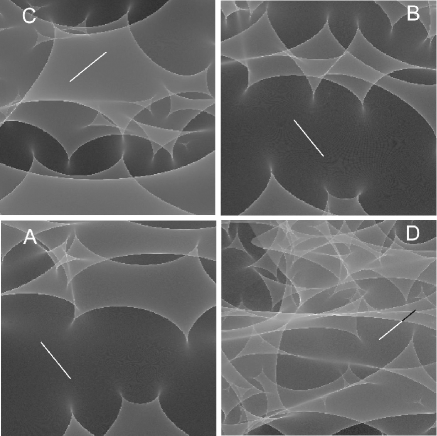
Figure 4: A part of the total magnification pattern for each component, labeled and ordered as in Fig. 3. The length of the white part of the track is determined in such a way as to fulfill the criterion $\Delta m_{X}(simul)\leq\Delta m_{X}$, where $X$ denotes the component A, B, C or D. The black part of the track in component D introduces variability higher than the observed one, making this set not compatible with the observations.

In order to statistically infer an upper limit on the permitted length of the linear tracks across the magnification maps, we do the following (for a given source size): we first fix the length of the track and randomly select a starting pixel in the magnification pattern of one of the images, say component A. Then we select a random direction for which the magnification along a linear track is going to be computed. As the next step, random starting points in the magnification patterns of the other images are selected. However, this time the direction is not arbitrary: The direction of motion in all the images relative to the external shear is fixed, the displacements of the source in the magnification maps B, C and D are no longer independent. In fact, because of the cross-like geometrical configuration of the system, A and B are parallel to each other, as are C and D. These two pairs are orthogonal relative to each other: A$\perp$C and B$\perp$D (cf. Fig. 3 motivated by Fig. 1 in Witt and Mao, 1994). Thus, once the direction in the magnification pattern A is selected, the ones in the magnification patterns B, C, and D are determined as well. So in this way we construct simultanously sets of test lightcurves for the four quasar images along linear tracks for a given track length. This is illustrated in Fig. 4, where a small part of each of these magnification patterns is shown (side length is $L\approx 4\leavevmode\nobreak\ r_{E}$). White color indicates high magnification while black means low magnification. The linear tracks drawn inside the maps in Fig. 4 illustrate the calculation procedure.

When $\Delta m_{X}(simul)$ – the amplitudes between maximum and minimum of the simulated lightcurves for images A, B, C, and D – are larger than $\Delta m_{X}$, then this particular set of lightcurves is marked as not compatible with the observations. In the example shown in Fig. 4, the parts of the four tracks with amplitudes lower than the observed ones corresponds to the white part.

This procedure is performed for 50000 sets of tracks/lightcurves per given track length, and repeated it for different lengths, ranging from $0.01\leavevmode\nobreak\ r_{E}$ to $1\leavevmode\nobreak\ r_{E}$ in steps of $0.003\leavevmode\nobreak\ r_{E}$ (which numerically corresponds to lengths of $3$ to $300$ pixels in steps of one pixel). This corresponds to a total of $1.5\times 10^{7}$ simulated tracks. For each considered track length, we determine then the fraction of tracks not compatible with the observations, i.e., the probability distribution.

From this distribution we can now derive $l_{\rm upper}$ from the probability $P(l\leq l_{\rm upper})$ = 90%, i.e., the 90 per cent upper limit on the allowed path lengths (or similarly, the 68% or 95% levels). The whole procedure was repeated for magnification patterns constructed with the $\kappa$ and $\gamma$ values of the Schneider et al. (1988) model, see Table 1. The results (presented in the next section) were indistinguishable.

4 Results

The resulting probability distributions for the fraction of lightcurves which showed more fluctuations than the observed ones are shown in Fig. 5 for each track length in units of Einstein radii. The three curves represent the three different source sizes we considered: $\sigma_{Q}=0.003\leavevmode\nobreak\ r_{E}$ (thin line), $\sigma_{Q}=0.01\leavevmode\nobreak\ r_{E}$ (medium line) and $\sigma_{Q}=0.05\leavevmode\nobreak\ r_{E}$ (thick line).

Figure 5: Probability distribution for the fraction of light curves with a given length which produce larger fluctuations than what is observed. We consider three different source sizes: $\sigma_{Q}=0.003\leavevmode\nobreak\ r_{E}$ (thin line), $\sigma_{Q}=0.01\leavevmode\nobreak\ r_{E}$ (medium line), and $\sigma_{Q}=0.05\leavevmode\nobreak\ r_{E}$ (thick line). Horizontal dotted lines indicate the different cuts in percentages, corresponding to the values listed in Table 2.

From each distribution we can determine the upper limit on the length of the tracks consistent with the variability of the observed lightcurves defined by the bands described before. The values are given in Table 2 for three different “confidence levels” of 68%, 90% and 95%, for the three source sizes used. We estimate the uncertainty in $l_{upper}$(90%) from the $\sqrt{N}$ statistics, where $N$ is the number of simulations at the 90% point: The error is $\pm 0.02\leavevmode\nobreak\ r_{E}$. The results are almost independent of the source size (within the considered range), as is apparent from Figure 5 as well. This is not too surprising, because in a “flat” part of the magnification pattern, where most of our simulations will take place, a large source is (de-)magnified by the same amount as a small source (in the considered range of source sizes, the length of the tracks is always much larger than the size of the source). Only when a caustic is approached, this changes.

C.L.	source sizes
	$\sigma_{Q}=0.003\leavevmode\nobreak\ r_{E}$	$\sigma_{Q}=0.01\leavevmode\nobreak\ r_{E}$	$\sigma_{Q}=0.05\leavevmode\nobreak\ r_{E}$
68%	0.06 rE	0.06 rE	0.07 rE
90%	0.13 rE	0.13 rE	0.13 rE
95%	0.17 rE	0.18 rE	0.18 rE

Table 2: Results for the length of the simulated tracks $l_{\mathrm{u}pper}$ as a function of source size for different confidence levels; at the 90% the uncertainty is $\pm 0.02\leavevmode\nobreak\ r_{E}$.

These track lengths can be converted into physical quantities by using Eq. 2 and a given value for the mass of the microlenses, $M_{\rm\mu lens}$. As we are observing the inner part of the lens galaxy with presumably an old stellar population, a resonable range for the microlens mass is $0.1M_{\odot}\leq M_{\rm\mu lens}\leq 1M_{\odot}$ (Alcock et al. 1997, Lewis & Irwin 1995, Wyithe et al. 2000a). Using the length of the observing interval, $t_{\rm obs}=126$ days, we can deduce $v_{\rm upper}$, the upper limit on the effective tranverse velocity in this lens system.

In calculating the effective transverse velocity of the lens in the lens plane from these numbers, we need to use the following expression (Kayser et al. 1986):

$$\@vec{V}=\frac{1}{1+z_{s}}\leavevmode\nobreak\ \@vec{v_{s}}-\frac{1}{1+z_{d}}\frac{D_{s}}{D_{d}}\leavevmode\nobreak\ \@vec{v_{d}}+\frac{1}{1+z_{d}}\frac{D_{ds}}{D_{d}}\leavevmode\nobreak\ \@vec{v_{obs}}$$ (3)

where $\@vec{V}$ is the effective transverse velocity of the system, $\@vec{v_{s}}$ the velocity of the source, $\@vec{v_{d}}$ the velocity of the deflector (lens), and $\@vec{v_{\rm obs}}$ the velocity of the observer. The effective transverse motion of the lens includes the true transverse velocity of the galaxy as a whole and an effective contribution due to the stellar proper motions. For the adopted concordance cosmology ($\Omega_{o}=0.3$, $\Lambda_{o}=0.7$ and $H_{0}=65$ km sec^-1 Mpc^-1) and the redshifts of the source and deflector, $z_{s}$ and $z_{d}$, respectively, Equation 3 can be evaluated to get:

$${V}=0.37\leavevmode\nobreak\ {v_{s}}-10.55\leavevmode\nobreak\ {v_{d}}+10.18\leavevmode\nobreak\ {v_{\rm obs}}.$$ (4)

Comparison of the Earth’s motion relative to the microwave background (Lineweaver et al. 1996) with the direction to the quasar Q2237+0305 indicates that these vectors are almost parallel, so that the last term on the right hand side of Eq. 4 can be neglected: the transverse part is very small (in fact  $v_{\rm obs}\simeq 50$ km sec^-1, and this value can in general be known from the dipole term in the microwave background radiation and the direction towards the lens in any gravitational lens system). Furthermore, assuming that the peculiar velocities of the quasar and the lensing galaxy, ${v_{s}}$ and ${v_{d}}$, are of the same order, the first term can be neglected as well, since its weight is only about $4\%$ of the total. In this way, we just keep the expression

$${V}\leavevmode\nobreak\ \simeq\leavevmode\nobreak\ 10.55\leavevmode\nobreak\ {v_{d}}.$$ (5)

An upper limit for the effective transverse velocity of the lens in the lens plane, ${v_{d}}$, can now be calculated by just setting ${V}=V_{\rm upper}$. Here we assumed $V_{\rm upper}$ to be the 90% limit on the effective transverse velocity, i.e. it is based on the 90% length $l_{\mathrm{u}pper}=0.13\leavevmode\nobreak\ r_{E}$, as inferred from the simulations. The resulting value for the 90%-limit on the transverse velocity of the lensing galaxy obtained in this way depends on the assumed mass of the microlenses (and is independent of the quasar size). For $M_{\rm\mu lens}=0.1M_{\odot}$, we obtain:

$${v_{d,0.1M_{\odot},90\%}}\leq 685\leavevmode\nobreak\ {\rm km/s}$$

for all the source sizes considered. The limits for masses of $M_{\rm\mu lens}=1.0M_{\odot}$ is

$${v_{d,1.0M_{\odot},90\%}}\leq 2175\leavevmode\nobreak\ {\rm km/s}.$$

It is even possible to place slightly stronger limits on ${v_{\rm bulk}}$. The reason is that the actual effective lens velocity ${v_{d}}$ is a combination of the bulk velocity of the galaxy as a whole (${v_{\rm bulk}}$) and the velocity dispersion of the microlenses (${v_{\rm\mu lens}}$). This latter effect was studied by Schramm et al. (1992), Wambsganss & Kundic (1993) and Kundić & Wambsganss (1995), and it was found that the two velocity contributions combined are producing the effective velocity in the following way:

$${v_{d}}=\sqrt{{v_{\rm bulk}}^{2}+(a\leavevmode\nobreak\ {v_{\rm\mu lens}})^{2}}$$ (6)

where $a$ represents the effectiveness of microlensing produced by the velocity dispersion versus the bulk motion. As the velocity dispersion of compact objects is more or less a random motion, the parameter $a$ is independent of the tranverse motion of the bulk. The value of this ‘effectiveness parameter’ is $a\leavevmode\nobreak\ \approx\leavevmode\nobreak\ 1.3$ (see Wambsganss & Kundic 1993, Kundić & Wambsganss 1995 for details). Since the central velocity dispersion of the lensing galaxy in Q2237+0305 has been measured: ${v_{\rm\mu lens}}\leavevmode\nobreak\ \simeq\leavevmode\nobreak\ 215$ km/s (Foltz et al. 1992), we can use that and infer an even lower value for the upper limit on the effective velocity of the bulk motion (the velocity dispersion at the location of the images could be slightly different, though):

$${v_{\rm bulk,0.1\leavevmode\nobreak\ M_{\odot},90\%}}\leavevmode\nobreak\ \leq\leavevmode\nobreak\ 625\leavevmode\nobreak\ {\rm km/s}\ \ {\rm for}\ \ M_{\rm\mu lens}=0.1M_{\odot}$$

and

$${v_{\rm bulk,1.1\leavevmode\nobreak\ M_{\odot},90\%}}\leavevmode\nobreak\ \leq\leavevmode\nobreak\ 2157\leavevmode\nobreak\ {\rm km/s}\ \ {\rm for}\ \ M_{\rm\mu lens}=1.0M_{\odot}.$$

5 Discussion

Wyithe et al. (1999) presented the first determination of the effective transverse velocity of the lens galaxy in Q2237 via microlensing. Here we compare this approach to ours. First, the Wyithe et al. method uses a number of microlensing events, with a base monitoring line of the order of 10 years or so. Our method – based on the amplitude of observed lightcurves – can be applied to shorter monitoring base lines (typically one order of magnitude lower) and is more restrictive in the absence of microlensing fluctuations. In principle, in the absence of microlensing events, both methods should yield similar results. Second, our statistics is simple and straighforward: fluctuations higher than the observations are ruled out in the simulations, no other assumptions are necessary. Third, our method is source size independent in the considered range. The Wyithe et al. results are slightly dependent on the source size, although their largest upper limit is obtained for a point source (see their Fig. 12). On the other hand, Wyithe et al. constrain both mass and velocity simultanously, whereas in our case we assume we have some information on the mass range.

More recently, Kochanek (2004) developed a general method for analyzing microlensed quasar lightcurves, trying to simultaneously fit the effective source velocity, the average stellar mass, the stellar mass function and the size and structure of the quasar accretion disk. This ambitious task is performed by a multidimensional $\chi^{2}$ statistic with an enormous computational effort, but considers more realistic quasar models. Our calculations for the effective transverse velocity are computationaly cheap and easily applicable to other systems.

The result we adopt for the upper limit of the effective transverse velocity of the lens galaxy (${v_{\rm bulk}}\leavevmode\nobreak\ \leq\leavevmode\nobreak\ 630$ km/s, 90% c.l., considering $M_{\rm\mu lens}=0.1M_{\odot}$) is slightly higher than that obtained by Wyithe et al. (${v_{\rm bulk}}\leavevmode\nobreak\ \leq\leavevmode\nobreak\ 500$ km/s at a 95% c.l.) but lower than that reported by Kochanek (2004) (${v_{\rm bulk}}\leavevmode\nobreak\ \leq\leavevmode\nobreak\ 1800$ km/s, 68% c.l, for $M_{\rm\mu lens}=0.1M_{\odot}$). Kochanek (2004) remarked that the significant variability of the quasar during the OGLE monitoring period (he analyzed the $V$-band OGLE data set) may be the cause of the relatively high velocities found in his work.

6 Conclusions

Estimating peculiar motions of galaxies is in general a difficult task. We have here derived upper limits to the transverse velocity of the lensing galaxy in the quadruple quasar system Q2237$+$0305, using four months of monitoring data from the GLITP collaboration (Alcalde et al. 2002). Although we took the amplitude limits from all the lightcurves, the results are mainly constrained by components B and D, where no strong microlensing signals are present. The idea of the method is simple and straightforward: if the galaxy is moving through the network of microcaustics and no or little microlensing is present in the observations, this defines a typical length of the low magnification regions in the magnification patterns, which in turn can be converted into a physical velocity, when the length of the observing interval is considered.

This typical length is derived in a statistical sense from intensive numerical simulations using two different macro models for the lens (which both produce the same results). The resulting value obtained for this upper limit on the transverse velocity of the lensing galaxy is $v_{\rm bulk,0.1M_{\odot},90\%}\leq 630$ km/s for lens masses of $M_{\rm\mu lens}=0.1M_{\odot}$ and $v_{\rm bulk,1.0M_{\odot},90\%}\leq 2160$ km/s for lens masses of $M_{\rm\mu lens}=1.0M_{\odot}$. Within the error estimation for this limit, the result is independent of the quasar sizes considered (Gaussian width from 0.003 r_E to 0.05 r_E, which corresponds to the range of $2\times 10^{4}$ cm to $3\times 10^{5}$ cm, in the case of $M_{\rm\mu lens}=0.1M_{\odot}$). Future monitoring campaigns of this and other multiply imaged quasars can be used to provide more and stronger limits on the transverse velocities of lensing galaxies, in particular using quiet periods in systems where microlensing has been previously detected.