Cosmic homogeneity demonstrated with luminous red galaxies

Abstract

We test the homogeneity of the Universe at $z\sim 0.3$ with the Luminous Red Galaxy (LRG) spectroscopic sample of the Sloan Digital Sky Survey. First, the mean number $N(R)$ of LRGs within completely surveyed LRG-centered spheres of comoving radius $R$ is shown to be proportional to $R^{3}$ at radii greater than $R\sim 70\,h^{-1}~{}\mathrm{Mpc}$. The test has the virtue that it does not rely on the assumption that the LRG sample has a finite mean density; its results show, however, that there is such a mean density. Secondly, the survey sky area is divided into 10 disjoint solid angular regions and the fractional rms density variations of the LRG sample in the redshift range $0.2<z<0.35$ among these ($\sim 2\times 10^{7}\,h^{-3}~{}\mathrm{Mpc^{3}}$) regions is found to be 7 percent of the mean density. This variance is consistent with typical biased $\Lambda$CDM models and puts very strong constraints on the quality of SDSS photometric calibration.

1 Introduction

One of the principal assumptions of successful physical cosmological models is homogeneity; i.e., the assumption that sufficiently large independent volumes of the Universe will contain similar mean densities of matter (and everything else). In detail, any test of this assumption becomes a quantitative one: Do the observed variations of density agree with the predictions of the leading physical theories? Inasmuch as astronomical observations are used to rule out physical theories, the homogeneity of the Universe cannot be demonstrated definitively beyond this. This is not because the observations suggest an inhomogeneous Universe, but rather because there are no physical inhomogeneous models to rule out!

In fact the observations do strongly suggest homogeneity, and the great success of the $\Lambda$CDM model in explaining the statistical fluctuations in the isotropic cosmic microwave background (CMB; e.g., Bennett et al., 2003), the growth of present-day large-scale structure (e.g., Tegmark et al., 2004), and the tight redshift-distance relation inferred for type Ia supernovae (Schmidt et al., 1998; Perlmutter et al., 1999) should be taken as very strong evidence that the Universe is homogeneous on large scales. It does not make sense to postulate inhomogeneous matter distributions without providing a physical model in which such distributions are consistent with modern observations.

Nevertheless, in what follows we use the enormous Luminous Red Galaxy (LRG) sample (Eisenstein et al., 2001) of the Sloan Digital Sky Survey (SDSS; York et al., 2000) to test the homogeneity of the Universe with the most conservative statistical tests we know. We may not have physical inhomogeneous models to test, but such models may exist in the future, and homogeneity on large scales is an extremely strong prediction of $\Lambda$CDM and its variants. Even if homogeneity of the matter distribution is taken for granted, homogeneity in the galaxy distribution is not guaranteed if there are, e.g., factors contributing to galaxy formation that act over large distances. For these reasons, cosmic homogeneity is worthy of study.

Certainly the prevailing view in modern cosmology is that homogeneity has been very well established by the observed isotropy of the CMB (Partridge & Wilkinson, 1967; Wilson & Penzias, 1967; Smoot et al., 1992; Bennett et al., 2003), x-ray background (e.g., Scharf et al., 2000), and the isotropies of various source populations, e.g., radio galaxies (Peebles, 1993). In the context of physical models in which the CMB is emitted during recombination at early times, its isotropy is indeed a very strong argument for homogeneity. However it is certainly possible to imagine inhomogeneous distributions of finite-sized (redshift-dependent) blackbody sources such that every line of sight happens to terminate on the surface of one of them. In other words, isotropy does not by itself guarantee homogeneity. The fundamental issue is that homogeneity is a property of distributions in three-dimensional space and isotropy is a property of distributions on a two-dimensional sky.

Isotropy of a population of discrete sources merits additional discussion. As with the CMB, the isotropy of the point distribution itself does not guarantee homogeneity, as there can in principle be inhomogeneous three-dimensional distributions that project to isotropic distributions on the sky at high probability for typical observers (Durrer et al., 1997). However, we do expect that isotropy of such discrete populations provides strong evidence for homogeneity when combined with the observation that flux and redshift distributions are similar in different directions. Isotropy itself is a two-dimensional test and therefore not sufficient, but isotropy as a function of flux or redshift is indeed a three-dimensional test and probably does establish homogeneity, although at lower precision than the tests we perform below. Of course these statements (or their contraries) are hard to maintain with great confidence in the absence of any inhomogeneous physical model.

By far the cleanest tests of homogeneity involve simply counting sources in three dimensional regions. Homogeneity is established—in principle—when the three-space correlation function of galaxies can be shown to vanish over a range of scales at large scales. Unfortunately, most investigations of the correlation function use the largest scales available in the survey under analysis to determine the mean density (sometimes with an integral constraint correction). The estimation of clustering statistics involves subtraction of the mean density, so it is in some sense required by the methodology that the clustering tends to zero at the largest available scales. Indeed, it has sometimes been the case that clustering amplitudes have been underestimated in small surveys. For these reasons the vanishing of the correlation function only establishes homogeneity if it is shown to vanish over a substantial range of scales, e.g., as it has been shown to do for optically selected QSOs on scales of 100 to $2000\,h^{-1}~{}\mathrm{Mpc}$ (Croom et al., 2004).

The Sloan Digital Sky Survey Luminous Red Galaxy sample is ideal for performing these tests in an extremely conservative manner. The sample used here fills a huge volume ($\sim 0.6\,h^{-3}~{}\mathrm{Gpc^{3}}$) with high spectroscopic completeness. It contains only galaxies of a limited range of luminosities and it is close to volume-limited (Eisenstein et al., 2001). The sample contains large numbers; there are 55,000 used below. The SDSS footprint also has a good angular shape for this project; we show below that the LRG sample contains many independent filled spheres of comoving radius $R>100\,h^{-1}~{}\mathrm{Mpc}$. Previous work on cosmic homogeneity, some of which has concluded that there is evidence for a fractal-like galaxy distribution (Sylos Labini et al., 1998; Joyce et al., 1999a), have not had samples that have measured such large scales so cleanly.

In what follows, a cosmological world model with $(\Omega_{\mathrm{M}},\Omega_{\mathrm{\Lambda}})=(0.3,0.7)$ is adopted, and the Hubble constant is parameterized $H_{0}=100\,h~{}\mathrm{km\,s^{-1}\,Mpc^{-1}}$, for the purposes of calculating distances(e.g., Hogg, 1999).

2 The LRG sample

The SDSS (York et al., 2000; Stoughton et al., 2002; Abazajian et al., 2003, 2004) is conducting an imaging survey of $10^{4}$ square degrees in 5 bandpasses $u$, $g$, $r$, $i$, and $z$ (Fukugita et al., 1996; Gunn et al., 1998). Photometric monitoring (Hogg et al., 2001), image processing (Lupton et al., 2001; Stoughton et al., 2002; Pier et al., 2003), and good photometric calibration (Smith, Tucker et al., 2002) allow one to select galaxies (Strauss et al., 2002; Eisenstein et al., 2001), quasars (Richards et al., 2002), and stars for follow-up spectroscopy with twin fiber-fed double-spectrographs. The spectra cover 3800Å to 9200Å with a resolution of 1800. Targets are assigned to plug plates with a tiling algorithm that ensures nearly complete samples (Blanton et al., 2003).

We focus here on the luminous red galaxy spectroscopic sample (Eisenstein et al., 2001). This uses color-magnitude cuts in $g$, $r$, and $i$ to select galaxies that are likely to be luminous early-type galaxies at redshifts between 0.15 and 0.5. The selection is highly efficient and the redshift success rate is excellent. The sample is constructed so as to be close to volume-limited up to $z=0.36$, with a dropoff in density towards $z=0.5$. The comoving number density of the sample is close to that required to maximize the signal-to-noise ratio on the large-scale power spectrum.

The sample we use here is drawn from NYU LSS sample14 (Blanton et al., 2004) and covers 3,836 square degrees containing 55,000 LRGs between redshift of 0.16 and 0.47. We use an absolute $g$-band magnitude cut of $-21.2$, including $k$-corrections and evolution to $z=0.3$. The details of the radial and angular selection functions are described in Zehavi et al. (2004). The radial modeling of the expected number of galaxies as a function of redshift is based closely on the observed distribution. The exact survey geometry is expressed in terms of spherical polygons. We exclude the few regions that have less than 48 percent spectroscopy coverage. We weight all of our counts by the inverse of the angular selection function, including an explicit correction for fiber collisions, to bring the weighted LRG catalog to a uniform mean angular density within the chosen sky region.

We create large catalogs of randomly distributed points based on these angular and radial models. These catalogs match the distribution of the LRGs in redshift and are isotropic within the survey region. These catalogs allow us to check the survey completeness of any given volume and provide a homogeneous baseline (e.g., expected numbers) for the tests that follow.

The LRG sample depends considerably on the photometric uniformity of the SDSS. Photometric calibration is involved at two different stages in this work: The first stage is at initial target selection, because the LRG spectroscopic targets are selected on the imaging photometry, calibrated via the Photometric Telescope (Smith, Tucker et al., 2002). An 0.01 mag shift in $(r-i)$ color or a 0.03 mag shift in $r$ magnitude would modulate the LRG target density by up to 10 percent at most redshifts (Eisenstein et al., 2001). The second stage comes when the spectroscopic LRG sample is “cut down” to the volume limited sample used here by an additional absolute magnitude cut. This cut is based on improved calibration (using survey scan stripe overlap regions). The sample density is very sensitive to small shifts in calibration at this stage also.

The homogeneity that we find below is a testament to the calibration of the survey. It appears that while the survey may have small regions or even scan stripes that are miscalibrated (at $\sim 2$ percent rms), the large-scale photometric homogeneity is better than 1 percent in $(r-i)$ color, i.e., the errors average down on large scales. At no point is the uniformity of the LRG sample assumed or used in setting calibration or calibration parameters.

3 Conditioned density scaling

The fundamental test of the homogeneity of a point set, which makes no assumption about even the existence of a mean density, is the measurement of the scaling of the average number of neighboring points to any given point, as a function of maximum separation (Pietronero et al., 1987; Gabrielli et al., 2004). In a homogenous distribution, at large enough distances, this number $N$ scales with the maximum distance $R$ as $R^{D}$, where $D$ is the dimensionality of the space.

Because our goal is to be extremely conservative, for this test, we considered neighbors not of all LRGs, but only of those “target” LRGs in the redshift range $0.20<z<0.40$ that have enormous spherical comoving regions around them that have been completely surveyed by the SDSS spectroscopic survey. In detail, we required that both the $50$ and the $100\,h^{-1}$ Mpc radius comoving sphere around each target galaxy to be at least 95 percent complete (in the sense of 95 percent coverage by the spectroscopic survey, which itself is complete at the 94 percent level for LRGs). The sky distribution of the 3658 LRGs that satisfy this highly restrictive selection are shown in Figure 1.

In Figure 2 the scaling of the average number $N$ of neighbors of the target galaxies as a function of radius $R$ is shown, with an “expected number” divided out. The expected number is estimated by counting the number of “random” points in the spherical volume, where the random points are from a homogeneous random catalog described above with the same footprint, angular variation of completeness, and radial selection function as the LRGs, but 100 times the total number. Since the sample being used is highly complete, this is essentially equivalent to dividing all the counts by a constant times $R^{3}$. Figure 2 shows that the mean number $N$ scales as $R^{3}$ at large distances (and $R^{2}$ at small distances).

Also shown in Figure 2 is the average number for each of five samples, split by RA by the RA lines shown in Figure 1. Each of the five sky regions shows the $R^{3}$ scaling individually. The expected number densities from the random catalogs has been kept constant across all regions. This test is particularly conservative, because the five sky regions contain (mostly) independent spheres and are expected to have different observing and calibration properties.

4 Density variation

In an inhomogeneous universe (absent a physical inhomogeneous model), the natural expectation is for order unity differences in population densities on all scales. For this reason we performed a test in which the sky is split into disjoint regions and the number density of LRGs is tested in a comoving volume in each of the disjoint regions.

Figure 3 shows the redshift $0.20<z<0.35$ LRG sample split into 10 disjoint sky regions, each of which is of comparable total solid angle and therefore (for this redshift range) comoving volume. Each region corresponds to a comoving volume of roughly $2.2\times 10^{7}\,h^{-3}~{}\mathrm{Mpc^{3}}$. Figure 4 shows the relative densities of these regions. The rms scatter between the 10 regions is 7.3 percent. Subtracting the expected Poisson variation among these regions yields a relative rms scatter of 7.0 percent.

In a $\Lambda$CDM model with $\sigma_{8}=0.85$, the mass density fluctuations among this set of sky regions in the redshift range $0.20<z<0.35$ is expected to be 3.1 percent. The LRG real-space autocorrelation has been measured to have an amplitude $\sigma_{8}=1.80$ (Zehavi et al., 2004), so that the galaxies have a bias of around 2, and one would predict a variation of roughly 6.5 percent. Hence, the 7.0 percent variance in the LRG sample does not leave much room for calibration errors, which ought to come in in quadrature. For the LRG sample, 1 percent calibration variations in the $r-i$ color or 3 percent variations in the $r$ flux would produce $\sim 10$ percent variations in the LRG number density (Eisenstein et al., 2001), so the consistency of this measurement with the biased CDM description of the LRG population puts extremely strong constraints on the quality of SDSS photometric calibration. Note that the LRG target selection is never used to tune the photometric calibration, so there is no sense in which this uniformity is enforced directly.

5 Discussion

The extremely large (in both volume and number) and complete LRG sample from the SDSS was used to test the three-dimensional homogeneity (i.e., not just isotropy) of the Universe at $z\sim 0.3$ by the most conservative possible method. We find that the Universe has a well-defined mean density and that it is homogeneous. Furthermore, the variations we see in the density of LRGs on large scales is consistent with the predictions of a biased $\Lambda$CDM cosmogonic model.

The number $N(R)$ of LRGs within LRG-centered spheres of comoving radius $R$ is shown to be proportional to $R^{3}$ at radii greater than $R\sim 70\,h^{-1}~{}\mathrm{Mpc}$. For this test we used not all LRGs as central LRGs, but only those in the centers of highly complete spheres, so there is no “interpolation” or “extrapolation” over unobserved regions. In the terminology of fractals, this test shows that the fractal dimension of the LRG distribution is very close to $D=3$. The test has the virtue that it does not rely on the assumption that the LRG sample has a finite mean density; its results show, however, that there is such a mean density.

The $D=3$ result presented here is in qualitative disagreement with some previous studies. There are some similar kinds of analyses of redshift surveys that show $D\approx 2$ (Sylos Labini et al., 1998; Joyce et al., 1999a), but there is no quantitative disagreement, because the most robust measurements of $D$ are generally made at scales much smaller than those measured by the LRGs here. Indeed, Figure 2 shows that $D=2$ is a remarkably good fit out to roughly $20\,h^{-1}~{}\mathrm{Mpc}$. Analyses of the ESO Slice Project, in which the scaling of the number of galaxies in the sample is measured as a function of the redshift depth to which they are counted (Scaramella et al., 1998; Joyce et al., 1999b), depend crucially on $K$ corrections, evolution, and world model.

The survey sky area was divided into 10 disjoint solid angular regions and the fractional rms density variations of the LRG sample in the redshift range $0.2<z<0.35$ among these ($\sim 2\times 10^{7}\,h^{-3}~{}\mathrm{Mpc^{3}}$) regions was found to be 7 percent of the mean density. This variance is consistent with typical biased $\Lambda$CDM models, with a bias of $\approx 2$, as is found for the LRG sample at smaller scales (Zehavi et al., 2004). This result confirms homogeneity and supports the biased $\Lambda$CDM model on the largest observable scales.

Finally, it is worthy of note that because the LRG sample selection is so sensitive to photometric calibration, these results demonstrate that the calibration of the SDSS in the $g$, $r$, and $i$ bands is consistent at the sub-percent level when averaged on angular scales of tens of degrees and larger. This is a tremendous technical achievement and recommends the LRG sample and the SDSS for making many extremely precise measurements in the future.

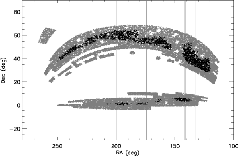
Figure 1: The entire LRG sample used in this study is shown in grey. The 3658 LRGs in the redshift range $0.2<z<0.4$ with $>95$ percent complete volumetric coverage inside the surrounding comoving spheres of radii $R=50$ and $100\,h^{-1}~{}\mathrm{Mpc}$ are shown in black. Also shown are grey lines that split the 3658 points into five quantiles by RA.

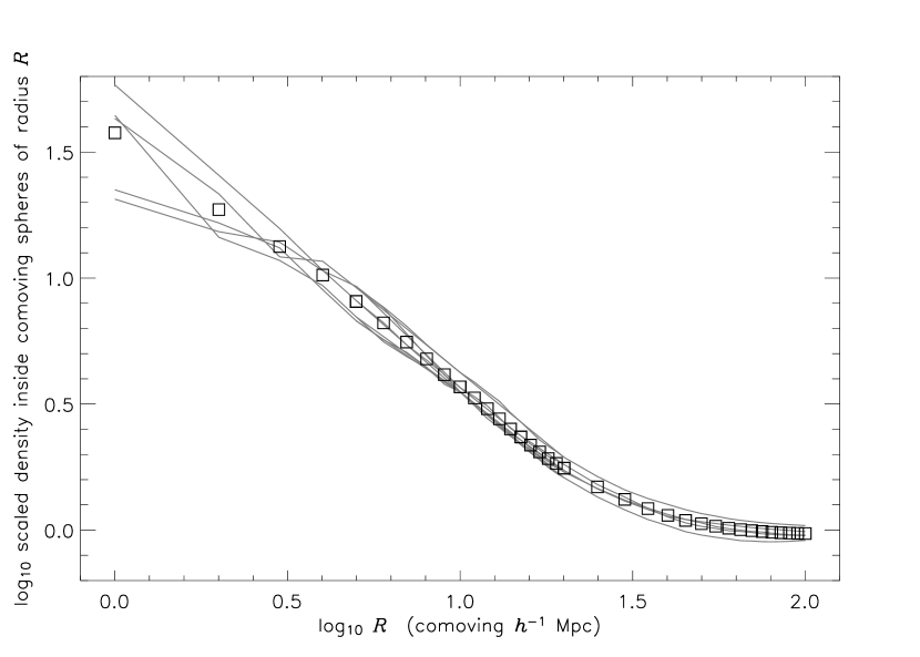
Figure 2: The average comoving number density (i.e., number counted divided by expected number from a homogeneous random catalog) of LRGs inside comoving spheres centered on the 3658 LRGs shown in Figure 1, as a function of comoving sphere radius $R$. The average over all 3658 spheres is shown in with open squares, and the averages of each of the five RA quantiles is shown as a separate grey line. At small scales, the number density drops with radius because the LRGs are clustered; at large scales the number density approaches a constant because the sample is homogeneous.

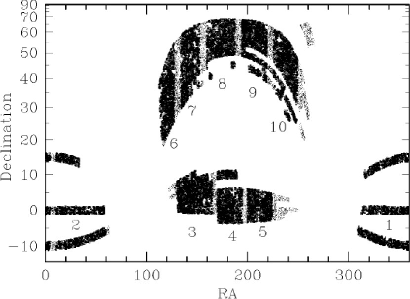
Figure 3: The LRGs in the redshift range $0.20<z<0.35$, divided into 10 disjoint sky regions (where LRGs are labeled and marked by dots and squares), with inter-region gaps (where LRGs are marked by dots only).

Figure 4: The relative comoving number densities of LRGs in the redshift range $0.20<z<0.35$ in the 10 disjoint sky areas shown in Figure 3. The quoted “$\sigma$” is the rms scatter of the points, with the expected Poisson rms subtracted out in quadrature.

References

- Abazajian et al. (2003) Abazajian, K. et al. 2003, AJ, 126, 2081
- Abazajian et al. (2004) Abazajian, K. et al. 2004, AJ, 128, 502
- Bennett et al. (2003) Bennett, C. L. et al. 2003, ApJS, 148, 1
- Blanton et al. (2001) Blanton, M. R. et al. 2001, AJ, 121, 2358
- Blanton et al. (2003) Blanton, M. R., Lin, H., Lupton, R. H., Maley, F. M., Young, N., Zehavi, I., & Loveday, J. 2003, AJ, 125, 2276
- Blanton et al. (2004) Blanton, M. R. et al. 2004, AJ, submitted
- Croom et al. (2004) Croom, S. M., Boyle, B. J., Shanks, T., Smith, R. J., Miller, L., Outram, P. J., Loaring, N. S., Hoyle, F., & da Angela, J. 2004, MNRAS, in press
- Durrer et al. (1997) Durrer, R., Eckmann, J.-P., Sylos Labini, F., Montuori, M., & Pietronero, L. 1997, Europhys. Lett., 40, 491
- Eisenstein et al. (2001) Eisenstein, D. J. et al. 2001, AJ, 122, 2267
- Fukugita et al. (1996) Fukugita, M., Ichikawa, T., Gunn, J. E., Doi, M., Shimasaku, K., & Schneider, D. P. 1996, AJ, 111, 1748
- Gabrielli et al. (2004) Gabrielli, A., Sylos Labini, F., Joyce, M., & Pietronero, L., 2004, Statistical Physics for Cosmic Structure (Springer Verlag)
- Gunn et al. (1998) Gunn, J. E., Carr, M. A., Rockosi, C. M., Sekiguchi, M., et al. 1998, AJ, 116, 3040
- Hogg (1999) Hogg, D. W. 1999, astro-ph/9905116
- Hogg et al. (2001) Hogg, D. W., Finkbeiner, D. P., Schlegel, D. J., & Gunn, J. E. 2001, AJ, 122, 2129
- Joyce et al. (1999a) Joyce, M., Montuori, M., & Sylos Labini, F. 1999a, ApJ, 514, L5
- Joyce et al. (1999b) Joyce, M., Montuori, M., Sylos Labini, F., & Pietronero, L. 1999b, A&A, 344, 387
- Lupton et al. (2001) Lupton, R. H., Gunn, J. E., Ivezić, Z., Knapp, G. R., Kent, S., & Yasuda, N. 2001, in ASP Conf. Ser. 238: Astronomical Data Analysis Software and Systems X, Vol. 10, 269
- Partridge & Wilkinson (1967) Partridge, R. B. & Wilkinson, D. T. 1967, PRL, 18, 557
- Peebles (1993) Peebles, P. J. E. 1993, Principles of physical cosmology (Princeton University Press)
- Perlmutter et al. (1999) Perlmutter, S. et al. 1999, ApJ, 517, 565
- Pier et al. (2003) Pier, J. R., Munn, J. A., Hindsley, R. B., Hennessy, G. S., Kent, S. M., Lupton, R. H., & Ivezić, Ž. 2003, AJ, 125, 1559
- Pietronero et al. (1987) Pietronero, L. 1987, Physica, 144, 257
- Richards et al. (2002) Richards, G. et al. 2002, AJ, 123, 2945
- Scaramella et al. (1998) Scaramella, R. et al. 1998, A&A, 334, 404
- Scharf et al. (2000) Scharf, C. A., Jahoda, K., Treyer, M., Lahav, O., Boldt, E., & Piran, T. 2000, ApJ, 544, 49
- Schmidt et al. (1998) Schmidt, B. P. et al. 1998, ApJ, 507, 46
- Smith, Tucker et al. (2002) Smith, J. A., Tucker, D. L., et al. 2002, AJ, 123, 2121
- Smoot et al. (1992) Smoot, G. F., et al, 1992, ApJ, 396, L1
- Stoughton et al. (2002) Stoughton, C. et al. 2002, AJ, 123, 485
- Strauss et al. (2002) Strauss, M. A. et al. 2002, AJ, 124, 1810
- Sylos Labini et al. (1998) Sylos Labini, F., Montuori, M., & Pietronero, L. 1998, Phys. Rep., 293, 61
- Tegmark et al. (2004) Tegmark, M. et al. 2004, ApJ, 606, 702
- Wilson & Penzias (1967) Wilson, R. W. & Penzias, A. A. 1967, Science, 156, 1100
- York et al. (2000) York, D. et al. 2000, AJ, 120, 1579
- Zehavi et al. (2004) Zehavi, I. et al. 2004, ApJ, submitted