Mid-infrared luminosity as an indicator of the total infrared luminosity of galaxies

The infrared (IR) emission plays a crucial role in understanding the star formation in galaxies hidden by dust. We first examined four estimators of the IR luminosity of galaxies, $L_{\rm FIR}$ (Helou et al. 1988), $L_{\rm TIR}$ (Dale et al. 2001a), revised version of $L_{\rm TIR}$ (Dale & Helou 2002) (we denote $L_{\rm TIR2}$), and $L_{\rm IR}$ (Sanders & Mirabel 1996) by using the observed SEDs of well-known galaxies. We found that $L_{\rm IR}$ provides excellent estimates of the total IR luminosity for a variety of galaxy SEDs. The performance of $L_{\rm TIR2}$ was also found to be very good. Using $L_{\rm IR}$, we then statistically analyzed the IRAS PSC$z$ galaxy sample (Saunders et al. 2000) and found useful formulae relating the MIR monochromatic luminosities [$L(12\,\mu\mbox{m})$ and $L(25\,\mu\mbox{m})$] and $L_{\rm IR}$. For this purpose we constructed a subsample of 1420 galaxies with all four IRAS band (12, 25, 60, and $100\,\mu$m) flux densities. We found linear relations between $L_{\rm IR}$ and MIR luminosities, $L(12\,\mu\mbox{m})$ and $L(25\,\mu\mbox{m})$. The prediction error with a 95 % confidence level is a factor of 4–5. Hence, these formulae are useful for the estimation of the total IR luminosity only from $12\,\mu$m or $25\,\mu$m observations. We further tried to make an ‘interpolation’ formula for galaxies at $0<z<1$. For this purpose we construct the formula of the relation between 15-$\mu$m luminosity and the total IR luminosity. We conclude that the 15-$\mu$m formula can be used as an estimator of the total IR luminosity from $24\,\mu$m observation of galaxies at $z\simeq 0.6$.

1 Introduction

Star formation activity is one of the fundamental properties useful to explore the evolution of galaxies in the universe. Generally, the star formation rate is measured by the emission from young stars, i.e., ultraviolet (UV) and related nebular line emissions. However, a significant fraction of UV photons are absorbed and re-emitted by dust mainly in the infrared (IR), hence the IR emission plays a crucial role for an understanding of the obscured star formation in galaxies (e.g., Buat et al. 1999, 2002; Hirashita et al.2003).

Further, clarifying the correlation between flux densities at various IR bands is an important task to understand the origin, release and transfer of energy in galaxies. Such studies play a crucial role in constructing and verifying IR galaxy evolution models (e.g., Granato et al. 2000; Franceschini et al. 2001; Takeuchi et al. 2001a, b; Takagi et al.2003).

Based on their 12-$\mu$m sample of galaxies, Spinoglio et al. (1995) made a pioneering study to examine various correlations between flux densities from near-IR (NIR) to far-IR (FIR), and presented useful diagnostics for Seyferts and normal galaxies on color-color diagrams. They also found that the 12-$\mu$m luminosity correlates well with the bolometric ($0.4\mbox{--}300\,\mu$m) luminosity.

Now that data obtained by Spitzer have started to become available, we are better able to explore the IR properties of galaxies at high redshift. The 24-$\mu$m band of Spitzer MIPS is very sensitive (e.g., Papovich et al. 2004), and will be used extensively for the studies of high-$z$ galaxies. Hence, from a practical point of view, it is worthwhile to find a good estimation method of the total IR luminosity of galaxies from the mid-IR (MIR) luminosity. This will also be useful for forthcoming IR space missions, e.g., ASTRO-F.

In this work, we present the estimation formulae for the FIR luminosity from the MIR. We focus on the relation between MIR and total IR luminosities, in contrast to Spinoglio et al. (1995), who used the bolometric luminosity integrated from the optical to the IR. For this purpose, we have to rely on some conventional formulae to estimate the total IR luminosity, since direct measurement of the total IR luminosity is possible only for a limited number of galaxies. First we examine the performance of four formulae in use, using galaxies with well-measured spectral energy distributions (SEDs). This sample consists of 17 galaxies ranging from dwarfs to ultraluminous, and from cool (submillimetre bright) to hot (MIR bright) ones.

We then perform a correlation analysis for the galaxy sample extracted from IRAS PSC$z$, and obtain a statistical formula for the estimation of the total IR luminosity from MIR luminosities. This statistical sample is selected by the criterion that the galaxy has all four IRAS flux density values. By combining the formula and ISOCAM 15-$\mu$m data, we then give an interpolation formula of the FIR luminosity for galaxies at $z\simeq 0.6$ observed in the Spitzer MIPS 24-$\mu$m band.

The paper is organized as follows: we examine the four estimators of the total IR luminosity in Sect. 2. We present our statistical analysis based on IRAS PSC$z$ galaxies in Sect. 3. A reexamination of the estimator $L_{\rm IR}$ and application to galaxies at $z\simeq 0.6$ are given in Sect. 4. Sect. 5 is devoted to our conclusions. The SEDs of observed galaxies used in Sect. 2 are shown in Appendix A. Mathematical details of the regression analysis are presented in Appendix B.

We denote the flux densities at a wavelength $\lambda$ by a symbol $S_{\lambda}$, but the unit is [Jy]. Throughout this work, we assume a flat lambda-dominated low-density universe with cosmological parameter set $(h,\Omega_{0},\lambda_{0})=(0.7,0.3,0.7)$, where $h=H_{0}/100\;[\mbox{km\,s}^{-1}\mbox{Mpc}^{-1}]$.

2 Performance of the estimators for the total IR luminosity

Table 1: Well-known galaxy sample.

Name	Referencesa
Normal galaxies ($10^{9}L_{\odot}<{L_{\rm IR}^{\rm total}}^{\mathrm{b}}<10^{11}L_{\odot}$)
M 63	1
M 66	1
M 82	1
M 83	1
NGC 891	1
NGC 3079	1
NGC 4418	1
NGC 7714	1
IR luminous galaxies ($L_{\rm IR}^{\rm total}>10^{11}L_{\odot}$)
NGC 2623	1,2
NGC 7679	1,2
UGC 2982	1,2
UGC 8387	1,2
Arp~220	1,3
IRAS~F10214$+$4724	1,4
Dwarf galaxies ($L_{\rm IR}^{\rm total}<10^{9}L_{\odot}$)
NGC 1569	1,5
II~Zw~40c	1,6
SBS~0335$-$052c	1,7,8

• References: 1. NED, 2. Dunne & Eales (2001), 3. (Downes et al.1993), 4. Downes et al. (1992), 5. Galliano et al. (2003), 6. Madden (2000), and 7. Dale et al. (2001b). 8. Houck et al. (2004).

• Total IR luminosity $L_{\rm IR}^{\rm total}$ is calculated by integrating over the wavelength range of $\lambda=8\mbox{--}1000\,\mu$m.

• The longest wavelength flux densities are calculated by an extrapolation using the model of Takeuchi et al. (2003a).

Since direct measurement of the total IR luminosity is only available for a limited number of galaxies, we have to use a formula to estimate the total IR luminosity from discrete photometric data, mainly in the IRAS bands. In this section, we examine the performance of four formulae in use.

2.1 Estimators

First, we define ${\cal L}_{\nu}$ as the luminosity per unit frequency at a frequency $\nu=c/\lambda$ ($c$: the speed of light). The unit of ${\cal L}_{\nu}$ is $[\mbox{erg\,s}^{-1}\mbox{Hz}^{-1}]$ throughout this work.

We examine the following four total IR luminosity estimators.

1. The classical FIR luminosity between $\lambda=42\mbox{--}122\,\mu\mbox{m}$ (Helou et al. 1988), defined as

   $$L_{\rm FIR} \equiv 3.29\times 10^{-22}$$ (1)

   $$\times\left(2.58{\cal L}_{\nu}(60\mu\mbox{m})+{\cal L}_{\nu}(100\mu\mbox{m})\right)\;[L_{\odot}]\;.$$

2. The ‘total’ IR luminosity, TIR ($\lambda=3\mbox{--}1100\,\mu$m), advocated by Dale et al. (2001a)

   $$L_{\rm TIR}\equiv L_{\rm FIR}\times 10^{a_{0}+a_{1}x+a_{2}x^{2}+a_{3}x^{3}+a_{4}x^{4}}\;[L_{\odot}]$$ (2)

   where $x\equiv\log(S_{60}/S_{100})$, and $(a_{0},a_{1},a_{2},a_{3},a_{4})=(0.2738,-0.0282,0.7281,0.6208,0.9118)$.

3. The updated version of the TIR ($\lambda=3\mbox{--}1100\,\mu$m) presented by Dale & Helou (2002) (here we denote $L_{\rm TIR2}$)

   $$L_{\rm TIR2} \equiv 2.403 \nu{\cal L}_{\nu}(25\mu\mbox{m})-0.2454\nu{\cal L}_{\nu}(60\mu\mbox{m})$$ (3)

   $$+1.6381\nu{\cal L}_{\nu}(100\mu\mbox{m})\;[L_{\odot}].$$

   This is better calibrated for submillimeter wavelengths than $L_{\rm TIR}$.

4. The luminosity between $\lambda=8\mbox{--}1000\,\mu\mbox{m}$ presented by Sanders & Mirabel (1996). In this work we refer to their IR luminosity estimator as $L_{\rm IR}$.

   $$L_{\rm IR} \equiv 4.93\times 10^{-22}\left[13.48{\cal L}_{\nu}(12\mu\mbox{m})+5.16{\cal L}_{\nu}(25\mu\mbox{m})\right.$$ (4)

   $$+2.58{\cal L}_{\nu}(60\mu\mbox{m})+\left.{\cal L}_{\nu}(100\mu\mbox{m})\right]\;[L_{\odot}]\;.$$

2.2 Examination of the IR luminosity estimators by known galaxies

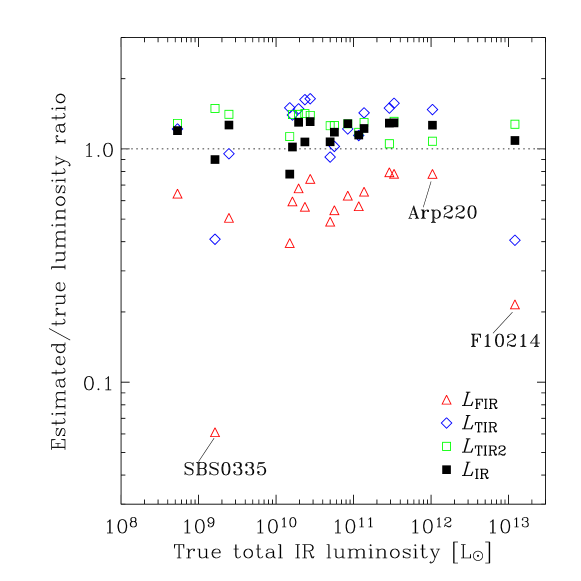
Figure 1: Comparison between the true total infrared luminosity and the estimated luminosity of galaxies. Open triangles, open diamonds, open squares and filled squares represent the ratios $L_{\rm FIR}/L_{\rm IR}^{\rm total}$, $L_{\rm TIR}/L_{\rm IR}^{\rm total}$, $L_{\rm TIR2}/L_{\rm IR}^{\rm total}$, and $L_{\rm IR}/L_{\rm IR}^{\rm total}$, respectively.

Though these IR luminosity estimators are popular in related fields, direct comparison between the measured IR luminosity and the estimated value has rarely been done to date. We examine the performance of the above estimators using the SEDs of observed galaxies. We compiled 17 galaxies with well-measured flux densities, with a total IR luminosity range of $10^{8}L_{\odot}\la L_{\rm IR}^{\rm total}\la 10^{13}L_{\odot}$ (see Table 1). Among the dwarf galaxy sample ($L_{\rm IR}^{\rm total}<10^{9}L_{\odot}$), the longest wavelength data (i.e., FIR and submm) are not available for II~Zw~40 and SBS~0335$-$052. We calculated the flux densities by extrapolating their SEDs using the model of Takeuchi et al. (2003a) (see also Takeuchi & Ishii 2004). The compiled SEDs are presented in Appendix A.

We calculated $L_{\rm IR}^{\rm total}$ by integrating the observed data directly within a wavelength range of $\lambda=8\mbox{--}1000\,\mu$m by interpolation and extrapolation. Figure 1 shows the comparison between $L_{\rm IR}^{\rm total}$ and estimated luminosities of galaxies. As expected, the classical $L_{\rm FIR}$ gives systematically lower luminosities than the true ones, because it represents the luminosity at $42\mbox{--}122\,\mu$m, and therefore the MIR and submm radiations are not included. Especially, two galaxies with hot dust (SBS~0335$-$052 and IRAS~F10214$+$4724) significantly deviate downward from the diagonal line.

Dale et al. (2001a) considered the correction factor for the contribution outside the range of $L_{\rm FIR}$ as a function of the ratio $S_{60}/S_{100}$. We see that the estimation is clearly improved, but the IR luminosities of the two extreme objects are still underestimated. This is because their $L_{\rm TIR}$ has been designed for normal galaxies, and not for such extreme objects.

In contrast to the above two estimators, $L_{\rm TIR2}$ and $L_{\rm IR}$ give much better estimates for all the galaxies in Table 1. They work not only for the objects with very hot dust emission like IRAS~F10214$+$4724 and SBS~0335$-$052, but also for a heavily extinguished galaxy like Arp~220. For SBS~0335$-$052, $L_{\rm IR}$ gives a better result. This is an expected result because $L_{\rm TIR2}$ uses three (25, 60, and $100\,\mu$m), and $L_{\rm IR}$ uses all four IRAS flux densities. In general, $L_{\rm TIR2}$ gives slightly larger values than $L_{\rm IR}$ does, probably because the considered wavelength range for the former ($\lambda=3\mbox{--}1100\,\mu$m) is wider than that for the latter ($\lambda=8\mbox{--}1000\,\mu$m).

Thus, $L_{\rm IR}$ is the best estimator of the total IR luminosity. As long as we have the four IRAS flux densities, we can obtain a precise estimate for the total IR luminosity. When data in three (25, 60 and $100\,\mu$m) or two (60 and $100\,\mu$m) bands are available, $L_{\rm TIR2}$ and $L_{\rm TIR}$ give reasonable values except for galaxies with extremely hot dust. $L_{\rm TIR2}$ works almost as accurately as $L_{\rm IR}$. In the following discussions we regard $L_{\rm IR}$ as the correct estimate of $L_{\rm IR}^{\rm total}$ and use $L_{\rm IR}$ as $L_{\rm IR}^{\rm total}$ itself.

3 Statistical analysis of the IRAS sample

Our next step is to find a conventional formula to estimate $L_{\rm IR}$ only from a single MIR band. For this purpose, we make a regression analysis for $L_{\rm IR}$ and MIR luminosities in the IRAS bands. Here we define the luminosity at a wavelength $\lambda$, $L(\lambda)$, as

$$L(\lambda)\equiv\lambda{\cal L}_{\lambda}=\nu{\cal L}_{\nu}\,,$$ (5)

and we discuss $L(12\,\mu\mbox{m})$ and $L(25\,\mu\mbox{m})$. Mathematical details of the regression analysis can be found in Appendix B.

3.1 IRAS Sample

We selected a sample from IRAS PSC$z$ (hereafter PSC$z$, Saunders et al. 2000). The PSC$z$ is a complete, flux-limited all-sky redshift survey catalog of IRAS galaxies with a detection limit of $S_{60}>0.6$ Jy. It contains 15411 IRAS galaxies with redshifts. Out of the whole sample, we selected galaxies with good quality flux densities for all four IRAS bands (12, 25, 60, and $100\,\mu$m) for this analysis, because $L_{\rm IR}$ requires all four flux densities. We performed this procedure as follows: 1. We examined the flux origin and quality flags given in PSC$z$ for the point source flux density, and omitted galaxies with upper limits (denoted as 1 in pscz.dat), 2. We extracted the coadded or extended addscan flux densities. We adopted this selection because we found that the addscan/coadded fluxes with quality flag 1 include unrealistic values close to the upper limits in point source flux densities.

There is a caveat that the selection by using all the four IRAS bands would introduce a subtle sample bias in the analysis. In order to see if the bias is serious, we also made a subsample by omitting the galaxies with flag 1 only at $100\,\mu$m (3260 galaxies included). This subsample for comparison gave essentially the same result as the above sample (the difference was less than $\sim 1\,\%$). This means that the selection in the MIR affects the result only very slightly, and the sample properties are controlled by the FIR. It is a clear contrast to the sample of Spinoglio et al. (1995) which was 12-$\mu$m selected: the present sample consists of more quiescent, normal galaxies than theirs. A full treatment including the upper-limit sample will be presented elsewhere (Takeuchi et al. 2004, in preparation). Our final subsample contains 1420 galaxies.

3.2 Results

Figure 2: The relation between $12\,\mu$m luminosity $L(12\,\mu\mbox{m})$ and $L_{\rm IR}$, the estimate of the total infrared (IR) luminosity $L_{\rm IR}^{\rm total}$ proposed by Sanders & Mirabel (1996).

3.2.1 The $L(12\,\mu\mbox{m})$–$L_{\rm IR}$ relation

For the $12\,\mu$m luminosity, we obtained the regression parameters for $L_{\rm IR}$ as follows:

$$\log L_{\rm IR} = 1.02+0.972\log L(12\,\mu\mbox{m})\;,$$ (6)

$$r = 0.976\;,$$ (7)

$$V_{\rm e} = 0.0238\;,$$ (8)

where $r$ is the correlation coefficient and $V_{\rm e}$ is the dispersion in the linear model (see Appendix B). Here the above $V_{\rm e}$ gives the 95 % confidence interval 0.3–0.4. The data points and the regression line are shown in Fig. 2. The 95 % confidence limits for the prediction error are presented by dotted lines.

We see a tight linear relation between $L(12\,\mu\mbox{m})$ and $L_{\rm IR}$, with a correlation coefficient $r=0.976$. As seen in Sect. 2, the scatter in Fig. 2 is not due to the estimation error, but is caused by the intrinsic properties of individual galaxies: it is a reflection of the physical variety in the SEDs of the sample galaxies. We will discuss the origin of the scatter in future work (Takeuchi et al. 2004 in preparation). It gives the prediction error of a factor of 4–5 at the IR luminosity range $[10^{6}L_{\odot},10^{11}L_{\odot}]$. It is an interesting result because we know there is a large variety of IR SEDs among galaxies, depending on their activities.

3.2.2 The $L(25\,\mu\mbox{m})$–$L_{\rm IR}$ relation

Figure 3: The relation between $25\,\mu$m luminosity $L(25\,\mu\mbox{m})$ and $L_{\rm IR}$.

As above, for the $25\,\mu$m luminosity, we obtained the regression parameters for $L_{\rm IR}$ as

$$\log L_{\rm IR} = 2.01+0.878\log L(25\,\mu\mbox{m})\;,$$ (9)

$$r = 0.980\;,$$ (10)

$$V_{\rm e} = 0.0203\;.$$ (11)

This yields the 95 % confidence interval of 0.3–0.5. The data points and the regression lines are shown in Fig. 3 Again, the 95 % confidence limits are presented by dotted lines. The width of the confidence interval corresponds to a factor of 4–6.

Thus, we conclude that both $L(12\,\mu\mbox{m})$ and $L(25\,\mu\mbox{m})$ provide us with reliable estimates for the total IR luminosity $L_{\rm IR}$, which are valid for several orders of magnitude in IR luminosity.

4 Discussion

4.1 Applicability and limitation of the linear relations

In Sect. 3, we obtained fairly tight linear relations between MIR luminosities $L(12\,\mu\mbox{m})$ and $L(25\,\mu\mbox{m})$, and $L_{\rm IR}$. We also found that the scatter in the relations is due to the intrinsic properties of the SEDs of galaxies, and we see some galaxies significantly deviating from the 95 % confidence intervals. Then, a natural question is: for which type of galaxy does the relation work well? Among the sample galaxies in Table 1, we have some galaxies with SEDs indicative of warm or hot dust (SBS~0335$-$052, II~Zw~40, and IRAS~F10214$+$4724), as well as those with SEDs indicative of cold dust (NGC 1569 and Arp~220). In order to examine the applicability and limitation of the relations, we revisit the well-known galaxy sample presented in Table 1. We represent the luminosity predicted from the linear relations [Eqs. (6) and (9)] by $L_{\rm IR}^{\rm linear}$.

We plot the relation between the true integrated $L_{\rm IR}^{\rm total}$ and $L_{\rm IR}^{\rm linear}/L_{\rm IR}^{\rm total}$ in Figs. 4 and 5. We also show the direct estimates from the formula of Sanders & Mirabel (1996) using the four IRAS flux densities (filled squares). The ratios $L_{\rm IR}^{\rm linear}/L_{\rm IR}^{\rm total}$ are presented by open squares with error bars that represent the 95 % confidence interval. In Fig. 4 the prediction is obtained from the 12-$\mu$m relation, while in Fig. 5 it is obtained from the 25-$\mu$m relation.

In Fig. 4, most of the normal galaxies give reasonable agreement between $L_{\rm IR}$ and the estimates from the linear relation, $L_{\rm IR}^{\rm linear}$. However, the linear relation underestimates luminosities for three IR luminous galaxies (NGC 2623, UGC 8387, and Arp~220). We also find that $L_{\rm IR}^{\rm linear}$ of NGC 1569 is also smaller than the true value. In fact, they have strongly extincted, red SEDs (see Appendix A), i.e., it is more IR-luminous than expected from their MIR luminosities. For the other extreme, the linear relation gives acceptable estimates (SBS~0335$-$052 and IRAS~F10214$+$4724) within the 95 % confidence level. Thus, we conclude that the 12-$\mu$m linear relation can be applicable for most of the variety of SEDs, except the extremely extinguished ones like Arp~220. For such ‘red’ galaxies, it gives a significant underestimation for $L_{\rm IR}$.

In Fig. 5, in contrast, Arp~220 and other red galaxies are no longer serious outliers. On the other hand, SBS~0335$-$052 significantly deviates upward from the true $L_{\rm IR}$. Since SBS~0335$-$052 has very hot dust emission (Dale et al. 2001b), the linear relation overestimates the $L_{\rm IR}$. Anther two dwarf galaxies, NGC 1569 and II~Zw~40, are also fairly overestimated because they also have warm dust emission. However, the estimate for IRAS~F10214$+$4724 is excellent. Hence, the linear relation between $L(25\,\mu\mbox{m})$ and $L_{\rm IR}$ tends to overestimate the $L_{\rm IR}$ for the galaxies with hot dust, but it works well for AGN-like SEDs, i.e., SEDs with a hot dust emission as well as with a FIR thermal emission.

Figure 4: The performance of the linear estimation formula obtained from the $L(12\,\mu\mbox{m})$–$L_{\rm IR}$ relation. Filled squares are the same as those in Fig. 1. The open squares are the estimates $L_{\rm IR}^{\rm linear}$, obtained from the linear relation [Eq. (6)], normalized to $L_{\rm IR}$. The vertical error bars correspond to the 95 % confidence interval shown in Fig. 2. The linear relation gives reasonable values for normal galaxies.

Figure 5: The performance of the linear estimation formula obtained from the $L(25\,\mu\mbox{m})$–$L_{\rm IR}$ relation. Symbols are as in Fig. 4, except that they are for $25\,\mu$m.

4.2 Formula for galaxies at $z\simeq 0.6$ based on 15-$\mu$m luminosity

Now we consider the higher-$z$ universe. As mentioned in Sect. 1, our relations will be undoubtedly useful to estimate $L_{\rm IR}$ for galaxies detected in the very deep Spitzer MIPS data.

For galaxies at $z=1$, the $L(12\,\mu\mbox{m})$–$L_{\rm IR}$ linear relation itself can be used as an estimator of the total IR luminosity from the MIPS $24\,\mu$m band. What should we do to estimate the total IR luminosity for galaxies at redshifts between 0 and 1? In this subsection, we try to make a useful ‘interpolation’ formula, which can be used to estimate the total IR luminosity for galaxies at $z\simeq 0.5\mbox{--}0.7$ in Spitzer data.

The practical difficulty is the complexity of the MIR SED of galaxies. At these wavelengths, we observe many aromatic band features (e.g., Madden 2000), thus, simple linear interpolation might not work well. A more complex and continuous interpolation requires some kind of galaxy SED model which is no longer free of assumptions, often not well-understood. In this work, we stick to the empirical relationships directly obtained from observed datasets. Thus, based on the ISO deep 15-$\mu$m observations, we try to find a relationship between $15\,\mu$m and $L_{\rm IR}$, since the observed wavelength of $24\,\mu$m corresponds to the emitted wavelength of $15\,\mu$m at $z=0.6$. Although it cannot cover the whole range of $z=0\mbox{--}1$, it can be applied to a significant fraction of galaxies in this redshift range: taking into account the photometric redshift uncertainty, we consider galaxies at $z\simeq 0.5\mbox{--}0.7$. If we suppose a flux density limit of $200\,\mu$Jy, the corresponding luminosity at these redshifts will be $L(15\,\mu\mbox{m})\simeq 10^{9}\,L_{\odot}\simeq L_{*}$ (see Fang et al. 1998). Hence, the fraction of galaxies at $z\simeq 0.5\mbox{--}0.7$ among the detected galaxies will be 20–40 %.

4.2.1 Estimation formula for the total IR luminosity from 15-$\mu$m luminosity

Dale et al. (2001a) provided average flux density ratios for IRAS and ISO bands as a function of the ratio $S_{60}/S_{100}$. It is well known that these flux density ratios depend on the $S_{60}/S_{100}$ ratio in general, so that the empirical SED models work well (e.g., Dale et al. 2001a; Franceschini et al. 2001; Takeuchi et al. 2001a; Xu et al. 2001; Totani & Takeuchi 2002; Lagache et al.2003). For our purposes, however, the $S_{12}/S_{15}$ ratio only weakly depends on the $S_{60}/S_{100}$ ratio compared to other wavebands, because the wavelength difference of these two bands is small. We can also derive the formula for $15\,\mu$m from the $L(25\,\mu\mbox{m})$–$L_{\rm IR}$ relation via $S_{15}/S_{25}$, however $S_{15}/S_{25}$ has a stronger and more systematic dependence. Since such a systematic dependence will result in a larger dispersion in the linear relation and reduce its reliability, we adopt $S_{12}/S_{15}$ for further discussion.

Then, considering the error of this ratio, we can safely use the average value over the sample of Dale et al. (2001a) (their Table 1, column 8). We found $\log\left(S_{12}/S_{15}\right)=0.112$, which corresponds to $\log\left[L(12\,\mu\mbox{m})/L(15\,\mu\mbox{m})\right]=0.209$. Assuming that the slope of the MIR–total IR luminosity relation does not change significantly between 12 and $15\,\mu$m, we obtain the following relation

$$\log L_{\rm IR}=1.23+0.972\log L(15\,\mu\mbox{m})\;.$$ (12)

The linear formula between $L(15\,\mu\mbox{m})$–$L_{\rm IR}$ luminosities [Eq. (12)] shows a good agreement with the relation by direct fitting of the data proposed by Chary & Elbaz (2001), within the quoted error:

$$\log L_{\rm IR}=\left(1.05\pm 0.174\right)+0.998\log L(15\,\mu\mbox{m})\,.$$ (13)

4.2.2 Examination of the $15\,\mu$m formula by observed galaxy sample

In order to check the validity of Eq. (12), we use the quiescent galaxy sample in the Virgo cluster and the Coma/Abell 1367 supercluster regions (Boselli et al. 2003). (Boselli et al.2004) have reported a good correlation between $L(15\,\mu\mbox{m})$ and $L_{\rm FIR}$ for the galaxies in the sample. We again constructed a ’good quality’ subsample with flux densities in all the bands of IRAS and ISO. We put a further constraint that the detected flux has quality flag 1 [$Q$ of Boselli et al. (2003): column (14) in their Table 2] and examined if the flux density suffers contamination by their close neighbors, and end up with a final subsample of 32 galaxies.

We plot this sample and our empirical formula (with 95 % confidence interval) in Fig. 6. The formula is represented by the solid lines, and the confidence limits are shown by dotted lines. Indeed, 31 out of 32 galaxies lie in the confidence interval in each panel, i.e., the prediction from the formulae successfully work for $\sim 95\,\%$ of the sample. Thus, we conclude that Eq. 12 is a reliable estimator of the $L_{\rm IR}$ from 15-$\mu$m luminosity with an uncertainty of a factor of 4–5, and if the effect of the evolution is small, this relation can be used as an estimator of $L_{\rm IR}$ from the $24\,\mu$m luminosity of a galaxy at $z\simeq 0.6$.

However, we must keep in mind that there is clear evidence of a strong evolution of galaxies (e.g., Takeuchi et al.2000; Takeuchi et al. 2001a; Takeuchi et al.2003b) at $0<z<1$, and we expect a significant brightening of galaxies up to a factor of a few at $z=0.5-0.6$ (e.g., Takeuchi et al. 2001a; Lagache et al.2003). Further investigation with physically-based models and high-$z$ observations should be done in order to examine and/or modify the present formulae.

Figure 6: The relation between $15\,\mu$m luminosity and $L_{\rm IR}$ for the quiescent galaxy sample of Boselli et al. (2003) with our formula for estimating $L_{\rm IR}$. We also show the 95 % confidence interval, which is the same as that obtained for the $L(12\,\mu\mbox{m})$–$L_{\rm IR}$ relation.

5 Summary and conclusion

In this work, we first examined four IR luminosity estimators, $L_{\rm FIR}$ (Helou et al. 1988), $L_{\rm TIR}$ (Dale et al. 2001a), $L_{\rm TIR2}$ (Dale & Helou 2002) and $L_{\rm IR}$ (Sanders & Mirabel 1996) with the observed SEDs of well-known galaxies. We found that $L_{\rm TIR}$, $L_{\rm TIR2}$, and $L_{\rm IR}$ correct the contribution from the wavelengths missed by $L_{\rm FIR}$, but the latter two are better. The estimator $L_{\rm IR}$ provides excellent estimates for a very wide variety of galaxy SEDs, from SEDs indicative of very hot dust (e.g., SBS~0335$-$052 and IRAS~F10214$+$4724) to very extinguished SEDs and/or cold dust emission (e.g., Arp~220). We also note that the performance of $L_{\rm TIR2}$ is almost as good as that of $L_{\rm IR}$.

Using $L_{\rm IR}$, we then statistically analyzed the IRAS PSC$z$ galaxy sample (Saunders et al. 2000) and found useful formulae relating the MIR monochromatic luminosities [$L(12\,\mu\mbox{m})$ and $L(25\,\mu\mbox{m})$], and $L_{\rm IR}$. For this purpose we constructed a subsample of 1420 galaxies with all four IRAS band (12, 25, 60, and $100\,\mu$m) flux densities. We found linear relations between $L_{\rm IR}$ and MIR luminosities, $L(12\,\mu\mbox{m})$ and $L(25\,\mu\mbox{m})$. The prediction error with 95 % confidence level is a factor of 4–5. Hence, these formulae are useful for the estimation of the total IR luminosity $L_{\rm IR}^{\rm total}$ only from $12\,\mu$m or $25\,\mu$m observations.

We further tried to make an ‘interpolation’ formula for galaxies in the middle of $z=0$ and 1. For this purpose we construct the formula of the relation between 15-$\mu$m luminosity and the total IR luminosity using the flux density ratio of Dale et al. (2001a). The obtained formula well reproduced the observed relation in the sample of Boselli et al. (2003). We conclude that the 15-$\mu$m formula can be used as an estimator of the total IR luminosity from $24\,\mu$m observations of galaxies at $z\simeq 0.6$.

Appendix A SED of our well-known galaxy sample

In Appendix A, we present all the observed SEDs of galaxies we used in examining the performance of the total IR luminosity estimators. We show the normal galaxy sample with $10^{10}\,L_{\odot}<L_{\rm IR}^{\rm total}<10^{11}\,L_{\odot}$ in Fig. 7, IR-luminous sample in Fig. 8, and dwarf sample in Fig. 9. Among the dwarf sample, for SBS~0335$-$052 and II~Zw~40, the interpolated points are represented by filled squares (see main text).

Figure 7: The galaxy sample with total IR luminosities, $L_{\rm IR}^{\rm total}=10^{10}\,L_{\odot}\mbox{--}10^{11}\,L_{\odot}$.

Figure 8: The IR-luminous galaxy sample, with $L_{\rm IR}^{\rm total}>10^{11}\,L_{\odot}$.

Figure 9: The dwarf galaxy sample, with $L_{\rm IR}^{\rm total}<10^{10}\,L_{\odot}$. No observational data are available at FIR–submm for II~Zw~40 and SBS~0335$-$052, we extrapolated the SEDs by the SED model for a young galaxy presented by Takeuchi et al. (2003). The extrapolated data are represented by filled squares.

Appendix B Regression analysis

We made a regression analysis for the logarithms of $L(\lambda)$. It should be noted here that we are interested in estimating the total IR luminosity $L_{\rm IR}^{\rm total}$ from the MIR luminosity. Then, in the regression analysis, the uncertainty that we need is the so-called prediction error, not the error of the regression parameters. We represent the linear regression model as

$$y=\beta_{0}+\beta_{1}x+\varepsilon\;,$$ (14)

where

$$\varepsilon\sim N(0,\sigma^{2})\;.$$ (15)

Here the symbol ‘$\sim$’ means that the stochastic variable $\varepsilon$ obeys a Gaussian distribution $N$ with a mean 0 and dispersion $\sigma^{2}$. The following estimators $b_{0}$ and $b_{1}$ are known as the best unbiased estimators for $\beta_{0}$ and $\beta_{1}$:

$$b_{1}\equiv\frac{\sum_{i=1}^{n}(x_{i}-\bar{x})(y_{i}-\bar{y})}{\sum_{i=1}^{n}(x_{i}-\bar{x})^{2}}$$ (16)

and

$$b_{0}\equiv\bar{y}-b_{1}\bar{x}\;,$$ (17)

where $\bar{x}$ and $\bar{y}$ are the sample mean of $x_{i}$ and $y_{i}$, respectively. The dispersion of $b_{0}$ and $b_{1}$ shows the statistical uncertainty of parameters. However, in a practical application, we need a dispersion of the estimation value $\hat{y}(x_{0})$ (here hat means that the value is the predicted one and not the sample value which would be obtained in a potential new observation at $x_{0}$) for a certain value $x_{0}$ of the independent variable $x$, in the sense that if we could repeat an observation $n$ times, we want an interval within which, for example, 95 % of the prediction values $\hat{y}(x_{0})$ lie. This range is the prediction error, and can be evaluated by the formula

$$V_{\rm p} \equiv \mathsf{V}\left[y(x_{0})-\hat{y}(x_{0})\right]$$ (18)

$$= \mathsf{V}\left[y(x_{0})\right]+\mathsf{V}\left[\hat{y}(x_{0})\right]$$

$$= \left[1+\frac{1}{n}+\frac{(x_{0}-\bar{x})^{2}}{\sum_{i=1}^{n}(x_{i}-\bar{x})^{2}}\right]\sigma^{2}\;,$$

where the symbol $\mathsf{V}\left[x\right]$ signifies the variance of a stochastic variable $x$. The second line of eq. (18) follows from the statistical independence between $y(x_{0})$ and $\hat{y}(x_{0})$. Observationally, we should replace $\sigma^{2}$ with its unbiased estimator, $V_{\rm e}$ [whose unit is a square of dex (an order of magnitude in luminosity)], obtained as

$$V_{\rm e}=\frac{\sum_{i=1}^{n}(y_{i}-\hat{y}_{i})^{2}}{n-2}\;.$$ (19)

The 95 % confidence interval for the regression line is, then, represented by $\hat{y}(x_{0})\pm 2.228\sqrt{V_{\rm p}}$. For further statistical discussions, see e.g., Stuart, Ord, & Arnold (1999).