Gravitational collapse of polytropic, magnetized, filamentary clouds

Abstract

When the gas of a magnetized filamentary cloud obeys a polytropic equation of state, gravitational collapse of the cloud is studied using a simplified model. We concentrate on the radial distribution and restrict ourselves to the purely toroidal magnetic field. If the axial motions and poloidal magnetic fields are sufficiently weak, we could reasonably expect our solutions to be a good approximation. We show that while the filament experiences gravitational condensation and the density at the center increases, the toroidal flux-to-mass ratio remains constant. A series of spatial profiles of density, velocity and magnetic field for several values of the toroidal flux-to-mass ratio and the polytropic index, is obtained numerically and discussed.

Received 20 August 2002 / Accepted _________________

1 Introduction

Understanding the processes of transforming molecular clouds into stars is one of the main goals of the people who are working on the structure formation in interstellar medium (ISM). Since various physical agents such as self-gravity, thermal processes, magnetic fields are playing significant roles in star formation, we are still far from a coherent and consistent picture in spite of great achievements during recent years. While the clouds in the standard model of star formation are considered to be initially in equilibrium or quasi-hydrostatic phase, some authors questions whether this important aspect is plausible according to the numerical simulations and the observations (e.g, Vázquez-Semadeni at al. 2004). Irrespective of which theory can correctly describe the initial state of the clouds, the next stage of evolution of the cloud is gravitational collapse. There are many studies for presenting a correct description of the gravitational collapse of the clouds, considering their geometrical shapes and the main physical factors.

Studies of the gravitational collapse of gaseous clouds have been started by the pioneer works of Bodenheimer $\&$ Sweigart (1968), Larson (1969), and Penston (1969) who studied the isothermal collapse of spherical clouds using numerical integration of the equations and semi-analytical similarity solutions. It seems that self-similar flows provide the basic physical insights to the gravitational collapse, and may indicate the way to more detailed investigations (Shu 1977; Hunter 1977, 1986; Whitworth $\&$ Summers 1985).

Most of the previous works dedicated to study of the collapse of spherically symmetric clouds. But it is known that filamentary structures associated with clumps and cores are very common (e.g., Schneider & Elmegreen 1979; Houlahan & Scalo 1992; Harjunpaa et al. 1999). Also, filamentary structures are so prominent in numerical simulations of star formation that seems the formation and fragmentation of filaments is an important stage of star formation (see, e.g., Jappsen at al. 2004). So, self-similar solutions for the collapse of a filamentary cloud were investigated, and different sets have been found (Inutsuka & Miyama 1992; Kawachi & Hanawa 1998; Semelin, Sanchez, & de Vega 1999; Shadmehri & Ghanbari 2001; Hennebelle 2003; Tilley & Pudritz 2003 ). Recently, Hennebelle (2003) investigated self-similar collapse of an isothermal magnetized filamentary cloud which may undergo collapse in axial direction, in addition to radial direction. Then, Tilley & Pudritz (2003) extended this analysis by focusing on only the purely radial motions and obtained interesting analytical solutions able to describe collapse of an isothermal magnetized filamentary cloud with purely toroidal magnetic field.

While most of the authors assumed that the clouds are isothermal and so their self-similar solutions describe collapse of isothermal filamentary clouds, Shadmehri & Ghanbari (2001) studied quasi-hydrostatic cooling flows in filamentary clouds using similarity method. Although an isothermal equation of state is a natural first approximation, there are some growing evidences that precise isothermality is not expected in molecular clouds. Scalo et al. (1998) studied the likely values of the exponent $\gamma$ that appears in polytropic equation of state of the form $P=K\rho^{\gamma}$. Kawachi & Hanawa (1998) investigated the gravitational collapse of a nonmagnetized filamentary cloud using zooming coordinates (Bouquet et al. 1985). They used a polytropic equation of state to indicate the effects of deviations from isothermality in the collapse.

In this paper we derive self-similar solutions that can describe collapse of a polytropic filamentary cloud considering magnetic effects. While in the isothermal case the radial velocity is in proportion to the radial distance and one has to choose a prescription between magnetic field and the density (Tilley & Pudritz 2003; hereafter TP), we show that when the gas obeys a polytropic relation not only the radial velocity has not such simple nature but also the toroidal flux-to-mass ratio is constant during the collapse phase. The equations of the model are presented in the second section. We obtain and solve the set of self-similar equations in the third section. These solutions will be discussed in this section.

2 General Formulation

In order to study gravitational collapse of filamentary magnetized clouds, we start by writing the equations of ideal magnetohydrodynamics in cylindrical coordinates $(r,\varphi,z)$. We consider axisymmetric and long filament along the $z$ axis. Thus, all the physical variables depend just on the radial distance $r$ and time $t$. As for the magnetic field geometry, the toroidal component $B_{\rm\varphi}$ of the field is assumed to be dominant. The governing equations are the continuity,

$$\frac{\partial\rho}{\partial t}+\frac{1}{r}\frac{\partial}{\partial r}(r\rho v_{\rm r})=0,$$ (1)

the momentum equation,

$$\frac{\partial v_{\rm r}}{\partial t}+v_{\rm r}\frac{\partial v_{\rm r}}{\partial r}+\frac{1}{\rho}\frac{\partial p}{\partial r}+\frac{\partial\Psi}{\partial r}=-\frac{B_{\rm\varphi}}{\mu\rho r}\frac{\partial}{\partial r}(rB_{\rm\varphi}),$$

the Poisson’s equation,

$$\frac{1}{r}\frac{\partial}{\partial r}(r\frac{\partial\Psi}{\partial r})=4\pi G\rho,$$ (2)

and the induction equation,

$$\frac{\partial B_{\rm\varphi}}{\partial t}+\frac{\partial}{\partial r}(v_{\rm r}B_{\rm\varphi})=0,$$ (3)

We also assume a polytropic relation between the gas pressure and the density,

$$p=K\rho^{\gamma},$$ (4)

with $K$ and $\gamma=1+\frac{1}{n}$ are constants and $\gamma<1$ (Scalo et al. 1998). So, we relax the isothermal approximation adopted in the previous study by TP. Since we neglected the axial velocity $v_{\rm z}$, the corresponding solutions could only be applied to the regions near the middle of a filament having finite length.

3 Self-similar solutions

3.1 similarity equations

In the self-similar formulation, the various physical quantities are expressed as dimensionless functions of a similarity variable. The two-dimensional parameter of the problem are $K$ and Newton’s constant, $G$, from which we can construct a unique similarity varaible

$$\xi=K^{-\frac{1}{2}}G^{\frac{\gamma-1}{2}}r(t_{0}-t)^{\gamma-2},{}$$ (5)

where $t<t_{0}$ and the term, $t_{0}$, denotes an epoch at which the central density increases infinitely. Dimensionless density, velocity, gravitational potential, and toroidal component of magnetic field then be set up as

$$\rho(r,t)=G^{-1}(t_{0}-t)^{-2}R(\xi),{}$$ (6)

$$p(r,t)=KG^{-\gamma}(t_{0}-t)^{-2\gamma}P(\xi),$$ (7)

$$\ v_{\rm r}(r,t)=K^{\frac{1}{2}}G^{\frac{1-\gamma}{2}}(t_{0}-t)^{1-\gamma}V(\xi),$$ (8)

$$\ B_{\rm\varphi}(r,t)=\mu^{\frac{1}{2}}K^{\frac{1}{2}}G^{-\frac{\gamma}{2}}(t_{0}-t)^{-\gamma}b_{\rm\varphi}(\xi),{}$$ (9)

$$\Psi(r,t)=KG^{1-\gamma}(t_{0}-t)^{2(1-\gamma)}S(\xi).$$ (10)

Thus, in terms of these similarity functions, the equation of state simply becomes $P=R^{\gamma}$. The continuity equation, Euler equation, Poisson equation, and induction equation become

$$2R+(2-\gamma)\xi\frac{dR}{d\xi}+\frac{1}{\xi}\frac{d}{d\xi}(\xi RV)=0,{}$$ (11)

$$(\gamma-1)V+(2-\gamma)\xi\frac{dV}{d\xi}+V\frac{dV}{d\xi}+\frac{1}{R}\frac{dP}{d\xi}$$

$$+\frac{dS}{d\xi}=-\frac{b_{\rm\varphi}}{\xi R}\frac{d}{d\xi}(\xi b_{\rm\varphi}),$$ (12)

$$\frac{1}{\xi}\frac{d}{d\xi}(\xi\frac{dS}{d\xi})=4\pi R,$$ (13)

$$\gamma b_{\rm\varphi}+(2-\gamma)\xi\frac{db_{\rm\varphi}}{d\xi}+\frac{d}{d\xi}(Vb_{\rm\varphi})=0,{}$$ (14)

We can obtain solutions of TP for the collapse of an isothermal magnetized filament, simply by substituting $\gamma=1$ in the above equations. In this case, equation (11) is integrable and gives $V=-\xi$. Thus, equation (14) is automatically satisfied and one has to choose a relationship between the magnetic field and the density in order to make further progress (TP). Clearly, in the polytropic case $\gamma\neq 1$, the continuity equation (11) has not the simple nature of the isothermal collapse. However, from Equations (11) and (14) one can simply show that the toroidal component of magnetic field, $b_{\rm\varphi}$, should be proportional to $\xi R$. On the other hand, the toroidal flux-to-mass ratio $\Gamma_{\rm\varphi}$ is defined as $\Gamma_{\varphi}=B_{\rm\varphi}/r\rho$ (Fiege & Pudritz 2000). Considering equations (5), (6) and (9), we can write $\Gamma_{\rm\varphi}$ as

$$\Gamma_{\varphi}=\frac{b_{\rm\varphi}}{\xi R}.$$ (15)

Since the above similarity equations show that $b_{\rm\varphi}$ is in proportion to $\xi R$, the toroidal flux-to-mass ratio $\Gamma_{\rm\varphi}$ should be constant. We can consider $\Gamma_{\rm\varphi}$ as free parameter.

If we write

$$U=(2-\gamma)\xi+V,$$ (16)

then we can re-write the equations as

$$\frac{dR}{d\xi}=\frac{RX}{D},$$ (17)

$$\frac{dV}{d\xi}=-\frac{(2+V/\xi)D+UX}{D},$$ (18)

where

$$D=\gamma R^{\gamma-1}-U^{2}+\Gamma_{\varphi}^{2}\xi^{2}R,$$ (19)

$$X=(2+\frac{V}{\xi})U+(1-\gamma)V-\frac{2\pi}{1-\gamma}RU-2\Gamma_{\varphi}^{2}\xi R.$$ (20)

Equations (15), (17) and (18) describe the gravitational collapse of a polytropic magnetized filament. These equations are very similar to the equations obtained by Larson and Penston for the collapse of a spherical non-rotating and non-magnetized cloud (Larson 1969; Penston 1969) and extensively investigated by Hunter (1977), Shu (1977) and Whitworth & Summers (1985). If we set $\Gamma_{\rm\varphi}=0$, the equations reduce to the equations derived by Kawachi and Hanawa (1998) for the collapse of a polytropic unmagnetized filament. The aim of this paper is to solve these coupled differential equations (17) and (18) subject to suitable boundary condition, and interpret the solutions. When $D$ vanishes, all the numerators in equations (17) and (18) must vanish at the same time; otherwise the equations become singular and will yield unphysical solutions.

3.2 special analytical and asymptotic solutions

Equations (17) and (18) have an analytical solution,

$$V=0,$$ (21)

$$R=A\xi^{\frac{-2}{2-\gamma}},$$ (22)

$$b_{\rm\varphi}=\Gamma_{\rm\varphi}A\xi^{-\frac{\gamma}{2-\gamma}},$$ (23)

where $A$ is a constant. In dimensional units, this solution corresponds to time-independent singular configuration.

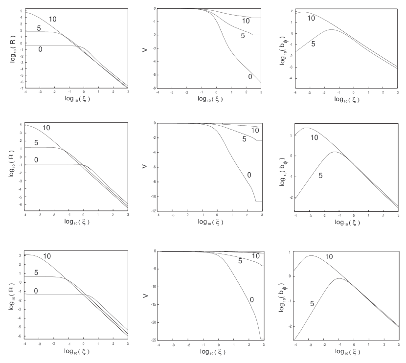
Figure 1: Profiles of the density, the radial velocity and the toroidal component of the magnetic field corresponding to $\gamma=0.9$ (top), $0.8$ (middle) and $0.7$ (bottom). Each curve is marked by the toroidal flux-to-mass ratio $\Gamma_{\rm\varphi}$.

We can find a family of limiting solutions for $\xi\rightarrow 0$. In order to obtain these, one can expand $R(\xi)$ and $V(\xi)$ in Taylor series

$$R(\xi)=R_{0}+R_{1}\xi+R_{2}\xi^{2}+\ldots$$ (24)

$$V(\xi)=V_{0}+V_{1}\xi+V_{2}\xi^{2}+\ldots$$ (25)

By substituting the above series in equations (11)-(14), we obtain the following limiting solutions for $\xi\rightarrow 0$ parameterized by $R_{0}$ and $\Gamma_{\rm\varphi}$:

$$R(\xi)=R_{0}-\frac{n(\pi+\Gamma_{\rm\varphi}^{2})}{n+1}R_{0}^{2-\frac{1}{n}}\xi^{2}+O(\xi^{4}),$$ (26)

$$V(\xi)=-\xi-\frac{\pi+\Gamma_{\rm\varphi}^{2}}{2(n+1)}R_{0}^{1-\frac{1}{n}}\xi^{3}+O(\xi^{5}),$$ (27)

$$b_{\rm\varphi}=\Gamma_{\rm\varphi}\xi[R_{0}-\frac{n(\pi+\Gamma_{\rm\varphi}^{2})}{n+1}R_{0}^{2-\frac{1}{n}}\xi^{2}+O(\xi^{4})].$$ (28)

Asymptotic solutions (26)-(28) are very useful when performing numerical integrations to obtain similarity solutions starting from $\xi\rightarrow 0$.

Table 1: Summary of the similarity solution for various $\gamma$ and $\Gamma_{\rm\varphi}$.

		$\gamma=0.9$				$\gamma=0.8$				$\gamma=0.7$
$\Gamma_{\rm\varphi}$	$\xi_{\ast}$	$R_{\ast}(\times 10^{2})$	$R_{\rm 0}$		$\xi_{\ast}$	$R_{\ast}(\times 10^{2})$	$R_{\rm 0}$		$\xi_{\ast}$	$R_{\ast}(\times 10^{2})$	$R_{\rm 0}$
0	2.99	$1.76$	0.37		3.20	2.57	0.12		3.54	2.29	0.04
1	2.87	$1.73$	0.56		3.09	2.54	0.17		3.22	2.62	0.07
2	2.67	$1.64$	1.45		2.66	2.58	0.45		2.57	3.17	0.25
3	2.51	$1.51$	4.73		2.44	2.40	1.52		2.48	2.82	0.54
4	2.40	$1.37$	16.8		2.31	2.16	4.89		2.32	2.56	1.49
5	2.35	$1.23$	63		2.24	1.90	16.32		2.23	2.27	4.36
6	2.32	$1.10$	246		2.22	1.66	56.2		2.20	1.98	12.85
7	2.33	$0.97$	980		2.23	1.44	200		2.21	1.70	39.30
8	2.34	$0.88$	3968		2.26	1.24	731		2.24	1.46	124
9	2.37	$0.78$	17866		2.31	1.07	2798		2.29	1.25	404
10	2.41	$0.69$	62700		2.36	0.93	10446		2.35	1.07	1386

3.3 numerical solutions

When similarity solutions cross the critical points, we must take extra care as for their analyticity across the critical points. In order to find the behaviour of solutions around critical point, $\xi=\xi_{\ast}$, we expand $R(\xi)$ and $V(\xi)$ in a Taylor series up to first order. Detailed calculations are in Appendix A. Given $\gamma$ and $\Gamma_{\rm\varphi}$, we can find analytical expressions for $\xi_{\ast}$ and $V_{\ast}$ as functions of $R_{\ast}$. However, note that only those points are acceptable that $\xi_{\ast}>0$ and $V_{\ast}<0$. Although we don’t study type of critical points in detail, when performing numerical integrations we note if the critical points are saddle or nodal (Jordan & Smith 1977). In general, the critical point is a saddle point when the two gradients of eigensolutions of $V(\xi)$ are of the opposite signs. On the other hand, when the two gradients have the same sign, the critical point is a nodal point.

We can numerically integrate equations (17) and (18) by a fourth order Runge-Kutta integrator. By using asymptotic solutions (26) and (27) for $\xi\rightarrow 0$, one can start integration of equations (17) and (18) at a very small $\xi$ ( e.g., $\xi=10^{-4}$) and with arbitrary value for $R_{0}$ for given $\Gamma_{\rm\varphi}$ and $\gamma$. Also, we can integrate the same equations (17) and (18) backward from the critical position, using asymptotic behaviour of solutions near the critical point for an arbitrary $R_{\ast}$. Thus, we look for matchings of $R$ and $V$ at some specific point $\xi_{\rm m}$ ($0<\xi_{\rm m}<\xi_{\ast}$). This can be found by studying loci in $V-R$ plane at $\xi_{\rm m}$.

Table 1 summarizes the dependence of the similarity solutions on $\Gamma_{\rm\varphi}$ and $\gamma$. Listed are the position of the critical point ($\xi_{\ast}$), the density at this point ($R_{\ast}$) and the density at the center ($R_{0}$). Figure 1 shows profiles of the density $R$, the radial velocity $V$ and the toroidal component of the magnetic field $b_{\rm\varphi}$ for different choice of $\gamma$ and $\Gamma_{\rm\varphi}$. Clearly the solutions except for the geometry and the magnetic field are equivalent to the Larson-Penston solution. In almost all cases, there are an inner part with approximately flat density profile and an outer region with decreasing density. Since the toroidal flux-to-mass ratio $\Gamma_{\rm\varphi}$ is constant during the collapse, each curve in Figure 1 is labeled by this ratio. For a fixed $\Gamma_{\rm\varphi}$, the central density increases as $\gamma$ increases. The infall velocity increases and tends to an asymptotic value at large radii. Of course, such large velocities are not acceptable and there must be a mechanism (e.g., pressure turncation) to turncate the solutions at finite radius. However, the typical behaviour of the radial velocity of a collapsing polytropic filament is different from the isothermal collapse where the self-similar infall velocity behaves in proportion to the radial distance. Also, Figure 1 shows that in the inner part the toroidal component of the magnetic field $b_{\rm\varphi}$ increases, while in the outer part $b_{\rm\varphi}$ is a decreasing function of $\xi$. This behaviour is easily understood, if we note $b_{\rm\varphi}=\Gamma_{\rm\varphi}\xi R$. For example, in the inner part, the density is roughly constant and so $b_{\rm\varphi}\propto\xi$.

An interesting feature of the solutions is that the cloud is more compressed by the toroidal pinching, if the toroidal magnetic field increases. Figure 1 shows that the size of the inner region strongly depends on $\Gamma_{\rm\varphi}$. However, the typical behaviours of the density and the magnetic field in the outer part are more or less independent of the toroidal field. We see that the central density increases, if $\Gamma_{\rm\varphi}$ increases so that in highly magnetized filament, the inner part with flat density profile disappears and joins to the outer region. If we compare the density profiles of $\gamma=0.9$ and $\gamma=0.7$ for $\Gamma_{\rm\varphi}=10$, we see there is still a small inner region for lower $\gamma=0.7$. It simply implies as $\gamma$ decreases, there needs higher level of magnetic intensity in order to affect the flat density profile of the inner part. In other words, as the cloud tends to the isothermal regime, the inner part becomes more sensitive on the toroidal magnetic field.

The infall velocity reduces as $\Gamma_{\rm\varphi}$ increases. While in nonmagnetic collapse, the radial velocity tends to very high value at large radii, we see that the velocity significantly reduces even at large radii in highly magnetized collapsing filament. However, the density profile in the outer region hardly depends on $\Gamma_{\rm\varphi}$. We find this profile mostly depends on $\gamma$, so that it behaves in proportion to $r^{-1.81}$, $r^{-1.69}$ and $r^{-1.55}$ at large radii for $\gamma=0.9$, $0.8$ and $0.7$, respectively. This typical behaviour of the density is in good agreement with the asymptotic solution at large radii which is expressed as $R(\xi)=R_{\infty}\xi^{-2/(2-\gamma)}$. Behaviour of the density profile at large radii does not change by increasing $\Gamma_{\rm\varphi}$ for a given $\gamma$. This behaviour is different from previous studies. Stodólkiewicz (1963) and Ostriker (1964) studied isothermal equilibrium structure of an isothermal filament, which the density falls off as $r^{-4}$ at large radii. Miyama et al. (1987) derived a set of self-similar solutions for an unmagnetized collapsing filament and their density structure is similar to unmagnetized equilibrium solutions, i.e. in proportion to $r^{-4}$ at large radii. TP showed that the density profile of an isothermal collapsing filament with purely toroidal magnetic field may change at large radii depending on the level of magnetization from $r^{-4}$ (low magnetization) to $r^{-2}$ (high magnetization). But we see as the cloud deviates from isothermality, these typical behaviours of the density profile at large radii change and the main parameter in shaping the profile is $\gamma$ not the level of magnetization, i.e. $\Gamma_{\rm\varphi}$.

Considering profile of the density in outer part of the filament, we can obtain the toroidal component of the magnetic field. Since at large radii we have $R\propto r^{\nu}$, the toroidal field becomes $b_{\rm\varphi}\propto r^{\nu+1}$, where $\nu=-1.81$, $-1.69$ and $-1.55$ for $\gamma=0.9$, $0.8$ and $0.7$, respectively. We discussed that the density profile at large radii is fairly insensitive to $\Gamma_{\rm\varphi}$, and it simply implies that the scaling of $b_{\rm\varphi}$ with the radial distance in the outer part is also insensitive to $\Gamma_{\rm\varphi}$. We can find behaviour of the ratio of the thermal to the magnetic pressures, $\beta$. One can easily show that in our notation the ratio is $\beta=(2/\Gamma_{\rm\varphi}^{2})(R^{\gamma-2}/\xi^{2})$. Thus, we see that in the inner part $\beta\propto r^{-2}$, irrespective of the value of $\gamma$ and $\Gamma_{\rm\varphi}$. But in the outer region we have $\beta\propto r^{(\gamma-2)\nu-2}$. These behaviours of $\beta$ show that during gravitational collapse of a polytropic, magnetized filament this ratio is not constant. However, the toroidal flux-to-mass ratio is conserved during collapse phase. In isothermal regime, one can assume either $\beta=constant$ or $\Gamma_{\rm\varphi}=constant$ and then study gravitational collapse (TP).

4 conclusion

In this paper, we have derived solutions able to describe dynamics of a collapsing, polytropic, magnetized, self-gravitating filament. The magnetic field is assumed to be purely toroidal, although it is the only possible magnetic configuration which can be studied using the similarity method (see below). But we expect our solutions to be a good approximation, if the poloidal fields are sufficiently weak. Moreover, purely toroidal field makes it easier to compare the obtained solutions with the isothermal collapse solutions as TP studied. Also, The self-similar solutions of our model can be used for future numerical or analytical studies because except for the geometry and magnetization they resemble to the Larson-Penston solution that has been found to be in good agreement with numerical analysis (e.g., Larson 1969; Hunter 1977; Foster & Chevalier 1993).

One may ask is it possible to extend this analysis by considering both the poloidal and the toroidal components of the magnetic field. We note that flux conservation imposes $B_{\rm z}\propto\rho$, which means the similarity solutions should support this scaling. However, such similarity solutions should be in these forms, according to a dimensional analysis: $B_{\rm z}=\mu^{\frac{1}{2}}K^{\frac{1}{2}}G^{-\frac{\gamma}{2}}(t_{0}-t)^{-\gamma}b_{\rm z}(\xi)$ and $\rho(r,t)=G^{-1}(t_{0}-t)^{-2}R(\xi)$. Obviously, this scaling does not support the flux conservation and so, it is necessary to put $b_{\rm z}=0$ or $B_{\rm z}=0$ . On the other hand, Hennebelle (2002) explored a set of self-similar solutions for a magnetized filamentary cloud, in which the toroidal and the poloidal components of the magnetic field play significant role in the dynamical collapse of the cloud. However, his solutions describe an isothermal, magnetized filamentary cloud which undergo collapse in the axial direction, in addition to radial collapse. In his model, the slope of the axial velocity being two times the slope of the radial one at the origin.

One of the major conclusions of our study is that the dynamics of a polytropic filament is different from the isothermal case. We showed that the toroidal component of the magnetic field help to confine the gas by hoop stress and this conclusion is independent of the exponent of the polytropic equation of state. Most measurements of molecular clouds have difficulty resolving the inner regions of filaments and so, it is very important to understand behaviour of the physical quantities at large radii. Our solutions showed that the typical behavior of the density of a magnetized polytropic filament mainly depends on polytrop index, $\gamma$, irrespective of the level of magnetization. However, the infall velocity in the outer regions strongly depends on the ratio of the flux-to-mass ratio $\Gamma_{\rm\varphi}$. It implies to examine the profiles of molecular lines for infall velocity which may help us to understand the true nature of the filaments. While radial velocity of the isothermal model of TP has a very simple behaviour, our polytropic solutions and Hennebelle (2002) model clearly present different profiles of the radial velocity similar to Larson-Penston solutions of collapsing unmagnetized spherical clouds.

The environment of L1512, a starless core, has been studied at high angular resolution by Falgarone, Pety & Philips (2001). The gas outside the dense core is structured in several filaments with a broad range of density and temperature, from $n_{\rm H_{\rm 2}}=2\times 10^{3}$ cm^-3 for the coldest case ($T=20$ K) down to $n_{\rm H_{\rm 2}}=180$ cm^-3 for the warmest ($T=250$ K). It suggests that a polytropic equation of state is more appropriate for describing the thermal behaviour of filaments of this system. Falgarone et al. (2001) discussed that these filaments are not held either by the pressure of the H _I layer or by the external pressure. So, they concluded that the toroidal component helps confine the filaments. However, their arguments were based on the analysis of Fiege & Pudritz (2000), in which the equilibria of pressure-truncated isothermal and logatropic filaments held by self-gravity and helical magnetic fields have been studied. However, it is unlikely that the filaments in ISM are being truly static structures, and many numerical simulations show dynamics structures in a star forming region (e.g., Vazquez-Semadeni et al. 2005; Jappsen et al. 2004). We think dynamics models, like what studied here, are more adequate for filamentary structures such as those in the environment of L1512 which show a wide range of density and temperature.

Acknowledgements: I thank the referee, Anthony Whitworth, for a careful reading of the manuscript and comments that lead to improvement of the paper.

Appendix A

To obtain accurate transonic solution, it is useful to analyze the behavior of the flow near the sonic point, $\xi_{\ast}>0$. The values of $R_{\ast}=R(\xi_{\ast})$ and $V_{\ast}=V(\xi_{\ast})$, where $V_{\ast}<0$, are completely determined by requiring both the denominator and numerator of equations (17) and (18) to vanish at $\xi_{\ast}$:

$$\gamma R_{\ast}^{\gamma-1}-U_{\ast}^{2}+\Gamma_{\rm\varphi}^{2}\xi_{\ast}^{2}R_{\ast}=0,$$ (29)

$$(2+\frac{V_{\ast}}{\xi_{\ast}})U_{\ast}+(1-\gamma)V_{\ast}-\frac{2\pi}{1-\gamma}R_{\ast}U_{\ast}-2\Gamma_{\rm\varphi}^{2}\xi_{\ast}R_{\ast}=0,$$ (30)

where $U_{\ast}=(2-\gamma)\xi_{\ast}+V_{\ast}$. In general, given $R_{\ast}$, it is a simple matter to find $\xi_{\ast}$ and $V_{\ast}$ from equations (29) and (30). After mathematical manipulation, we obtain

$$\xi_{\ast}=[\frac{-(ca+f)\pm\sqrt{(ca+f)^{2}+4h(cb-d)}}{2(cb-d)}]^{1/2}$$ (31)

where

$$a=\gamma R_{\ast}^{\gamma-1},b=\Gamma_{\rm\varphi}^{2}R_{\ast},c=(1-\frac{2\pi}{1-\gamma}R_{\ast})^{2},$$

$$d=[(1-\gamma)(2-\gamma)+\Gamma_{\rm\varphi}^{2}R_{\ast}]^{2},f=2ad^{1/2},h=a^{2}.$$

Now, we set

$$R(\xi)=R_{\ast}+a_{1}(\xi-\xi_{\ast})+O[(\xi-\xi_{\ast})^{2}],$$

$$V(\xi)=V_{\ast}+b_{1}(\xi-\xi_{\ast})+O[(\xi-\xi_{\ast})^{2}],$$

in neighborhood of $\xi_{\ast}$. Substitution of this first-order expansion in equations (17) and (18) leads to the following equations for the slopes $a_{1}$ and $b_{1}$:

$$a_{1}D_{1}-R_{\ast}X_{1}=0,$$ (32)

$$(2+b_{1}+\frac{V_{\ast}}{\xi_{\ast}})D_{1}+U_{\ast}X_{1}=0,$$ (33)

where

$$X_{\rm 1}=(\frac{b_{1}}{\xi_{\ast}}-\frac{V_{\ast}}{\xi_{\ast}^{2}})U_{\ast}+(2+\frac{V_{\ast}}{\xi_{\ast}})(2-\gamma+b_{1})+(1-\gamma)b_{1}-$$

$$\frac{2\pi}{1-\gamma}[a_{1}U_{\ast}+R_{\ast}(2-\gamma+b_{1})]-2\Gamma_{\rm\varphi}^{2}(R_{\ast}+a_{1}\xi_{\ast}),$$

$$D_{1}=\gamma(\gamma-1)R_{\ast}^{\gamma-2}a_{1}-2(2-\gamma+b_{1})U_{\ast}+$$

$$\Gamma_{\rm\varphi}^{2}\xi_{\ast}(a_{1}\xi_{\ast}+2R_{\ast}).$$

From equation (32), we have

$$a_{1}=-\frac{R_{\ast}}{U_{\ast}}(2+b_{1}+\frac{V_{\ast}}{\xi_{\ast}}),$$ (34)

and substituting in equation (33) gives an algebraic equation for $b_{1}$ as

$$Ab_{1}^{2}+Bb_{1}+C=0,$$ (35)

where

$$A=-\gamma(\gamma-1)\frac{R_{\ast}^{\gamma-1}}{U_{\ast}}-2U_{\ast}-\Gamma_{\rm\varphi}^{2}\frac{R_{\ast}\xi_{\ast}^{2}}{U_{\ast}},B=B_{1}+B_{2}+B_{3},C=U_{\ast}(C_{1}+C_{2})+(2+\frac{V_{\ast}}{\xi_{\ast}})C_{3},$$

$$B_{1}=U_{\ast}(3-\gamma+\frac{V_{\ast}}{\xi_{\ast}}+\frac{U_{\ast}}{\xi_{\ast}}+2\Gamma_{\rm\varphi}^{2}\frac{R_{\ast}\xi_{\ast}}{U_{\ast}}),B_{2}=(2+\frac{V_{\ast}}{\xi_{\ast}})[A-\gamma(\gamma-1)\frac{R_{\ast}^{\gamma-1}}{U_{\ast}}],B_{3}=2\Gamma_{\rm\varphi}^{2}R_{\ast}\xi_{\ast}-\Gamma_{\rm\varphi}^{2}(2+\frac{V_{\ast}}{\xi_{\ast}})\frac{R_{\ast}\xi_{\ast}^{2}}{U_{\ast}}-2(2-\gamma)U_{\ast},$$

$$C_{1}=(2+\frac{V_{\ast}}{\xi_{\ast}})(2-\gamma+\frac{2\pi R_{\ast}}{1-\gamma})-\frac{V_{\ast}U_{\ast}}{\xi_{\ast}^{2}},C_{2}=2\Gamma_{\rm\varphi}^{2}(2+\frac{V_{\ast}}{\xi_{\ast}})\frac{R_{\ast}\xi_{\ast}}{U_{\ast}}-2[\frac{\pi(2-\gamma)}{1-\gamma}+\Gamma_{\rm\varphi}^{2}]R_{\ast},C_{3}=B_{3}-\gamma(\gamma-1)(2+\frac{V_{\ast}}{\xi_{\ast}})\frac{R_{\ast}^{\gamma-1}}{U_{\ast}}.$$

References

- [] Bodenheimer, P., Sweigart, A., 1968, ApJ, 152, 515
- [] Bouquet, S., Feix, M. R., Fijalkow, E., Munier, A. 1985, ApJ, 293, 494
- [] Falgarone, E., Pety, J., Philips, T. G., 2001, ApJ, 555, 178
- [] Fiege, J. D., Pudritz, R. E., 2000, MNRAS, 311, 85
- [] Foster, P., Chevalier, R., 1993, ApJ, 416, 303
- [] Hennebelle, P., 2003, A&A, 397, 381
- [] Harjunpaa, P., Kaas, A. A., Carlqvist, P., Gahm, G. F. 1999, A&A, 349, 912
- [] Houlahan, P., Scalo, J. M. 1992, ApJ, 393, 172
- [] Hunter, C., 1977, ApJ, 218, 834
- [] Hunter, C., 1986, MNRAS, 223, 391
- [] Jappsen, A. K., Klessen, R. S., Larson, R. B., Li, Y., MacLow, M. M. 2004, A&A, in press (astro-ph/0410351)
- [] Jordan, D. W., Smith, P., 1977, Nonlinear Ordinary Differential Equations, Oxford Univ. Press, Oxford
- [] Inutsuka, S., Miyama, S. M. 1992, ApJ, 388, 392
- [] Kawachi, T., Hanawa, T., 1998, PASJ, 50, 577
- [] Larson, R. B., 1969, MNRAS, 145, 271
- [] Miyama, S. M., Narita, S., Hayashi, C. 1987, Prog. Theor. Phys., 78, 1051
- [] Ostriker, J. 1964, ApJ, 140, 1056
- [] Penston, M. V., 1969, MNRAS, 144, 425
- [] Scalo, J., Vazquez-Semadeni, E., Chappell, D., Passot, T. 1998, ApJ, 504, 835
- [] Schneider, S., Elmegreen, B. 1979, ApJS, 41, 87
- [] Shadmehri, M., Ghanbari, G., 2001, 278, 347
- [] Shu, F. H., 1977, ApJ, 214, 488
- [] Stodólkiewicz, J. S. 1963, Acta Astronomica, 13, 30
- [] Tilley, D. A., Pudritz, R. E., 2003, ApJ, 593, 426 (TP)
- [] Vázquez-Semadeni, E., Kim, J., Shadmehri, M., Ballesteros-Paredes, J., 2005, ApJ, in press
- [] Whitworth, A., Summers, D., 1985, MNRAS, 214, 1