ISO observations of 3 $-$ 200 $\mu$m emission by three dust populations in an isolated local translucent cloud

Abstract

We present ISOPHOT spectrophotometry of three positions within the isolated high latitude cirrus cloud G 300.2 $-$ 16.8, spanning from the near- to far-infrared. The positions exhibit contrasting emission spectrum contributions from the UIBs, very small grains and large classical grains, and both semi-empirical and numerical models are presented. At all three positions, the UIB spectrum shapes are found to be similar, and the large grain emission may be fitted by an equilibrium temperature of $\sim$17.5 K. The energy requirements of both the observed emission spectrum and optical scattered light are shown to be satisfied by the incident local ISRF. The FIR emissivity of dust in G 300.2 $-$ 16.8 is found to be lower than in globules or dense clouds, and is even lower than model predictions for dust in the diffuse ISM. The results suggest physical differences in the ISM mixtures between positions within the cloud, possibly arising from grain coagulation processes.

1 Introduction

1.1 UIBs and G 300.2 $-$ 16.8

A wide range of Galactic astrophysical objects exhibit infrared (IR) emission spectra clearly arising from multiple components in the solid- and gas-phases. Emission in the so-called Unidentified Infrared Bands (UIBs or UIR bands, also termed Infrared Emission Features, or IEFs) is significant in a wide range of sources. It often makes up as much as $20-30$ per cent of the total IR emission, and is thought to arise due to the presence of carbonaceous material of some kind. Although solid-phase carbonaceous grain components have been suggested, e.g. hydrogenated amorphous hydrocarbon (HAC; Jones, Duley & Williams 1990), quenched carbonaceous composites (QCC; Sakata & Wada 1989) or coal (Papoular et al., 1989), the bands are still widely attributed to gas-phase material. Typically, large free-floating aromatic species such as Polycyclic Aromatic Hydrocarbons (PAHs) are proposed (Léger & Puget 1984; Allamandola, Tielens & Barker 1985), and are usually thought to be ionized or to feature modified hydrogenation states. PAHs are excited by incident UV/visual radiation and subsequently re-emit in the IR at the specific UIB wavelengths. Observations have revealed that the bands are ubiquitous, appearing towards a range of regions such as Planetary Nebulae (PNe), HII regions and reflection nebulae around early-type stars. The presence of the 3.3- and 6.2-$\mu$m bands was mapped by AROME observations of the diffuse Galactic disc emission (Giard et al. 1996; Ristorcelli et al. 1994) and the full spectrum between 5 and 11.5 $\mu$m by ISOPHOT and IRTS spectrophotometry towards the inner Galaxy (Mattila et al. 1996; Tanaka et al. 1996; Onaka et al. 1996). Kahanpää et al. (2003) recently observed the inner Galaxy ($\mid l\mid\leq 60^{\circ}$, $\mid b\mid\leq 1^{\circ}$) UIB spectrum from $5-11.5$ $\mu$m along 49 sightlines using ISOPHOT data. IRTS results for several areas at $\mid b\mid\leq 4^{\circ}$ both in the inner and outer Galaxy have been presented by Sakon et al. (2004). The band strengths have also been mapped along the disc of an edge-on spiral galaxy (NGC 891) similar to the Milky Way (Mattila, Lehtinen & Lemke, 1999), and subsequently in other spiral galaxies (Lu et al., 2003).

The first discovery and measurement of the UIB emission in high latitude cirrus clouds was via their broadband IRAS 12-$\mu$m detections (Low et al. 1984; Boulanger, Baud & van Albada 1985; see Verter et al. 2000 and references therein). However, the first spectrally-resolved measurements of the bands toward an individual isolated cirrus cloud (G 300.2 $-$ 16.8) externally heated by the interstellar radiation field (ISRF) were made by Lemke et al. (1998, hereinafter L98) using the ISOPHOT instrument (Lemke et al., 1996) on board ESA’s ISO spacecraft (Kessler et al., 1996).

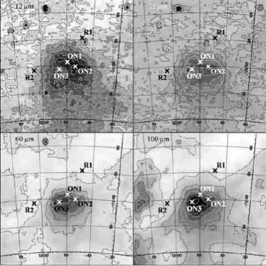
The cloud G 300.2 $-$ 16.8 is thought to be at the same distance of $150\pm 20$ pc from the Sun as the Chamaeleon clouds in general (Knude & Høg, 1998). Situated at $z\sim-40$ pc below the Galactic plane, it is well within the half-thickness of the local Galactic dust layer (see e.g. Neckel 1966). Bernard, Boulanger & Puget (1993) estimated G 300.2 $-$ 16.8 to have a diameter of $\sim$ 3 pc and a mass of 60 $M_{\sun}$. IRAS photometry indicated that the emission at 12, 25, 60 and 100 $\mu$m peaks at different positions within the cloud, suggesting that the object could be used to probe potential differences in the dust composition and the ISRF.

The L98 $3.3-16$ $\mu$m observations of G 300.2 $-$ 16.8 determined that the UIBs toward this object had absolute intensities $\sim$1/1000th of those typically seen toward bright planetary or reflection nebulae, but with relative band intensities not markedly different from these environments. This claim of a similarly-shaped UIB spectrum was confirmed by ISOCAM-CVF spectroscopy (Boulanger, 1998). In addition, they reported a non-zero continuum level at 10 and 16 $\mu$m, which they attributed to a population of very small grains (VSGs).

1.2 Three-component model

A three-component IR dust model has been proposed by e.g. Puget & Léger (1989). The first of these components is a mixture of large aromatic organic ions or molecules (e.g. compact PAHs) of $10-1000$ atoms (Bakes et al. 2001 & references therein), that is thought to give rise to the UIBs. The second is a population of transiently-heated VSGs (Sellgren, 1984) producing non-thermal emission in the mid- to far-IR. These are widely believed to be carbonaceous in nature, despite tight cosmic abundance constraints on carbon (Snow & Witt 1996; Kim & Martin 1996). The third population is of larger ($\sim 100-2000$ Å) ‘classical’ dust grains emitting in thermal equilibrium in the far-IR ($\lambda\geq 80\mu$m) at normal ISM temperatures of $\leq$ 20K. This population corresponds to the large grains used in popular models such as those of Mathis (1996) and Li & Greenberg (1997), and may have a fluffy and/or core-mantle structure.

1.3 Comparison of UIB and dust emission

To date, however, there have been no comprehensive comparisons of the near- to far- IR emission spectra of these UIB-rich environments over a wide range of UV/optical field strengths. The acquisition of a uniform dataset in order to thoroughly investigate ISM models of this kind is therefore needed. The IRAS dataset only features four broad photometric bands (centred at 12, 25, 60 and 100 $\mu$m) and is consequently of limited use in terms of spectral coverage. Data obtained using DIRBE suffers from excessively coarse spatial resolution (0.7^∘). Furthermore, any additional FIR data subsequently acquired (e.g. via airborne experiments) have generally been piecemeal in nature. This situation changed with the advent of ISO, which offered an unprecedented combination of IR wavelength coverage and detector sensitivities. We therefore begin here a series of papers that will address the situation by presenting a more complete spectrophotometric dataset obtained using ISOPHOT. This first paper focuses on the isolated cirrus/translucent cloud G 300.2 $-$ 16.8, and significantly augments the number of photometric bands used, and hence the wavelength coverage, of the L98 dataset.

Using ISOPHOT-P1, P2, C100 and C200 between 3.1 and 200 $\mu$m, we observed the cirrus/translucent cloud G 300.2 $-$ 16.8 in the Chamaeleon dark cloud complex. G 300.2 $-$ 16.8 has previously been found to exhibit a large IRAS $I_{12\mu\rm{m}}$ / $I_{100\mu\rm{m}}$ ratio of 0.14 (Laureijs et al., 1989). Furthermore, the signal in the IRAS 12-, 25-, 60- and 100-$\mu$m bands peaks at different positions in the cloud, suggesting variations in the local dust composition. Nevertheless, ISOPHOT data presented in L98 supported the detection of a UIB spectrum with a shape similar to that of a high ISRF environment. The comparatively high Galactic latitude ($b=-16.8$ degrees) minimizes the risk of confusion with unrelated structures along the sightline.

In this paper, we present an analysis of the three dust components and their variation within a single cloud. Section 2 details the observations and our data reduction methods and Sect. 3 summarizes the results. In Sect. 4, we use USNO-B1.0 and 2MASS archive data to derive the extinction properties of the sightlines. Section 5 describes our first attempts to model the emission across the broad ISOPHOT wavelength range, using both semi-empirical and physical numerical models. In Sect. 6, we consider the energy budget of the cloud, and we estimate FIR opacities and column densities in Sect. 7. Section 8 offers some conclusions and discusses some of the astrophysical implications of this work, and we conclude with a summary of the key points in Sect. 9.

Figure 1: Infrared observations of the isolated cirrus cloud G 300.2 $-$ 16.8. The images are the IRAS maps for the four IRAS filter bands. Crosses mark the position of observed by us using the ISOPHOT instrument aboard the ISO spacecraft, where R1 and R2 are the off-source reference positions and ON1, ON2 and ON3 are the on-source positions. The contours for the 12-$\mu$m filter range from 1.2 to 2.6 in steps of 0.2. The contours for the 25-$\mu$m filter range from $4.7-6.1$ in steps of 0.2. The contours for the 60-$\mu$m filter range from $1.0-7.0$ in steps of 1.0. The contours for the 100-$\mu$m filter range from $10.0-28.0$ in steps of 3.0. Units are MJy sr^-1. Co-ordinates are $\alpha,\delta(B1950.0)$.

2 Observations and reductions

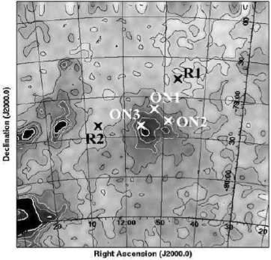
The observations were carried out during ISO revolutions 708 and 718 (1997 October 24 and 1997 November 3; for observation TDTs see Table 1). The observed on-source and reference positions match those in L98, with the three ON positions selected to coincide with the well-identified IRAS 12, 25 and 100-$\mu$m maxima (see Fig. 1).

Observations were performed in ten filters that are listed in Table 1, along with the PHT-P aperture diaphragm sizes or the PHT-C camera field sizes. The integration time was 32 seconds in all cases. The sparse map observing templates (AOTs 17/18/19: PHT-P and 37/38/39: PHT-C) were used (Klaas et al., 1994) and a separate sparse map was obtained using each filter. Since the sky brightness changes in the mid-IR bands by only a few percent between the different ON- and REF-positions in a given map, these modes were used to minimize detector drift effects that dominate the errors at these wavebands.

2.1 Reduction procedure

The data reduction was performed using the ISOPHOT Interactive Analysis Program (PIA) Version V9.0 (Gabriel, 2000). Essentially, the same reduction steps were applied as described in L98.

Landscape table to go here.

Table 1:

2.2 Calibration

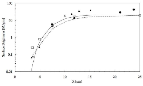
Our method utilizes the Zodiacal Light (ZL) as a calibration source. The basic technique was already used in L98 and has been described in more detail by Acosta-Pulido & Ábrahám (2001). The first and last measurements of each sparse map were paired with a measurement of the on-board calibration source FCS1 (Lemke et al., 1996), which was heated to give a signal corresponding to the expected sky brightness, yielding a first calibration. We then used the Zodiacal emission values from COBE/DIRBE to generate responsivity corrections for the resultant REF-position fluxes at wavelengths of $3-60\mu$m. The 60-$\mu$m cut-off point was chosen since the ZL no longer dominates the emission continuum longward of this wavelength. The photometric responsivity correction factors were determined by using the ISOPHOT ZL template spectrum ($5.9-11.7$ $\mu$m) of Leinert et al. (2002) most closely matching the G 300.2 $-$ 16.8 position (spectrum 8). The spectrum was rescaled to match the colour-corrected monochromatic COBE/DIRBE fluxes at 3.5, 5, 12 and 25 $\mu$m. This was fitted using a blackbody function, which was extrapolated out to 60 $\mu$m, and taken as the actual reference ZL levels. Figure 2 shows the Zodiacal emission spectrum out to 25 $\mu$m, the COBE/DIRBE measurements (Hauser, 1996), and our new photometry. The L98 data have been recalibrated using the improved ZL templates, again accounting for position and observation times. The derived scaling factors were applied to our colour-corrected (ON-REF) photometry.

2.3 Signal drift and foreground subtraction

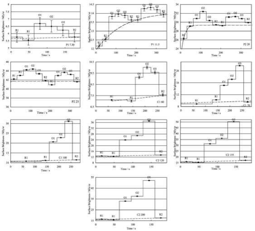
We display the observation sequences for the ten sparse maps in Fig. 3. In all ten of the filter bands, there is a clear excess signal in the ON positions. The detector drift has been modelled in one of two ways. For the cases where more than one measurement was made at each reference position, the background emission baseline was fitted using a function of the same form as that used in L98, otherwise a linear fit to the reference position data points was used. Subtraction of these fitted lines yielded the cloud emission. Photometric data were then corrected using standard ISO colour correction tables, to produce monochromatic fluxes directly comparable to those presented in L98. For filters with reference wavelengths greater than 20 $\mu$m, this was done by fitting either one or two modified blackbody functions of the form $\nu^{2}B_{\nu}$ and using the derived temperatures in conjunction with interpolated ISOPHOT colour correction lookup tables. No colour corrections were applied at the shorter wavelengths ($\lambda\leq 16\mu$m. For the C100 and C200 data, the surface brightness was determined from all of the detector array elements (3$\times$3 for C100 and 2$\times$2 for C200) in an attempt to optimally match the apertures used for the P1 and P2 measurements and hence minimize any possible systematic errors due to sampling area.

2.4 Error analysis

Statistical errors for the new data have been estimated by two methods, as in L98:

1. Internal errors, $\sigma_{\rm INT}$, for each measurement are obtained from the PIA analysis, and their means are given in column 9 of Table 1;

2. External errors, $\sigma_{\rm{EXT}}$, are obtained from the comparison of two independent measurements for O1, O2, O3 and R2 in the $10-25$-$\mu$m filters, and of three independent measurements of a reference position (R1 or R2) in the $7.3-7.7$-$\mu$m and $60-200$-$\mu$m filters.

For observation sequences which included two measurements of each ON position, the external errors were determined by using the differences of the three pairs of observations. After subtracting the ZL-background (modulated by detector drift effects), the two surface brightness measurements, $S_{A}$ and $S_{B}$, taken at each of the four positions POS$i$ (ON1, ON2, ON3 and the final pair of R2 measurements) were used to calculate the standard error of one measurement:

$$\sigma_{EXT}=\sqrt{\sum_{{\rm POS}i,i=1}^{4}(S_{A}-S_{B})^{2}/8}$$

These values were then reduced by a factor of $1/\sqrt{2}$ to obtain the standard error of the mean of the two measurements.

For the remaining bands, only one measurement was available for each ON position; external standard errors were therefore estimated in all but two of these cases from the scatter of the three measurements of the reference positions R1 and R2. These error estimates also include any detector drift effects and intrinsic differences between R1 and R2, and are therefore upper limits. Drift effects dominated the L98 7.3- and 7.7-$\mu$m band measurements, and so for these final two cases, external errors were instead estimated from the scatter of the three ON measurements. The resulting external error estimates, expressed in MJy sr^-1, are listed in column 10 of Table 1.

Systematic (calibration) errors

At wavelengths $3.3-25$-$\mu$m where the calibration was based on the Zodiacal Light (Sect. 2.2), the relative filter-to-filter errors depend on the accuracy of the shape of the zodiacal emission spectrum and the statistical accuracy of the G 300.2 $-$ 16.8 reference position measurements used in the calibrations (estimated to be $\sim$ 10 per cent). The absolute calibration accuracy also depends on the absolute zodiacal emission brightness in the COBE/DIRBE data. The adopted combined errors for the average ON minus REF cloud signal listed in the last column (14) of Table 1 were obtained by arithmetically adding the statistical external errors (column 11) and the filter-to-filter systematic (calibration) errors (column 12).

When estimating the filter-to-filter accuracies at $\lambda\geq 60\mu$m and the absolute accuracies at all wavelengths, the results of the Klaas et al. (2002) investigation of ISOPHOT accuracies were adopted. The estimated absolute accuracies are given in column 12 of Table 1. We note here that although the absolute accuracies for $\lambda\geq 60\mu$m are $\sim$ 20 $-$ 25 per cent, the filter-to-filter uncertainties for a single detector (e.g. C2) may be substantially smaller due to the elimination of most of the sources of error ( see del Burgo et al. 2003, Sect. 4). This issue is important in constraining the FIR temperature fits (see Sect. 5.1 and Table 3). Unlike the shorter-wavelength data, the absence of any independent calibration curve to aid cross-calibration for the $\lambda\geq 60\mu$m data dictated that the adopted combined errors for the average ON minus REF cloud signal listed in the last column (14) of Table 1 be obtained by arithmetically adding the statistical external errors (column 11) and the absolute errors (column 12).

Figure 2: Calibration of ISOPHOT photometry with COBE/DIRBE. The open squares represent the average of the COBE/DIRBE surface brightnesses at both REF positions for both observing dates. The filled circles represent the new photometry data after standard FCS1 calibration only. The solid curve represents the PHT-S and COBE/DIRBE-based averaged ZL spectrum adopted in this work. The dashed curve represents the ZL spectrum from L98. The small filled triangles represent the L98 photometry data after their standard FCS1 calibration only. The better agreement of the new data and the new ZL spectrum reflects improvements in both the normal FCS1 calibration and the techniques used in establishing the ZL spectrum.

Figure 3: Observed surface brightness in the different ISOPHOT filters prior to ZL recalibration and colour correction. The on-target and reference positions are designated as O1, O2, O3 and R1, R2 respectively. The measured values are plotted in the same sequence as they were measured. The dashed lines show fitted background zero levels. These were generally linear, except for the 11.5-, 20- and 25-$\mu$m filters, which used a fitted curve representing the detector drift. The surface brightness is given in the physical units (MJy/sr). The error bars shown indicate the internal statistical errors as obtained from the standard PIA reductions only. The time constants of the detector drift curves depend on the signal level, being smaller in the FIR detectors and when the signal is larger.

3 ISOPHOT results

The observed in-band power of the cirrus emission at the three ON positions is given in Table 2, combining the recalibrated data of L98 with the new data. Within errors, there is no disagreement between the pairs of P1_7.3 measurements, despite the difference in aperture sizes.

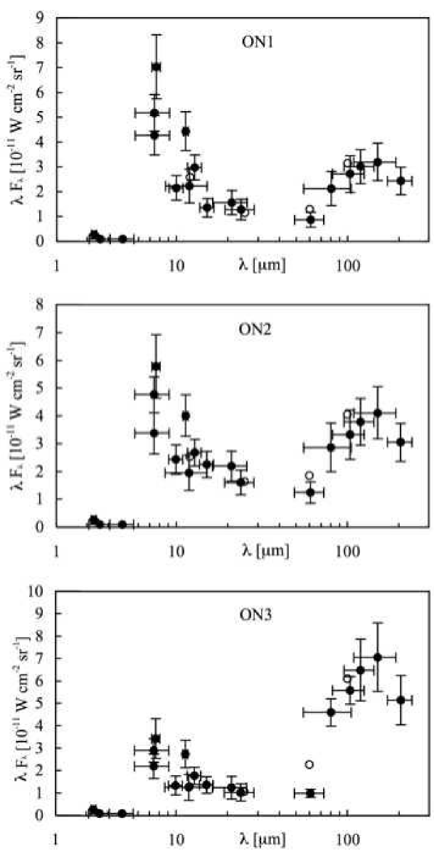
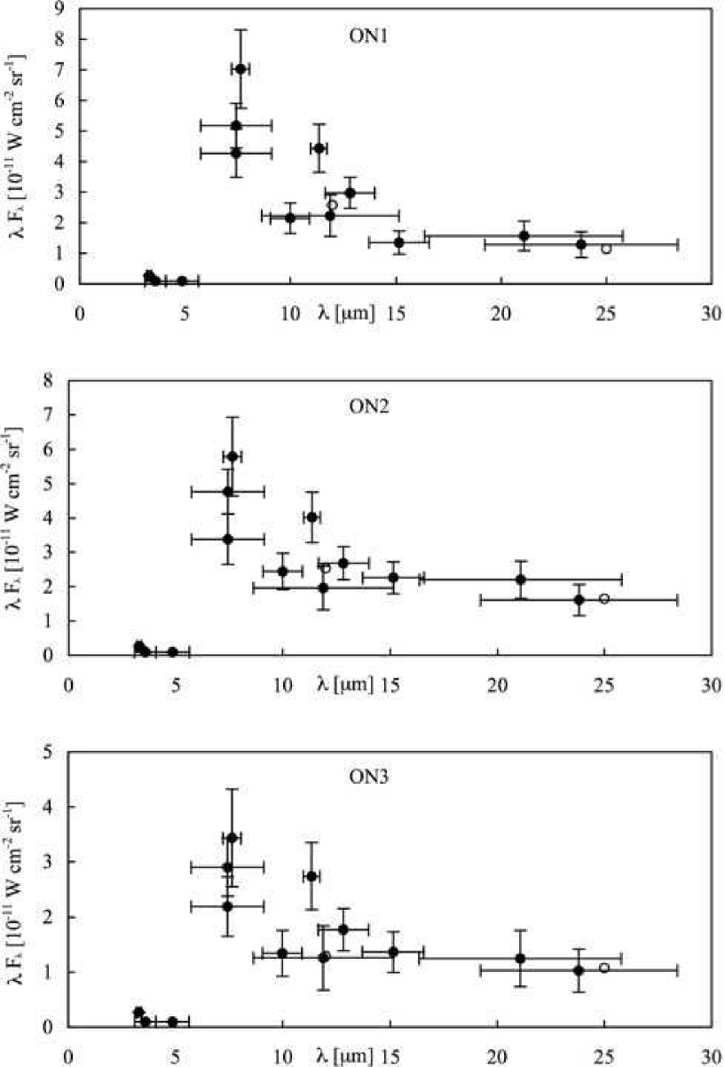
Figs. 4 and 5 show the photometric data for the three observed positions as spectral energy distributions. Qualitative differences in the relative strengths of the UIBs to the mid- and far-IR grain emission are immediately apparent. The spectrum at position ON1 clearly exhibits relatively strong UIBs, with the 7.7- and 11.3-$\mu$m bands demonstrating the importance of their carriers at this position. The UIBs are clearly the dominant factor that gives rise to a blue 12 $\mu$m/100 $\mu$m IRAS colour at ON1. At the ON2 position, the strongest of the UIBs (at 7.7 $\mu$m) and the thermal far-IR emission peak are at approximately the same level. Although still weaker than either of these, the mid-IR fluxes between 20 and 60 $\mu$m are at their relative maxima here, again in accordance with the high 25-$\mu$m IRAS value. The spectrum of position ON3 is dominated by the far-IR thermal emission from the larger dust grains, and the UIBs are comparatively weak. Another notable feature of the data is the clear presence of some form of underlying continuum emission, centred on a position longward of $\sim$10 $\mu$m.

Figure 4: Background-subtracted ISOPHOT photometry of the ON1, ON2 and ON3 positions (filled circles). The four IRAS fluxes are included for comparison (open circles). ISOPHOT data at $\lambda\geq 20\mu$m have been colour corrected. The horizontal bars reflect the effective filter band widths.

Figure 5: Background-subtracted ISOPHOT photometry of the UIB wavelength range at the ON1, ON2 and ON3 positions (filled circles). The two IRAS fluxes are included for comparison (open circles). ISOPHOT data at $\lambda\geq 20\mu$m have been colour corrected. The horizontal bars reflect the effective filter band widths.

Table 2: Positions, IRAS filter band ratios, extinctions and in-band emission powers of the cirrus cloud (bands+continuum) as observed with ISOPHOT in the different filter bands. Visual extinctions quoted here are based on the 2MASS mapping described in Sect. 4. The in-band powers are obtained here by multiplying the monochromatic fluxes by the filter widths, and are relative to a zero level determined at the reference positions (REF1: $\alpha=11^{\rm{h}}46^{\rm{m}}18.9^{\rm{s}},\delta=-78^{\circ}46^{\prime}33.2^{\prime\prime}$, REF2: $\alpha=12^{\rm{h}}06^{\rm{m}}23.4^{\rm{s}},\delta=-79^{\circ}22^{\prime}07.0^{\prime\prime};J2000.0$). The error estimates given in parentheses include (external) statistical errors and a relative filter-to-filter error or absolute accuracy (see column 14 of Table 1).

Position	ON1	ON2	ON3
$\alpha,\delta$ (J2000.0)	$11^{\rm{h}}52^{\rm{m}}08.3^{\rm{s}}$	$11^{\rm{h}}48^{\rm{m}}24.4^{\rm{s}}$	$11^{\rm{h}}55^{\rm{m}}33.8^{\rm{s}}$
	$-79^{\circ}09^{\prime}32.5^{\prime\prime}$	$-79^{\circ}17^{\prime}59.7^{\prime\prime}$	$-79^{\circ}20^{\prime}54.0^{\prime\prime}$
$A(V)$	$1.8\pm 0.2$	$1.9\pm 0.2$	$2.9\pm 0.2$
$A(V)$ (ON - REF)a	$1.2\pm 0.2$	$1.3\pm 0.2$	$2.3\pm 0.2$
$I_{\nu}(12)/I_{\nu}(100)$	0.11	0.08	0.029
$I_{\nu}(25)/I_{\nu}(100)$	0.094	0.105	0.044
$I_{\nu}(60)/I_{\nu}(100)$	0.244	0.273	0.223
$I_{\nu}(12)/I_{\nu}(25)$	1.17	0.762	0.659
Filter Band	In-band power, $P$ [$10^{-12}$ W cm-2 sr-1]
P(3.29)b	$\leq 0.18$	$\leq 0.18$	$\leq 0.18$
P(3.6)b	$\leq 0.27$	$\leq 0.27$	$\leq 0.27$
P(4.85)b	$\leq 0.31$	$\leq 0.31$	$\leq 0.31$
P(7.3)c	23.5(4.0)	21.7(4.1)	13.2(3.2)
P(7.3)d	19.4(3.0)	15.4(2.4)	10.0(1.9)
P(7.7)	7.7(1.4)	6.4(1.3)	3.8(1.0)
P(10)	4.0(0.9)	4.5(1.0)	2.5(0.8)
P(11.3)	3.0(0.5)	2.7(0.5)	1.9(0.4)
P(11.5)	12.2(3.7)	10.7(3.5)	6.9(3.2)
P(12.8)	5.4(0.9)	4.9(0.9)	3.2(0.7)
P(16)	2.6(0.7)	4.3(0.9)	2.6(0.7)
P(20)	7.0(2.2)	9.8(2.4)	5.6(2.3)
P(25)	4.9(1.6)	6.2(1.7)	4.0(1.5)
C(60)	3.4(1.2)	4.9(1.5)	3.9(0.7)
C(70)	13.1(4.2)	17.7(5.4)	28.4(3.8)
C(100)	11.4(3.1)	14.0(3.8)	23.6(2.6)
C(120)	12.0(2.7)	15.1(3.3)	25.8(5.5)
C(135)	17.6(4.1)	22.6(5.1)	38.9(8.4)
C(200)	8.0(1.8)	10.0(2.2)	16.9(3.6)

• $A(V)$ at reference position 1 = $0.7\pm 0.1$; $A(V)$ at reference position 2 = $0.5\pm 0.1$.

• Upper limits for bands+continuum, taken from table 3 of L98.

• L98; 180” aperture.

• This work; 99” aperture.

4 Optical extinction and scattered light

When describing the ISM in G 300.2 $-$ 16.8, knowledge of the $A(V)$ and $R(V)$ values are needed, where $R(V)\equiv A(V)/E(B-V)$. Star count data, i.e. the number of stars per square degree $N(m)$ brighter than magnitude $m$, in the $B_{J}$- and $I$-bands have been extracted from the USNO-B1.0 archive (Monet et al., 2003). We have used data from the second epoch SERC-$J$ ($B$-band) and SERC-$I$ ($I$-band) surveys. The value of the extinction $A$ is derived with the formula

$A=(1/k)$ log ($D_{ref}/D)$

where $k$ is the slope of the log $N(m)$ vs. $m$ relationship, $D_{ref}$ and $D$ are the stellar number densities at the reference area and at the cloud area. The values of $k$ and $D_{ref}$ have been determined from the reference area.

Figure 6: Extinctions obtained from star counts using the $B_{J}$ and $I$ band data of the USNO-B1.0 archive (Monet et al., 2003). The slopes for $R(V)$ = 3.05 and $R(V)$ = 5.0 are shown as dashed lines for comparison. The slope of the fitted line (continuous line) suggests $R(V)\sim 3.1$ for G 300.2 $-$ 16.8.

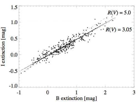
We have used $4700\AA$ and $8100\AA$ for the effective wavelengths of the $B_{J}$ and $I$ bands respectively (Gullixson et al., 1995). The observed relation between $B_{J}$ - and $I$-band extinctions is shown in Fig. 6. This yields the relation $A(I)=0.49\pm 0.01A(B_{J})$. Using the Cardelli, Clayton & Mathis (1989) extinction curve for the case of $R(V)=3.05$ this should be $A(I)=0.48A(B_{J})$ whereas for the $R(V)=5.0$ case, we would expect $A(I)=0.58A(B_{J})$.
The measured slope therefore suggests that $R(V)\sim 3.1$ for these sightlines, as would be expected for a diffuse cloud. It should be noted, however, that the photometric calibration of the USNO-B1.0 catalogue is still at a preliminary stage. This may give rise to an uncertainty in the $A(I)/A(B_{J})$ slope which could potentially dominate the inherent statistical errors as a consequence of calibration variations between survey plates. Consequently, only fields from one plate were included in the analysis.

The 2MASS $JHK_{S}$ data can be used to derive near-IR colour excesses of stars visible through G 300.2 $-$ 16.8, and hence derive NIR extinction. We have applied the optimized multi-band technique of Lombardi & Alves (2001). Stellar density for the stars which are detected at all three bands is constant throughout the map, with an average of 2.4 stars arcmin^-2.

The intrinsic colours of stars in the reference areas have the mean and standard deviations $(J-H)_{0}=0.45\pm 0.19$ and $(H-K_{S})_{0}=0.12\pm 0.21$. For the ratio of visual extinction to colour excess, we have used $A(V)/E(J-H)=9.90$ and $A(V)/E(H-K_{S})=14.70$, which correspond to $R(V)=3.05$.

Figure 7: $A(V)$ map obtained from the 2MASS $JHK_{S}$ colour excesses of stars visible through G 300.2 $-$ 16.8 via the multi-band colour excess method. The pixel size is 1.5 arcmin with a Gaussian FWHM = 4.0 arcmin used as a weighting function for the individual extinction values. The contours are from $A(V)$ = 0.5 to 3.5 mag in steps of 0.5 mag, with the contour or the local maximum near the centre of the field (near ON3 in G 300.2 $-$ 16.8) at the 3.0 level.

The pixel size of the extinction map was chosen to be 1.5 arcmin. The value of the extinction in each map pixel was derived from the individual extinction values of stars by applying the sigma-clipping smoothing technique of Lombardi & Alves (2001), and using a Gaussian with FWHM = 4.0 arcmin as a weighting function for the individual extinction values. There are two sources of variance in the extinction map; variance of the intrinsic colours $(J-H)_{0}$ and $(H-K)_{0}$, and variance of the observed magnitudes of the field stars. In the $A(V)$ map, the former source dominates with values of $\sim$0.15 magnitudes 1$\sigma$ error per pixel, while the latter source typically gives $\sim$0.05 magnitudes 1$\sigma$ error per pixel. The visual extinction map is shown in Fig. 7. This produced extinction values at the three ON positions of:

$A(V)$ (ON1) $=1.8\pm 0.2$

$A(V)$ (ON2) $=1.9\pm 0.2$

$A(V)$ (ON3) $=2.9\pm 0.2$

In order to constrain the energy budget of G 300.2 $-$ 16.8 (see Sect. 6 and 8.7), we have conducted optical $B_{J}$- and $R$-band surface photometry of the cloud. G 300.2 $-$ 16.8 appears on the same ESO/SERC sky survey plates as the Thumbprint Nebula (TPN). The $R$- and $B$-band photometry data presented in Lehtinen et al. (1998) and Fitzgerald, Stephens & Witt (1976) for the TPN were used to convert the photographic density values for G 300.2 $-$ 16.8 into $R$- and $B$-band surface brightnesses.

In addition, the $UBVRJHK$ surface photometry data for the TPN in Lehtinen et al. (1998) were taken as a template with which to estimate the $UBVRJHK$ SEDs for the G 300.2 $-$ 16.8 positions (see Fig. 10). The different optical depths, $\tau_{\lambda}$, for the TPN and G 300.2 $-$ 16.8 positions were taken into account by applying scaling factors of $(1-e^{-\tau_{\lambda}})$, and scaled to provide a best fit to the brightnesses at $B_{J}$ and $R$. The $\tau_{\lambda}$ values for G 300.2 $-$ 16.8 were determined from the measured $A(V)$ values using $R(V)=3.05$. From a comparison between the extinction-adjusted TPN template and the photometric values for G 300.2 $-$ 16.8, it can be concluded that:

1. The surface brightness SED template from the TPN reproduces the $B_{J}$ and $R$ measurements of G 300.2 $-$ 16.8 very well. It therefore appears reasonable to also use the TPN-based template as a first approximation for G 300.2 $-$ 16.8 shortward of the $B_{J}$- and longward of the $R$-band.
   

2. Using this purely empirical approach, we are not assuming that the dust scattering properties in G 300.2 $-$ 16.8 and the TPN are the same. There could also be a contribution by the Extended Red Emission (ERE) which, because of the consistency of the $B_{J}$- and $R$-band values, would have to be at similar relative levels in these two objects.
   

Consequently, the resultant values were assumed to broadly represent the optical surface brightness of G 300.2 $-$ 16.8.

5 Spectral modelling

5.1 Semi-empirical UIR band and FIR dust emission models

Based on the observed spectral energy distributions, modelling of the UIB emission is possible, if spectral feature profiles as observed in other Galactic emission regions are assumed. A number of types of line profile have previously been used by various authors attempting to describe the UIB spectrum, including Gaussian and Drude profiles (see table 7 of Li & Draine 2001b for a summary). Boulanger (1998) and Mattila, Lehtinen & Lemke (1999) found that astronomical spectra of the UIR bands could be well fitted to within ISOPHOT-S/ISOCAM-CVF resolutions using Cauchy/Lorentzian distribution functions. The advantage of the use of these profiles in model fits over Gaussians is that the need for an underlying plateau continuum emission between 5 and 9.5 $\mu$m is reduced, as the superposition of the wings of the Cauchy curves can account for more of the plateau emission. The curves may also be in accordance with the physical emission mechanisms of large molecules at high temperatures, with the Cauchy profiles being associated with the short excitation lifetime of vibrational states (Boulanger, 1998).

Our new data do not cover the 3.29- and 6.2-$\mu$m UIBs, and so the ISOPHOT photometry for these particular bands has not been improved upon since L98. On the other hand, an ISOCAM-CVF spectrum of a position coincident with the ON1 position has since been presented by Boulanger (1998). This spectrum may therefore be taken as indicative of the relative heights of the UIR bands, allowing reasonable assumptions to be made about the relative heights of some of the UIBs. A combination of this foreknowledge and our ISOPHOT photometry allows us to produce semi-empirical models of the UIR band emission spectra for our three positions in G 300.2 $-$ 16.8.

The 3.29-, 7.7-, 11.3- and 12.7-$\mu$m bands are covered by individual filters, which are sufficiently narrow as to enable a good characterization of the band heights. In contrast, the broad P7.3 filter spans a wavelength range encompassing the 6.2-, 7.7- and 8.6-$\mu$m bands, but still provides some constraints on emission. The model spectra are derived under the assumption of a Cauchy profile for each of the six expected major UIR bands. In addition to these, a continuum baseline function of the silicate dust emission spectrum from $2-18\mu$m, obtained from the physical modelling of the ON1 sightline (see Sect. 5.2 below), was also incorporated. The derived UIR band strengths are not strongly dependent on this specific choice of baseline function. Very similar results are obtained with other, more ad hoc baseline functions, e.g. a modified blackbody with $T\sim$300K, peaking near 10 $\mu$m, so the UIB modelling results are not dependent on an assumed enhancement of the small silicates population. Together, these functions produced a short wavelength model spectrum. This spectrum was then convolved with each of the ISOPHOT filter response curves in turn, and the resultant flux levels compared with the in-band power photometry values obtained with the P7.3, P7.7, P10, P11.3, P11.5, P12.8, P16 and P20 filters (Table 2). Parameters of the curves were then iteratively adjusted to minimize the $\chi^{2}$ statistic. Central wavelengths were determined first by fitting under the assumption of a spectrum similar to that of Boulanger (1998), and then fixed for subsequent detailed fitting. UIB widths for the 3.3-, 6.2-, 7.7-, 8.6- and 11.3-$\mu$m bands in the diffuse medium were taken from Kahanpää et al. (2003), and the width of the 12.7-$\mu$m band was allowed to vary between 0.27 and 1.18 $\mu$m, in accordance with the broad range of previously-reported function widths listed in Li & Draine (2001b). Due to the lack of narrow-band coverage of the 6.2-$\mu$m band by our dataset, an independent measurement of this band was not possible, and so height ratio constraints were applied, which were determined by comparing the Boulanger ISOCAM-CVF measurements taken near ON1 with average values obtained from Boulanger (1998) for Ophiucus and NGC 7023 and Mattila, Lehtinen & Lemke (1999) ISOPHOT-S observations of NGC 891. The two UIB height ratio constraints applied specified that 0.76 $\leq$ (6.2/7.7) $\leq$ 0.77 and 0.20 $\leq$ (8.6/7.7) $\leq$ 0.29.

The three longest-wavelength photometry points, C120, C135 and C200 are fitted using a modified blackbody function of the form $\nu^{2}B(\nu)$. This function is individually convolved with each of the three ISOPHOT filter response curves in turn, and the temperature and scaling are adjusted to best fit the photometry. In all three cases, a temperature of $\sim$17.5 K was obtained (Table 3). These temperatures reflect the average properties of the cloud, and do not preclude the possibility of colder grains near the cloud centre.

Figure 8: A modified blackbody fit of the form $\nu^{2}B_{\nu}(T)$ to the $120-200$ $\mu$m data points is shown as a black line spanning the $40-250$ $\mu$m wavelength range. Cauchy band profiles fitted to the $6.2-12.7$ $\mu$m UIBs are shown in red. A Li & Draine (2001b)-style silicate continuum is shown in blue for the $6.2-20$ $\mu$m range, and a combination of these is shown as a black line for $3-20$ $\mu$m.

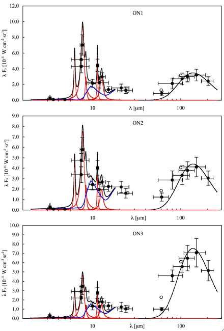
The resulting fits are shown in Fig. 8 and the parameters are listed in Table 3. It can be clearly seen from Fig. 8 that in all three cases, the middle range of the spectrum ($\sim$25 $-$ 70 $\mu$m) exhibits additional emission that cannot be accounted for by these two populations alone. Consequently, a third grain component in the infrared is required. As this arises due to non-equilibrium transient heating processes, detailed grain population modelling is required, as is described in Sect. 5.2. We also note that although the continuum near 10 $\mu$m does not appear to correlate strongly with the UIBs, Fig. 8 may indicate a correlation between the 10-$\mu$m continuum and the mid-IR emission from $\sim$16 $-$ 25 $\mu$m.

Table 3: Results of semi-empirical model fitting. Overall errors on the peak heights are estimated to be $\sim 20$ per cent, with relative band-to-band errors $\sim 10-15$ per cent. $F(\lambda)$ values are quoted in units of $10^{-12}$W cm${}^{-2}\mu\rm{m}^{-1}\rm{sr}^{-1}$.

Feature	Fit parameter	ON1	ON2	ON3
3.3-$\mu\rm{m}$	Central $\lambda$ $[\mu\rm{m}]$	3.29	3.29	3.29
banda	Width$[\mu\rm{m}]$	0.04	0.04	0.04
	$F(\lambda)$ Height	$\leq 1.47$	$\leq 1.47$	$\leq 1.47$
6.2-$\mu\rm{m}$	Central $\lambda$ $[\mu\rm{m}]$	6.27	6.27	6.27
band	Width$[\mu\rm{m}]$	0.24	0.24	0.24
	$F(\lambda)$ Height	9.5	7.6	4.7
7.7-$\mu\rm{m}$	Central $\lambda$ $[\mu\rm{m}]$	7.68	7.68	7.68
band	Width$[\mu\rm{m}]$	0.76	0.76	0.76
	$F(\lambda)$ Height	12.3	9.8	6.0
8.6-$\mu\rm{m}$	Central $\lambda$ $[\mu\rm{m}]$	8.40	8.40	8.40
band	Width$[\mu\rm{m}]$	0.33	0.33	0.33
	$F(\lambda)$ Height	3.5	2.8	1.7
11.3-$\mu\rm{m}$	Central $\lambda$ $[\mu\rm{m}]$	11.35	11.35	11.35
band	Width$[\mu\rm{m}]$	0.27	0.27	0.27
	$F(\lambda)$ Height	4.6	2.9	2.3
12.7-$\mu\rm{m}$	Central $\lambda$ $[\mu\rm{m}]$	12.64	12.64	12.64
band	Width$[\mu\rm{m}]$	1.18	1.18	1.18
	$F(\lambda)$ Height	2.4	1.6	1.2
7.7/11.3-$\mu\rm{m}$		$2.7\pm 0.4$	$3.4\pm 0.5$	$2.6\pm 0.4$
band ratio
10-$\mu\rm{m}$ continuum level		$2.3\pm 0.4$	$3.1\pm 0.6$	$1.8\pm 0.4$
(average of $F(\lambda)$ over $9.5-10.5$ $\mu\rm{m}$ range)
Classical grains: equilibrium		17.4	17.4	17.5
temperature, $T$ [K]		$\pm^{1.8}_{2.2}$	$\pm^{1.7}_{1.4}$	$\pm^{1.6}_{1.3}$

• Adopted from L98

5.2 Physical modelling

An alternative approach to the semi-empirical fit described in Sect. 5.1 is to construct a quantitative physical model of the cloud. Although a full numerical analysis is beyond the scope of this paper, we present here a first approximation of a three-component numerical model for G 300.2 $-$ 16.8. A detailed numerical model will be presented in a subsequent paper.

The numerical modelling code based on the Monte Carlo method (see Juvela & Padoan 2003 for full details) was applied. Spherical symmetry was assumed and clumping effects were neglected. The numerical model was applied to a grid of spherically-symmetric concentric shells. Due to the simple nature of the model, the library method of Juvela & Padoan (2003) was not used.

The Solar neighbourhood interstellar radiation field of (Mathis, Mezger & Panagia, 1983) as modified by Lehtinen et al. (1998) was adopted. The model clouds were discretized into 50 shells. The density was constant within the innermost 10 per cent of the cloud radius and in the outer parts the density decreased following power law $n\sim r^{-1.0}$. For each one of the three positions, ON1, ON2 and ON3, a separate cloud model was adopted, centred on each position in turn.

The dust properties were based on the Li & Draine (2001b) model. The dust consists of silicate grains (sizes $a>3.5$ Å), graphite grains ($a>50$Å) and PAHs (from $a=3.5\AA$ to $\sim 50\AA$) with optical properties corresponding to warm ionized medium. We have treated larger graphite grains ($a>50$ Å) and smaller graphite grains including the PAHs (from $a=3.5\AA$ to $\sim 50\AA$) as separate populations. As in Li & Draine, below 50 Å there is a smooth transition from the optical properties of graphite grains to PAH properties. The Li & Draine model was modified by removing emission features around 20 $\mu$m due to the lack of any such observed features in ISO SWS spectra. Between 15 $\mu$m and 36 $\mu$m, the absorption and scattering cross sections were replaced with values obtained with linear interpolation.

Monte Carlo methods were used to simulate the radiation field in the cloud. Temperature distributions of the grains were calculated in each cell based on the simulated intensity of the field (see Juvela & Padoan 2003). The dust emission spectrum, consisting of some 300 frequency points, was calculated towards the centre of the model cloud, and finally convolved with ISOPHOT filter profiles for direct comparison with observations.

The grain size distributions were modified in order to find the best correspondence between the model predictions and the observations. The size distributions of silicate grains and larger graphite grains were modified by a factor $\propto a^{\Delta\gamma}$, i.e. by changing the exponent of the size distribution by $\Delta\gamma$. The value of $\Delta\gamma$ was limited to a range [-1.5, +1.5]. PAHs and small graphite grains below 50Åwere treated as a separate population for which the shape of the size distribution was not modified. The total abundance of each of the three grain populations was treated as a free parameter.

Figure 9: Results of the physical modelling. The solid line shows the model spectra computed using the parameters listed in Table 4. The filled squares with the error bars are the observations and the open circles are the model predictions obtained by convolving the model spectrum with the corresponding filter profiles. The remaining curves show the components of the model spectrum: silicates (dashed line), large graphite grains (dash-dotted line) and small graphite grains including PAHs (dotted line).

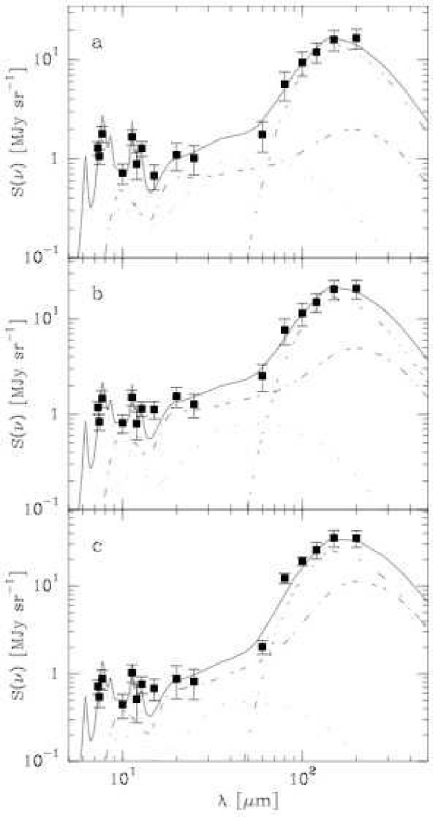
Figure 9 shows the fits, and Table 4 lists the obtained model parameters. The models preferred distributions with large graphite grains with $\Delta\gamma$ close to the allowed maximum value of 1.5 in all cases. The average size of the silicate grains was correspondingly decreased. The abundance of PAHs shows a strong variation, ranging from an overabundance by a factor of $\sim 3$ at the ‘halo’ position ON1 to an underabundance by a factor of $\sim 2$ at the centre position ON3. The derived visual extinction values giving the best fit agree with the $A(V)$ (ON - REF) values derived in Sect. 4 to within $\leq 26$ per cent.

Table 4: Parameters resulting from the physical modelling of the three source positions. The grain size distributions relative to the Li & Draine (2001b) model were modified by scaling the abundance by a factor $X$ and by changing the exponent of the size distribution, $\propto(a)^{\Delta\gamma}$. The allowed range for the values of $\Delta\gamma$ was [$-$1.5, 1.5]. For PAHs, only the abundance was changed. The abundances are given relative to the silicate component. The total dust column density resulting from the model fit is given as $A(V)$ ($R(V)=3.05$ has been used). The final row gives the total silicate abundance requirement, i.e. a factor by which the Li & Draine (2001b) model abundances have to multiplied.

		ON1	ON2	ON3
PAH	$X$	2.84	1.13	0.54
Graphite	$X$	0.57	0.31	0.73
	$\Delta\gamma$	1.47	1.48	1.50
Silicate	$X$	1.00	1.00	1.00
	$\Delta\gamma$	$-1.50$	$-1.38$	$-1.00$
$A(V)^{\mathrm{a}}$ [mag]		0.89	1.39	1.76
Silicate Abundance		1.50	3.25	2.09

• These values correspond to the $A(V)$ (ON - REF) values listed in Table 2.

In our modified Li & Draine-type model, the PAHs cannot explain the 10-$\mu$m continuum level as it stands. Excluding the unlikely possibility of another strong emission feature longward of 20 $\mu$m, either extra carbon absorption or small silicates must be invoked, in the following ways:

1. The 10-$\mu$m carbon absorption coefficient is increased, which effectively smoothes the continuum near 16 $\mu$m, or
   

2. The silicates are largely responsible for the 10-$\mu$m continuum level, while also producing a dip near 16 $\mu$m, which initially looks like a 22-$\mu$m emission feature in the photometry.

Inspection of the components of the plots in Li & Draine (2001b, e.g. their fig. 8) suggests that the silicates provide a peak at 10 $\mu$m, a continuum dip around 16 $\mu$m and a shoulder near 20 $\mu$m. We have adopted this latter approach, as also shown in Fig. 8. We discuss these alternatives in Sect. 8.3.

Figure 10: Spectral Energy Distributions for ON1, ON2 and ON3. The components contributing to the energy balance in the different wavelength ranges are indicated: $I_{\rm{scat}}$ is the scattered UV $-$ NIR light, $I_{\rm{UIB}}$ is the UIB emission, $I_{\rm{MIR}}$ is the VSG MIR contribution and $I_{\rm{emit}}$ is due to the big grains. The total interstellar radiation field (ISRF) in the Solar neighbourhood is also shown both before and after extinction effects (solid and dashed lines respectively). The data points marked on each of the $I_{\rm{scat}}$ lines represents the emission in the $B_{J}$ and $R$ bands, obtained by plate calibration with the TPN (see Sect. 4).

6 ISRF and the energy budget

The ISRF is the heating source of the dust grains in clouds lacking internal heating sources. The grains absorb photons in the ultraviolet to near-IR range, and subsequently emit photons at mid- to far-IR wavelengths corresponding to their temparature.

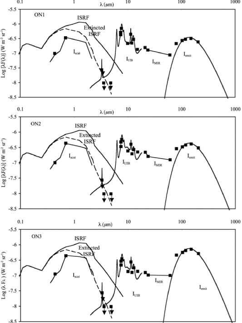
The energy emitted by the large grains, $I_{\rm{emit}}$, was obtained by integrating the modified blackbody fits from Sect. 5.1 over the wavelength interval 60 $-$ 1000 $\mu$m. We define $I_{\rm{UIB}}$ and $I_{\rm{MIR}}$ to be the areas under the empirical UIB curve and the observed 20 $-$ 60 $\mu$m filter fluxes, respectively. Given that the dust albedo is non- zero, some of the unabsorbed radiation is scattered from the cloud by the dust particles, producing optical and near-IR surface brightness. Taking the estimated optical SEDs obtained in Section 4, and integrating them over the wavelength range 0.36 $-$ 2.2 $\mu$m, we obtained the intensity of scattered radiation, $I_{\rm{scat}}$, for the three positions. The resultant energy budgets for the three sightlines, ON1, ON2, and ON3, are summarized in Table 5. The corresponding spectral energy distributions are shown in Fig. 10.

The solid ISRF lines in Fig. 10 represent the unattenuated local ISRF according to Mathis, Mezger & Panagia (1983) (hereafter MMP) as modified by Lehtinen et al. (1998): the intensities between 1.25 $-$ 2.2 $\mu$m were derived using the COBE/DIRBE all-sky data at the $J,H,$ and $K$ bands, and the resulting ISRF intensities at these bands were 20 $-$ 50 per cent higher than the MMP ones, resulting in an integrated ISRF(0.091 $-$ 8 $\mu$m) intensity of $20.4\times 10^{-7}$ W m^-2 sr^-1, some 15 per cent larger than the MMP value of $17.3\times 10^{-7}$ W m^-2 sr^-1.

However, not all of the total incident ISRF intensity is relevant to the energy balance of the cloud: only the extincted part of the ISRF contributes. Consequently, we have estimated the fraction of the ISRF that suffers extinction in the cloud by taking into account the wavelength and spatial dependence of the optical depth through the cloud. The average radial dependence of extinction was derived using the 2MASS extinction data displayed in Fig. 7. A cloud diameter ($\phi$) of 0.8^∘ centered on position ON3 was adopted. Effective extinction factors were then derived by calculating the term in square brackets in equation 5 of Lehtinen et al. (1998). The ISRF spectrum was then reduced in accordance with these extinction factors and the resulting extincted ISRF intensity, $I_{\rm{ISRF}}^{\rm{ext}}$, is shown as a dotted line in Fig. 10 and its total intensity, integrated over 0.091 $-$ 8 $\mu$m, at the bottom row of Table 5.

The quantity to be compared with the extincted ISRF intensity is not, however, the integrated surface brightness at any individual position of the cloud, but the mean surface brightness over the cloud face, $\overline{I(\lambda)}$, integrated over all wavelengths (for details, see equations 5 and 6 of Lehtinen et al. 1998). In order to account for this, we have approximated G 300.2 $-$ 16.8 as a spherical cloud of diameter 0.8^∘ (c.f. Fig. 1) and determined from the two ESO/SERC and four IRAS maps the mean surface brightness within this boundary. The background level, determined at our reference positions, has been subtracted. The ratios of the mean surface brightness to the surface brightness values at the three ON positions are given in Table 6. Using these ratios, i.e. ESO/SERC $B_{J}$ and $R$ for $I_{\rm{scat}}$, IRAS 12 $\mu$m for $I_{\rm{UIB}}$, IRAS 25 and 60 $\mu$m for $I_{\rm{MIR}}$, and IRAS 100 $\mu$m for $I_{\rm{emit}}$, we have derived the three estimates for the total mean radiation $\overline{I_{\rm{tot}}}$ (row 6) and the average of the three estimates in row (7). The IRAS maps are thus being used to obtain an estimate for the spatial distribution over the cloud face, while the ISOPHOT data are used to determine its spectral distribution. Within the error limits, $\overline{I_{\rm{tot}}}$ is seen to be in good agreement with the extincted ISRF $(0.091-8\mu\rm{m})$ intensity.

To ensure that this result did not strongly depend on the selected cloud boundary, we also repeated this procedure using cloud diameters of 0.7^∘ and 0.9^∘. For all three boundaries tested, the ratios $\overline{I_{\rm{tot}}}/I_{\rm{ISRF}}^{\rm{ext}}$ were obtained. They were 0.99$\pm$0.05, 0.89$\pm$0.05, and 0.88$\pm$0.05 for 0.7^∘, 0.8^∘, and 0.9^∘, respectively. This suggests that a 0.8^∘ boundary is a reasonable assumption and that $\overline{I_{\rm{tot}}}$ and $I_{\rm{ISRF}}^{\rm{ext}}$ are equal within the error limits. We will discuss the details of the energy budget in Sect. 8.6.

Table 5: Summary of the energy budget.

ISM component and	Surface Brightness [$10^{-7}$ W m-2 sr-1]
wavelength integration
range	ON1	ON2	ON3
Scattered radiation, $I_{\rm{scat}}$	$4.0\pm 1.0$	$5.0\pm 1.3$	$5.6\pm 1.4$
$(0.36-2.2\mu\rm{m})$
UIB emission, $I_{\rm{UIB}}$	$3.6\pm 0.7$	$3.6\pm 0.7$	$2.2\pm 0.4$
$(6-18\mu\rm{m})$
VSG MIR emission, $I_{\rm{MIR}}$	$1.4\pm 0.3$	$1.9\pm 0.4$	$1.2\pm 0.2$
$(21-60\mu\rm{m})$
Large grain emission, $I_{\rm{emit}}$	$3.6\pm 0.7$	$4.6\pm 0.9$	$7.9\pm 1.6$
$(60-1000\mu\rm{m})$
Total radiation, $I_{\rm{tot}}$	$12.7\pm 2.7$	$15.1\pm 3.3$	$16.9\pm 3.6$
(scattered + emitted)
Estimated $\overline{I_{\rm{tot}}}$	$10.4\pm 2.4$	$10.6\pm 2.5$	$11.5\pm 2.7$
for $\phi=0.8^{\circ}$ area
Average $\overline{I_{\rm{tot}}}$ for $\phi=0.8^{\circ}$ area		10.8 $\pm 2.5$
Total ISRF, $I_{\rm{ISRF}}(0.091-8\mu\rm{m})^{\mathrm{a}}$		20.4
Extincted ISRF, $I_{\rm{ISRF}}^{\rm{ext}}(0.091-8\mu\rm{m})$		12.2

• Mathis, Mezger & Panagia (1983) as modified by Lehtinen et al. (1998)

Table 6: Surface brightness ratios $\overline{I(\phi=0.8^{\circ})}$/$I$(ONi). The estimated errors are 10 per cent.

	ON1	ON2	ON3
Wavelength Band:
$B_{J}$	1.00	0.98	0.88
$R$	0.82	0.63	0.63
IRAS 12$\mu$m	0.65	0.66	1.29
IRAS 25$\mu$m	0.80	0.56	0.86
IRAS 60$\mu$m	0.83	0.58	0.47
IRAS 100$\mu$m	0.89	0.69	0.46

7 Far-infrared opacity

We derive the ratio between the FIR optical depth $\tau_{\rm{em}}(\lambda)$ and the optical extinction, $\tau_{200}/A(V)$ as well as the average absorption cross section per H-atom, $\sigma_{\lambda}^{\rm{H}}=\tau(\lambda)/N(H)$. If this ratio can be assumed to be the same from cloud to cloud, one can estimate the total cloud masses by using only the observed far-IR fluxes and the dust temperature derived from these fluxes (Hildebrand, 1983).

In the case of optically thin emission ($\tau$($\lambda$) $\ll$ 1) and an isothermal cloud, the observed surface brightness is

$I(\lambda)\approx\tau(\lambda)B(\lambda,T_{\rm{dust}})\propto\lambda^{-\alpha}B(\lambda,T_{\rm{dust}})$

We have derived the optical depths for $\alpha=2$ and for the $T_{\rm{dust}}$ values as given in Table 3. The resulting values of $\tau_{200}$ are listed in Table 7.

Table 7: Visual extinction, optical depth and average absorption cross-sections per H-nucleon for ON1, ON2 and ON3. $\tau_{200}$ is calculated under the assumption that $\tau_{\lambda}\propto\lambda^{-2}$.

	ON1	ON2	ON3
$A(V)$	$1.8\pm 0.2$	$1.9\pm 0.2$	$2.9\pm 0.2$
$N(H)$ $[10^{21}$ cm${}^{-2}]$ a	$3.5\pm 0.4$	$3.7\pm 0.4$	$5.66\pm 0.4$
$I_{200}(\nu)$ [MJy sr-1]	$16.6\pm 3.4$	$20.8\pm 4.3$	$35.2\pm 7.2$
$\tau_{200}$ $[10^{-4}]$	$1.9\pm 0.2$	$2.4\pm 0.2$	$4.0\pm^{0.4}_{0.3}$
$I_{200}/A(V)$ [MJy sr-1]	$9.2\pm 2.1$	$11.0\pm 2.5$	$12.1\pm 2.6$
$\tau_{200}/A(V)$ $[10^{-4}\rm{mag}^{-1}]$	$1.1\pm 0.2$	$1.3\pm 0.2$	$1.4\pm^{0.2}_{0.1}$
$\sigma_{200}^{\rm{H}}=\tau_{200}/N(H)$	$0.6\pm^{0.1}_{0.2}$	$0.7\pm 0.1$	$0.7\pm 0.1$
$[10^{-25}\rm{~{}cm}^{2}\rm{~{}H~{}nucleon}^{-1}]$

• The total hydrogen column density $N(H)$ is derived from $A(V)$ using the $N(H)$ vs. $E(B-V)$ relationship of Bohlin, Savage & Drake (1978) and $R(V)=3.05$.

Using the NIR extinction values derived in Sect. 4 or the equivalent $A(V)$ values as given in Table 2, we can derive values for $I_{200}/A(V)$ and $\tau_{200}/A(V)$, as given in Table 7.

We can also use the extinction for estimating the total hydrogen column densities, $N(H+H_{2})$. As a starting point, we adopt the value of $N(H+H_{2})/E(B-V)=5.8\times 10^{21}\rm{cm}^{-2}\rm{mag}^{-1}$ for diffuse clouds (Bohlin, Savage & Drake, 1978), together with $R(V)=3.05$ to obtain $N(H+H_{2})/A(V)=1.90\times 10^{21}\rm{cm}^{-2}\rm{mag}^{-1}$. We thus derive for G 300.2 $-$ 16.8 the total hydrogen column densities as shown in Table 7, and from these we calculate the values of $\sigma_{\lambda}^{\rm{H}}$, as listed in the last line of Table 7.

8 Discussion

8.1 ON1, ON2, ON3 in comparison with diffuse ISM sightlines

Our three observed ON positions in G 300.2 $-$ 16.8 cover a wide range of IRAS band ratios, $I_{12\mu\rm{m}}/I_{25\mu\rm{m}}$ and $I_{12\mu\rm{m}}/I_{100\mu\rm{m}}$, comparable to almost the whole range of these parameters as observed in a large sample of high-latitude diffuse and translucent clouds by Laureijs (1989). In this respect, the three SEDs for ON1, ON2 and ON3 may be considered as representative templates for diffuse/translucent sight lines in general. The three SEDs and their differences clearly suggest the presence of at least three MIR$-$FIR emitting dust components, with the UIBs strongest at ON1, the VSG emission making its largest relative contribution at ON2, and the large, classical grains dominating the IR emission spectrum at ON3.

The emission spectra derived from our data may be compared with those of previous datasets, such as the Dwek et al. (1997) SEDs produced using COBE data. The Dwek et al. data were successfully modelled by them using a three-component model. In their work, PAHs provided the $3.5-4.9$-$\mu$m emission in their models, the MIR-range emission was provided by VSGs, and at wavelengths above 140 $\mu$m, the emission was dominated by $T\approx 17-20$ K graphite and $15-18$ K silicate grains, in general agreement with our observations. Their model featured lower elemental abundance requirements than preceding work: they only required $\sim$20 per cent of the total carbon to be in PAHs and $\sim$60$-$70 per cent in graphite, but all of the silicon was locked in silicate grains. Their SED represented an average over a mixture of several high-latitude diffuse and translucent ISM clouds. Subsequent work by Verter et al. (2000) indicated notable cloud-to-cloud variations in the mid-IR emission of high- latitude translucent clouds, which they attributed to abundance and composition differences in the grains. The spatial resolution of our ISO data has permitted us to detect similar such variations within a single cloud.

Figure 11: Comparison of semi-empirical modelling with other Galactic UIB spectra. The thick solid lines are the semi-empirical model fits described in Sect. 5.1 to our ISOPHOT data (open circles). The horizontal bars reflect the effective ISOPHOT band widths, including that of the 11.5-$\mu$m band (beyond the plotted wavelength range), which extends down to $\sim$8.64 $\mu$m. The histogram lines are the average spectrum of the six strongest spectra from Kahanpää et al. (2003), multiplied by appropriate scaling factors. The dashed lines are the strongest spectrum of Onaka et al. (1996), again multiplied by appropriate scaling factors.

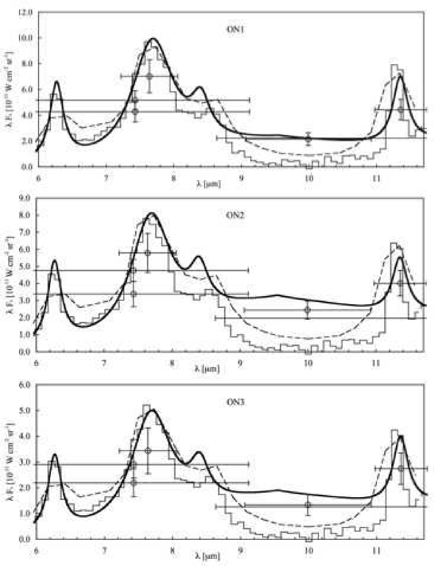
A comparison of the models with the shape of other Galactic UIB spectra from the literature further illustrates the similarities and differences of the sightlines. Fig. 11 compares the ON1, ON2 and ON3 with the observed average of the six strongest UIB spectra of Kahanpää et al. (2003) and the strongest spectrum of Onaka et al. (1996). Although the general shapes of the spectra are indeed similar, there are two notable differences in the $8-11$-$\mu$m range between our data and the other spectra. Firstly, the central position of the 8.6-$\mu$m UIB appears to be at a slightly shorter wavelength than previously observed. This arises due to our basing of the model on the Boulanger (1998) ISOCAM spectrum taken very close to ON1, which appears to show such properties. Furthermore, the lack of a narrow ISOPHOT filter band covering this feature means that the properties of the band in our model are not well constrained, hence, our model should only be taken as an approximation of this band’s wavelength. The second, more significant difference between our data and that of the Kahanpää et al. (2003) and Onaka et al. (1996) spectra is that the continuum near 10 $\mu$m is significantly higher in our spectra. This appears to be a genuine effect, and will be discussed in Sect. 8.3.

8.2 UIB properties

The UIB strengths have already been discussed in L98 and the present study confirms their results. Results obtained from the semi-empirical modelling of Sect. 5.1, listed in Table 3, suggest that the spectra can be fitted using a scalable continuum and a set of six Cauchy profiles, in good agreement with the CVF data of Boulanger (1998). Despite the differences in the continuum-subtracted band heights between positions ON1 and ON3, the ratio of the 7.7- and 11.3-$\mu$m UIB heights is similar, indicating that the relative carrier abundances are similar within errors. The 7.7 $\mu$m/11.3$\mu$m ratio at ON2 is rather higher than for the other two positions, but still within 30 per cent. Given the non-uniqueness of the underlying continuum used, together with the overall uncertainties on the photometry measurements, the spectrum does not appear significantly different. Furthermore, the UIB spectra appear to be similar to that seen in other interstellar environments (see e.g. table 7 of Li & Draine 2001b for a comparison).

8.3 Mid-IR continuum: PAHs vs. silicates

Our measured 10-$\mu$m continuum level in G 300.2 $-$ 16.8 has been confirmed by Boulanger (1998), and also reflects the continuum level in the Polaris cirrus cloud (Boulanger et al., 2000). The presence of an underlying continuum between the UIBs at 10 $\mu$m bears directly on the flux levels at 16 and 20 $\mu$m. On the basis of our observations, it appears that the 10-$\mu$m continuum level correlates more closely with the mid-IR emission at $16-25$ $\mu$m, rather than the UIBs (see Fig. 8 and Table 2). Under the assumption of a Li & Draine (2001b)-type model, there appear to be two alternative explanations for this continuum which does not appear in the Li & Draine (2001b) diffuse ISM results. The first is enhanced PAH emission through either a greater proportion of carriers, or enhanced particle emissivity. The second possibility is an excess of very small silicate particles.

In our physical modelling, the size distributions of silicate and graphite grains were modified by a factor $a^{\Delta\gamma}$, and the models preferred a large number of small silicate grains that accounted for much of the 10-$\mu$m continuum. There was a smooth change to PAH optical properties around $a\sim$50Å for graphite grains. Graphite grains above the 50Å limit do not provide any significant continuum at 10 $\mu$m. For the PAHs, both the optical properties and the shape of the size distribution were kept constant. Additional continuum at 10 $\mu$m could therefore only be provided in the models by small silicate grains. We might also consider the possibility that the increased continuum level could be produced equally well by small graphite grains ($\la$10Å). At positions ON2 and ON3, this would better account for the 16-$\mu$m observations that were underestimated in the numerical models (Fig. 9). However, (spherical) graphitic grains smaller than 10 Å would be difficult to incorporate on physical grounds. In the bulk form of graphite, the distance between graphene sheets is $\sim$ 3.35 Å, and the size of a unit cell carbon hexagon is $\sim$ 2.46 Å. These are both already a significant fraction of the proposed grain size, and for grains this small, some other assumptions (e.g. the heat capacities used or the assumption of a continuous energy spectrum) are also no longer strictly correct. Irrespective of the material forming these grains, however, the qualitative conclusion about the continuum level should still be valid.

Li & Draine (2001a) presented models with which they addressed the possible contribution to the diffuse ISM emission spectrum at $\lambda$ $\approx 10-30$ $\mu$m attributable to ultrasmall ($a<15$ Å) silicate dust grains. They also attempted to place upper limits on the presence of ultrasmall silicates via their contribution to the UV extinction curve. They estimated that as much as 10 per cent of the available interstellar silicon could be in ultrasmall silicates without violating any observational constraints.

In the physical models of Sect. 5.2, the relative amount of silicate was increased with respect to the amount of graphite. The final row of Table 4 summarizes the silicon abundance requirements of the models as a multiple of the Li & Draine (2001b) diffuse ISM requirement. The models all incorporate more silicate by a factor of $1.5-3.3$ than the Li & Draine (2001b) model. Furthermore, under the assumption of MgFeSiO₄ grains with a density 3.5 g cm^-3, the Li & Draine (2001b) models also have a silicon abundance requirement of $4.85\times 10^{-5}$, already higher than the Solar silicon abundance of $3.6\times 10^{-5}$. The amount of silicate needed could be reduced by changing the models, e.g. by employing a stronger radiation field. A separate population of small silicate (or graphite) grains might help to address the issue. Nevertheless, the availability of the amount of silicon needed will remain a problem.

Whatever the nature of the particles involved, there is now clear evidence of underlying emission that cannot be modelled using a first order polynomial, as has been done previously: there are differences between the baseline levels of the 6.2/7.7/8.6-$\mu$m and 11.3/12.7-$\mu$m groups. Even using a simple semi-empirical model, it is clear that this continuum appears to peak between 10 and 17 $\mu$m. Although a modelled silicate continuum has been used in the semi-empirical fitting in Sect. 5.1, we re-emphasize here that this is only an example of a possible fit, and does not necessarily suggest the presence of an excess of ultrasmall silicate grains.

8.4 The large ‘classical’ grains

Both the simple empirical fitting and the analytical Li & Draine (2001b)-type model are able to characterize the broader aspects of the big grain populations in G 300.2 $-$ 16.8. In all three sightlines, the grain emission in the long-wavelength ISOPHOT bands can be described by particles radiating at a stable temperature of $\sim$17.5 K (Table 3). These temperatures are in good agreement with Verter et al. (2000), who used DIRBE to survey and model eight translucent molecular clouds and reported temperatures of $\sim 16-18$K for the big grains. The study of high-latitude clouds by del Burgo et al. (2003) indicates a warm dust component with a temperature of $\sim$17.5 K. Earlier work by Dwek et al. (1997) also suggested that for wavelengths greater than 140 $\mu$m, their model was dominated by emission from T$\sim 17-20$K graphite and $15-18$K silicates. Li & Draine (2001b) also report temperatures of $13-22$K for a mixture of graphitic & silicate grains between 0.01 and 0.2$\mu$m. For the large grains, our numerical modelling adopted the properties described in Li & Draine (2001b). In our physical SED models, the graphite component dominates over the silicate component at wavelengths greater than $\sim$60 $\mu$m; thus we would expect our $\sigma_{\lambda}^{\rm{H}}$ values to be closer to that of graphite, which is also the case.

The listed $\sigma_{\lambda}^{\rm{H}}$ estimates for G 300.2 $-$ 16.8 were obtained using the methods of Hildebrand (1983). Li & Draine (2001b) have calculated absorption cross-sections for a diffuse dust model. The resulting $\sigma_{\lambda}^{\rm{H}}$ values are given in Table 8 for each of the grain components, i.e. graphite and silicate particles, as well as for the total mixture. For comparison with the observations, one must take into account that the observationally determined cross-section is a weighted sum of the graphite and silicate cross-sections, the weighting factor for the warmer graphite particles being larger than the one for the cooler silicates. This leads to the situation that in the Li & Draine (2001b) model, the contributions to the high-latitude emission spectrum by graphite and silicate grains are almost equal at $\lambda\sim 90-150$ $\mu$m (see their fig. 8). The effective cross-section as determined from the observed SED will thus be between the “graphite” and “silicate” values (see Mezger, Mathis & Panagia 1982 for details). It can be seen that the Li & Draine (2001b) calculated cross-sections are in reasonable agreement with our estimates for G 300.2 $-$ 16.8.

It appears, however, that the dust population composition towards G 300.2 $-$ 16.8 does not simply reflect the classic diffuse ISM picture. In Table 8, we also compare the ratios $\tau_{200}/A(V)$ and $\sigma_{\lambda}^{\rm{H}}=\tau_{200}/N(H)$ in G 300.2 $-$ 16.8 with a number of other interstellar clouds and dust models. While the Li & Draine (2001b) $\sigma_{\lambda}^{\rm{H}}$ values are generally consistent with our data, we note that the data in Table 8 suggest that our sightlines are different from the diffuse ISM. While it is unsurprising that the $\tau_{200}/A(V)$ and $\sigma_{\lambda}^{\rm{H}}$ values for the denser environments are much higher than for G 300.2 $-$ 16.8, we also note that the Dwek et al. (1997) diffuse ISM values are almost twice our G 300.2 $-$ 16.8 estimates. This suggests that the large grain population contribution is different for our sightlines, and that in general, smaller grains dominate in this region.

Table 8: Comparison of the 200-$\mu$m optical depth-to-$A(V)$ ratio and average absorption cross-section per H-atom nucleon for a range of ISM environments.

Object	$\tau_{200}/A(V)$	$\sigma_{200}^{\rm{H}}$	Reference
		$=\tau_{200}/N(H)$
	$[10^{-4}\rm{mag}^{-1}]$	$[10^{-25}$ cm2
		H nucleon${}^{-1}]$
G 300.2 $-$ 16.8
ON1	$1.1\pm 0.2$	$0.6\pm^{0.1}_{0.2}$	This work
ON2	$1.3\pm 0.2$	$0.7\pm 0.1$
ON3	$1.4\pm^{0.2}_{0.1}$	$0.7\pm 0.1$
Diffuse ISM	2.5	1.4	Dwek
			et al. (1997)
Thumbprint	5.3	$2.5_{-1.4}^{+3.2}$	Lehtinen
Nebula			et al. (1998)
(globule)
L183	$3.4-3.8$		Juvela et al.
(dense cloud)			(2002)
Model		2.7	Hildebrand
(molecular clouds)			et al.(1983)
Model		1.0 (silicates)	Li & Draine
(diffuse ISM)		0.53 (graphite)	(2001b)
		1.53 (total)

8.5 UIB/VSG/Large Grain emission variations

Extinction mapping and modelling of G 300.2 $-$ 16.8 by Laureijs et al. (1989) suggested that the variations of the relative emission strengths in the IRAS 12, 25, 60 and 100-$\mu$m bands between the centre and edge of the cloud cannot be solely attributed to ISRF attenuation effects, and they instead proposed that the variations are attributable to real abundance variations of the carrier populations. Modelling of the IR emission of G 300.2 $-$ 16.8 by Bernard, Boulanger & Puget (1993) also indicated that strong IRAS colour variations could not be attributed to radiative transfer effects alone. Their models instead suggested the presence of a halo of small dust particles and/or PAHs, with their densities decreasing towards the cloud interiors and giving way to the dominance of larger grains. This general picture is supported by our observations: ON3 is near the central part of the cloud, and ON1 and ON2 sample different halo positions.

More recently, surveys of MIR-FIR/submm dust emission have been conducted using data from the PRONAOS/SPM in conjunction with IRAS and COBE/DIRBE data for several sightlines (see Stepnik et al. 2003 for a review). Bernard et al. (1999) observed the high-latitude cirrus cloud MCLD 123.5 +24.9, which exhibited lower large grain equilibrium temperatures than other similar objects and a MIR emission deficit measured at 60 $\mu$m. The IRAS colours of this object already suggested an excess of cold dust, and the low temperature was attributed to a change in the dust properties and grain coagulation. Similar results for a molecular filament in the Taurus complex, coupled with the detection of corresponding submm enhancement, led Stepnik et al. (2003) to postulate that the effects there can be modelled by VSG-big grain coagulation into large fluffy aggregates.

Although G 300.2 $-$ 16.8 is at high Galactic latitude and does not show a 60-$\mu$m emission deficit in our data, we conclude that it is not a normal cirrus cloud. It has a relatively high average large grain temperature of $\sim$17.5 K for its estimated $A(V)$ at all three observed positions, and appears to exhibit a comparatively large number of small grains. The clear differences in the relative contributions to the emission spectrum by the UIBs, VSGs and large grains between the sightlines may be attributable to two scenarios:

1. Either the relative component population differences were established during the original cloud formation, and/or
   

2. Ongoing processing may give rise to material exchange between the populations (e.g. coagulation or fragmentation processes).

Distinguishing between these two possibilities may prove difficult, however, and might require statistical sampling of a number of clouds to conclusively determine whether anti-correlations exist between the components. Nevertheless, we note that for ON3, the increased large grain emission is accompanied by lowered UIB emission, which might suggest the accretion of the UIB carrier species on to large grains. Given that larger FIR emissivity appears to be needed for position ON3 (and possibly also for ON2) than for ON1, grain growth would seem plausible.

8.6 Energy budget and the ISRF

Within the error limits, the total surface brightness of G 300.2 $-$ 16.8, integrated from the UV to FIR wavelengths, was seen to be equal to the mean Solar neighbourhood ISRF intensity($0.091-8\mu\rm{m}$), extincted in the cloud (see Sect. 6 and Table 5). This supports the scenario in which G 300.2 $-$ 16.8 is solely heated by the external ISRF ($0.091-1.25\mu\rm{m}$). No associated stars are known of in G 300.2 $-$ 16.8 which could supply any noticeable additional heating radiation.

In the physical modelling of the SEDs in Sect. 5.2, the MMP ISRF as modified by Lehtinen et al. (1998) was adopted and a good agreement was found with the observed SEDs of positions ON1$-$ON3 not only with respect to their shape, but also with the absolute flux level. This indicates that the adopted ISRF intensity is of the correct magnitude to supply the heating power to the cloud. There are, however, other free parameters in the physical modelling, such as the line-of-sight dust column density (producing extinction) and the albedo of the grains, which can account for an error in the assumed ISRF intensity. The extinction by diffuse dust in the ‘envelope and intercloud region of the Chamaeleon dark cloud complex may be expected to attenuate the ISRF incident on G 300.2 $-$ 16.8 by $\sim$ 10 – 15 per cent. Taking this attenuation into account would increase the $A(V)$ estimates obtained from the physical modelling by $\sim$ 10 – 15 per cent, thus bringing them into better agreement with the directly observed $A(V)$ values.

The direct estimation of the energy balance, as presented in Sect. 6, does not depend on the detailed radiative transfer and dust modelling. Besides the adopted SED of the ambient ISRF, only observed quantities are involved, i.e. the extinction profile of the cloud and the UV-to-FIR surface brightness averaged over the cloud face. In this simple form, the approach is valid for clouds with spherical symmetry. This appears to be a reasonable assumption for G 300.2 $-$ 16.8 (see Figs. 1 and 7). The incident ISRF intensity is not isotropic, but shows a strong concentration towards the Galactic equator. For the cloud emission at mid- and far-infrared wavelengths, this causes no complications since the cloud emission is isotropic. However, at the UV-to-NIR wavelengths where the, predominantly forward-directed, scattering dominates, the surface brightness of the cloud depends on the viewing direction: a cloud of small-to-moderate optical depth is brighter when viewed in direction of the Galactic plane as compared to a viewing direction towards high Galactic latitudes. In the case of G 300.2 $-$ 16.8, the viewing direction is towards an intermediate Galactic latitude, $b=-16.8^{\circ}$, which means that the effective ISRF intensity for scattering is close to the average ISRF intensity over the sky (see Lehtinen & Mattila 1996 for details).

An interstellar cloud for which both the extinction profile and the UV-to-FIR surface brightness are measured can be used as a probe of its ambient ISRF intensity. This way, one could probe the ISRF within $\sim$ 1 kpc of the Sun in different environments, such as stellar associations or clusters with enhanced ISRF. The location of G 300.2 $-$ 16.8 in the Chamaeleon Cloud Complex is not expected to imply any significant enhancement of the ISRF: the young stars in Cha I and II clouds are mostly of low luminosity and many of them are still embedded in their parental cloud. The analysis of the energy balance of the Thumbprint Nebula, a globule also located in the Chamaeleon Complex, gave the same result, i.e. that its ambient radiation field can be well represented with the average Solar neighbourhood ISRF (see Lehtinen et al. 1998).

9 Summary

1. We have presented multi-wavelength ISOPHOT photometry of three differing sightlines corresponding to IRAS 12-, 25- and 100-$\mu$m photometry peaks within the G 300.2 $-$ 16.8 high latitude translucent cloud. The data cover the NIR$-$FIR wavelength range, and demonstrate the need for at least three ISM components: UIB carriers, transiently-heated VSGs and large classical grains at thermal equilibrium.
   

2. 2MASS $JHK_{S}$ colour excesses of stars visible through the cloud were used to construct an extinction map. Star counts in the $B_{J}$ and $I$ bands indicated a reddening law compatible with the diffuse dust $R(V)$ value.
   

3. The UIB section covered by filter photometry was fitted semi-empirically using a typical model silicate continuum and six Cauchy curves. An underlying continuum peaking around $15-16$ $\mu$m was found to be necessary. The emission by large grains was well fitted for all three sightlines with a modified blackbody curve of $T\sim$17.5 K. This is warmer than expected, but not incompatible with other observations of diffuse and translucent clouds. Emission was detected in the MIR range, which was attributed to non-thermal emission by transiently-heated small grains.
   

4. Under the assumption of simple spherical geometry, numerical modelling of the data, based on the work of Li & Draine (2001b), was performed. The models were able to fit the spectra plausibly. The differences in the SEDs cannot be explained by radiation field variations or radiative transfer effects. Abundance variations are required to explain the differences between (e.g.) the UIB carrier contributions to the cloud centre (ON3) and halo (ON1) spectra. Some very small silicate grains appear to be required by the models, with a greater quantity of silicon (and carbon) than is allowed by some current cosmic abundance estimates, but this is true of other existing models as well (e.g. Li & Draine 2001b).
   

5. The FIR opacity per nucleon, measured by the quantity $\sigma_{\lambda}^{\rm{H}}=\tau_{200}/N(H)$ , assumes values in G 300.2 $-$ 16.8 which are lower than some of the recently obtained values for globules and dense molecular clouds. The estimated values of $\tau_{200}/A(V)$ are also smaller than those obtained from recent diffuse ISM models, suggesting an enhancement of the small grain population.
   

6. Within errors, the energy of the sum of the optical scattered light and emission from the UIBs, VSGs and large grains can be supplied by the local ISRF. The relative amounts of the UIB, VSG and large grain emission vary as expected from the original IRAS photometry: UIB emission is strongest in ON1, the mid-IR VSG emission peaks at ON2, and the large grain emission dominates at ON3. It is not yet clear whether material is transferred between the three populations, and statistical sampling of a range of clouds may be required to address this issue in the future. The variations between the three sightlines appear to be a result of abundance variations of the three (or more) carrier populations within the cloud, and this may be due to grain coagulation processes.

References

- Acosta-Pulido & Ábrahám (2001) Acosta-Pulido J. A., Ábrahám P., 2001, in Metcalfe L., Kessler M. F. K., eds, The calibration legacy of the ISO Mission, ESA Special Publication Series, SP-481, p. 15
- Allamandola, Tielens & Barker (1985) Allamandola L. J., Tielens A. G. G. M., Barker J. R., 1985, ApJ, 290, L25
- Arendt, Dwek & Moseley (1999) Arendt R. G., Dwek E., Moseley S. H., 1999, ApJ, 521, 234
- Bakes et al. (2001) Bakes E. L. O., Tielens A. G. G. M., Bauschlicher C. W., Jr., Hudgins, D. M., Allamandola, L. J., 2001, ApJ, 560, 261
- Bernard, Boulanger & Puget (1993) Bernard J. -P., Boulanger F., Puget J. L., 1993, A&A, 277, 609
- Bernard et al. (1999) Bernard J. -P. et al., 1999, A&A, 347, 640
- Bohlin, Savage & Drake (1978) Bohlin R. C., Savage B. D., Drake J. F., 1978, ApJ, 224, 132
- Boulanger (1998) Boulanger F., 1998, in L. d’Hendecourt, C. Joblin, A. Jones, eds, Les Houches Workshop Conf. Proc. 11, Solid Interstellar Matter: The ISO Revolution, Springer, p. 19
- Boulanger, Baud & van Albada (1985) Boulanger F., Baud B., van Albada G. D., 1985, A&A, 144, L9
- Boulanger et al. (2000) Boulanger F., Abergel D., Cesarsky D., Bernard J. -P., Miville Deschênes M. A., Verstraete L., Reach W. T., 2000, in Laureijs R. J., Leech K., Kessler M. F., eds, ISO Beyond Point Sources, ESA Special Publication Series, SP-455, p. 91
- Cardelli, Clayton & Mathis (1989) Cardelli J. A., Clayton G. C., Mathis J. S., 1989, ApJ, 345, 245
- Chan & Onaka (2000) Chan K.-W., Onaka T., 2000, ApJ, 533, L33
- del Burgo et al. (2003) del Burgo C., Lauerijs R. J., Ábrahám P., Kiss, Cs., 2003, MNRAS, 346, 403
- Draine (1978) Draine B. T., 1978, ApJS, 36, 595
- Dwek et al. (1997) Dwek E. et al., 1997, ApJ, 475, 565
- Fitzgerald, Stephens & Witt (1976) Fitzgerald M. P., Stephens T. C., Witt A. N., 1976, ApJ, 208, 709
-
Gabriel (2000)
Gabriel C., 2000, PHT Interactive Analysis User Manual (V9.0)
www.iso.vilspa.esa.es/manuals/PHT/pia/um/pia_um.html - Giard et al. (1996) Giard M., Serra G., Caux E., Pajot F., Lamarre J. M., 1988, A&A, 201, L1
- Gullixson et al. (1995) Gullixson C. A., Boeshaar P. C., Tyson J. A., Seitzer P., 1995, ApJS, 99, 281
- Hauser (1996) Hauser M.G., 1996, in AIP Conf. Proc. Vol. 348, Dwek E., ed, Unveiling the Cosmic Infrared Background, p. 11
- Hildebrand (1983) Hildebrand R. H., 1983, QJRAS, 24, 267
- Jones, Duley & Williams (1990) Jones A. P., Duley W. W., Williams D. A., 1990, QJRAS, 31, 567
- Juvela & Padoan (2003) Juvela M., Padoan P., 2003, A&A, 397, 201
- Juvela et al. (2002) Juvela M., Mattila K., Lehtinen K., Lemke D., Laureijs R., Prusti, T., 2002, A&A 382, 583
- Kahanpää et al. (2003) Kahanpää J., Mattila K., Lehtinen K., Leinert C., Lemke D., 2003, A&A, 405, 999
- Keene et al. (1980) Keene J., Hildebrand R. H., Whitcomb S. E., Harper D. A., 1980, ApJ, 240, L43
- Kessler et al. (1996) Kessler M. F. et al., 1996, A&A, 315, L27
- Kim & Martin (1996) Kim S.-H., Martin P. G., 1996, ApJ, 462, 296
- Klaas et al. (1994) Klaas U., Krüger H., Heinrichsen I., Heske A., Laureijs, R., eds, 1994, ISOPHOT Observers Manual, version 3.1.1
- Klaas et al. (2002) Klaas U. et al., 2002, ISOPHOT Calibration Accuracies, Version 5.0, SAI/1998-092/Dc
- Knude & Høg (1998) Knude J., Høg E., 1998, A&A, 338, 897
- Kwok, Volk & Hrivnak (1989) Kwok S., Volk K. M., Hrivnak B. J., 1989, ApJ, 345, L51
- Kwok, Volk & Hrivnak (2002) Kwok S., Volk K., Hrivnak B. J., 2002, ApJ, 573, 720
- Laureijs (1989) Laureijs R.J., 1989, Ph.D. Thesis, Univ. Gronigen
- Laureijs et al. (1989) Laureijs R.J., Chlewicki G., Clark F.O., Wesselius P.R., 1989, A&A, 220, 226
- Léger & Puget (1984) Léger A., Puget J. L., 1984, A&A, 137, L5
- Lehtinen & Mattila (1996) Lehtinen K., Mattila K., 1996, A&A, 309, 570
- Lehtinen et al. (1998) Lehtinen K., Lemke D., Mattila K., Haikala L.K., 1998, A&A, 333, 702
- Leinert et al. (2002) Leinert C., Ábrahám P., Acosta-Pulido J., Lemke D., Siebenmorgen R., 2002, A&A, 393, 1073
- Lemke et al. (1996) Lemke D. et al., 1996, A&A 315, L64
- Lemke et al. (1998) Lemke D., Mattila K., Lehtinen K., Laureijs R. J., Liljestrom T., Léger A., Herbstmeier U., (L98) 1998, A&A, 331, 742
- Li & Draine (2001a) Li A., Draine B. T., 2001a, ApJ, 550, L213
- Li & Draine (2001b) Li A., Draine, B. T., 2001b, ApJ, 554, 778
- Li & Greenberg (1997) Li A., Greenberg J. M., 1997, A&A, 323, 566
- Lombardi & Alves (2001) Lombardi M., Alves J., 2001, A&A, 377, 1023
- Low et al. (1984) Low, F.J. et al., 1984, ApJ 278, L19
- Lu et al. (2003) Lu N. et al., 2003, ApJ 588, 199
- Mathis (1996) Mathis J. S., 1996, ApJ, 472, 643
- Mathis, Mezger & Panagia (1983) Mathis J. S., Mezger P. G., Panagia N., 1983, A&A, 128, 212
- Mattila et al. (1996) Mattila K., Lemke D., Haikala L. K., Laureijs R. J., Léger A., Lehtinen K., Leinert C., Mezger P. G., 1996, A&A, 315, L353
- Mattila, Lehtinen & Lemke (1999) Mattila K., Lehtinen K., Lemke D., 1999, A&A, 342, 643
- Mezger, Mathis & Panagia (1982) Mezger P. G., Mathis J. S., Panagia N., 1982, A&A, 105, 372
- Monet et al. (2003) Monet D. G. et al., 2003, AJ, 125, 984
- Müller (2000) Müller T. G., 2000, in Laureijs R. J., Leech K., Kessler M. F., eds, ISO Beyond Point Sources, ESA Special Publication Series, SP-455, p. 33
- Neckel (1966) Neckel T., 1966, Z. für Astrophys., 63, 221
- Onaka et al. (1996) Onaka T., Yamamura I., Tanabe T., Roellig T. L., Yuen L., 1996, PASJ, 48, L59
- Papoular et al. (1989) Papoular R., Conrad J., Giuliano M., Kister J., Mille G., 1989, A&A, 217, 204
- Parravano, Hollenbach & McKee (2003) Parravano A., Hollenbach D. J., McKee C. F., 2003, ApJ 584, 797
- Puget & Léger (1989) Puget J. L., Léger A., 1989, ARA&A, 27, 161
- Ristorcelli et al. (1994) Ristorcelli I., Giard M., Meny C., Serra G., Lamarre J. M., Le Naour C., Leotin J., Pajot F., 1994, A&A, 286, L23
- Sakata & Wada (1989) Sakata A., Wada S., 1989, in Allamandola L. J., Tielens A. G. G. M., eds, Proc. IAU Symp. 135, Interstellar dust, Santa Clara, Dordrecht, p 191
- Sakon et al. (2004) Sakon I., Onaka T., Ishihara D., Ootsubo T., Yamamura I., Tanabé T., Roellig T. L., 2004, ApJ, 609, 203
- Sellgren (1984) Sellgren K., 1984, ApJ, 277, 623
- Snow & Witt (1996) Snow T. P., Witt A. N., 1996, ApJ, 468, L65
- Stepnik et al. (2003) Stepnik B. et al., 2003, A&A, 398, 551
- Tanaka et al. (1996) Tanaka M., Matsumota T., Murakami H., Kawada, M., Noda M., Matsuura S., 1996, PASJ 48, L53
- Verter et al. (2000) Verter F., Magnani L., Dwek E., Rickard L. J., 2000, ApJ, 536, 831
- Volk, Kwok & Hrivnak (1999) Volk K., Kwok S., Hrivnak B. J., 1999, ApJ, 516, L99