Pushing the Boundaries of the Cl 1604 Supercluster at $z\sim 0.9$

Abstract

The Cl 1604 supercluster at $z\sim 0.9$ is known to contain at least four distinct member clusters, separated in both projection and redshift. In this paper we present deep, multicolor wide-field imaging of a region spanning $\sim 45^{\prime}$ on a side, corresponding to $21~{}h^{-1}_{70}$ Mpc (physical) at the supercluster redshift. We select galaxies whose colors correspond to those of spectroscopically confirmed cluster members in the $i^{\prime}$ versus $r^{\prime}-i^{\prime}$ color-magnitude diagram. Using an adaptive kernel, we generate a map of the projected red galaxy density and identify numerous new candidate clusters that are likely supercluster members. Assuming that all of the density peaks are associated with the supercluster, its transverse size is $\sim 10~{}h^{-1}_{70}$ Mpc, which is still significantly smaller than the nearly $93~{}h^{-1}_{70}$ Mpc depth in redshift space.

1. Introduction

The Cl 1604 supercluster at $z\sim 0.9$ is one of the best studied high-redshift large scale structures. It was initially detected as two separate clusters in the plate-based survey of Gunn et al. (1986), with redshifts and preliminary velocity dispersions measured by Postman et al. (1998, 2001). The proximity of the two clusters Cl 1604+4304 and Cl 1604+4321 in both radial velocity (4300 km s^-1) and position on the sky ($17^{\prime}$) prompted Lubin et al. (2000) to perform deep multi-band imaging with COSMIC (Kells et al., 1998) on the Palomar 5-m telescope covering the area between the two clusters. The imaging revealed additional overdensities of red galaxies whose colors were consistent with spectroscopically-confirmed, early-type galaxies in the two original clusters (see Figs. 2 and 4 of Lubin et al., 2000), suggesting that the clusters were part of a high-redshift supercluster. A total of four distinct red galaxy density peaks were identified in a contiguous area of $10\hbox{$.\!\!^{\prime}$}4\times 18\hbox{$.\!\!^{\prime}$}2$. Gal & Lubin (2004) conducted a large spectrographic survey using LRIS and DEIMOS (Faber et al., 2003) on the Keck 10-m telescopes to confirm the new cluster candidates and provide accurate velocity dispersions for all four supercluster components. They detected 230 total cluster members, confirming that all four components were in fact supercluster members. These four clusters were nevertheless well-separated both in projection and in redshift, and have velocity dispersions ranging from 480 to 980 km s^-1, corresponding to Abell richness classes of $R\sim 0-2$.

The large radial depth of the supercluster ($\sim 93~{}h^{-1}_{70}$ Mpc) in comparison to the small area imaged with COSMIC ($4.8\times 8.5~{}h^{-1}_{70}$ Mpc) suggested that this structure could extend to a significantly larger area on the sky. To test this hypothesis and search for new supercluster components, we undertook a wide area, multi-band imaging survey using the Large Format Camera (LFC; Simcoe et al., 2000) on the Palomar 5-m telescope. In this paper, we present the results of this survey, including several new candidate supercluster members. We assume a $\Lambda$CDM cosmology with $\Omega_{m}=0.3,\Lambda=0.7,$ and ${\rm H_{0}}=70~{}h_{70}~{}{\rm km~{}s^{-1}~{}Mpc^{-1}}$.

2. The Imaging Survey

Two fields in the region of the Cl 1604 supercluster were imaged using the LFC on the Palomar 5-m telescope. The LFC is a mosaic of six $2048\times 4096$ CCDs in a cross-shaped layout, mounted at prime focus. The imaging area corresponds roughly to the unvignetted region of a circle $24^{\prime}$ in diameter. Data were taken on UT 2001 May 15 and 17 and UT 2004 April 26 and 27, with the camera installed in the standard north-south orientation and all six CCDs in use. The imaging data were taken in unbinned mode, with a pixel scale of $0\hbox{$.\!\!^{\prime\prime}$}182$ pixel^-1. Seeing on all nights was better than $1\hbox{$.\!\!^{\prime\prime}$}5$, with average seeing of $1\hbox{$.\!\!^{\prime\prime}$}0$. Individual exposures of 450s were taken, moving the telescope by up to $45^{\prime\prime}$ in each direction to alleviate the image gaps due to the spaces between the CCDs. Data were taken at two central pointings, using the Sloan Digital Sky Survey (SDSS) $r^{\prime}$,$i^{\prime}$, and $z^{\prime}$ filters. Only the night of UT 2004 April 27 was photometric, so individual exposures were taken in all three filters at both pointings to allow calibration of the deep images. A variety of standards from Smith et al. (2002) were also observed over a range of airmasses on this night. Table 1 provides the total integration times in each filter for the two pointings.

Data reduction was performed using the IRAF data reduction suite (Tody, 1986), including the external package mscred. We followed the general mosaic imaging guidelines used by the NOAO Deep Wide Field Survey (Jannuzi et al., 2004), with modifications appropriate to our data. The data were overscan-subtracted, bias corrected, flat fielded, and fringe corrected in the standard way. Dark sky flats were generated by combining the deep images; the application of this secondary flat field results in images with less than $0.5\%$ residual sensitivity variations across the field. Cosmic rays were detected using the craverage task, and a visual inspection of each image was performed to identify any additional bad pixels or cosmic rays. All bad pixels due to cosmic rays, instrument defects, saturation, bleed trails, and satellite trails were masked. Astrometry was performed on each image using the task msccmatch to match detected objects with the USNO-A2 catalog. Typically between 100 and 300 USNO-A2 stars are matched in each field and fitted with fourth-order polynomials in both dimensions, resulting in rms errors of $\sim 0\hbox{$.\!\!^{\prime\prime}$}3$ in each coordinate. Individual exposures were then projected onto the tangent plane using mscimage, and all exposures of a single pointing in a single filter were combined with mscstack. Additionally, all exposures of each field (in $r^{\prime}$, $i^{\prime}$, and $z^{\prime}$) were combined with mscstack to produce an extremely deep detection image. Images of photometric standards were subjected to the identical reduction as target exposures.

Table 1LFC Imaging Log

	Coordinates, J2000.0		Total Integration (sec.)
Pointing	RA	Dec	$r^{\prime}$	$i^{\prime}$	$z^{\prime}$
1	16:03:53.5	+43:21:33.3	3600	5850	3600
2	16:05:05.7	+43:04:18.4	4950	5850	3600

Photometric calibrations were derived from standard star magnitudes measured in a variety of circular apertures using SExtractor (Bertin & Arnouts, 1996). We solved for zero points, as well as color and airmass terms using:

$$m_{true}=m_{inst}+A+Bsec(z)+C\times(color)$$ (1)

where $A$ is the zeropoint, $B$ is the airmass coefficient, $sec(z)$ is the airmass at which the standard was observed, $C$ is the color coefficient, and the color used is $r^{\prime}-i^{\prime}$ for the $r^{\prime}$ and $i^{\prime}$ data, and $i^{\prime}-z^{\prime}$ for the $z^{\prime}$ data.

Object detection in the target frames was performed by running SExtractor v2.3 in dual-image mode, using the ultra-deep image for detection, while measurements were performed on the single-band images. Photometry apertures are determined from the deep image, and these same apertures are used for the individual filter images. We use variable diameter elliptical apertures with major axis radius $2r_{k}$, where $r_{k}$ is the Kron radius (Kron, 1980; Bertin & Arnouts, 1996); the magnitudes measured in these apertures are output as MAG_AUTO in SExtractor. This procedure results in catalogs in which magnitudes are measured using identical apertures in all three filters, which improves the measurement of galaxy colors by using the same physical size for each galaxy in all filters (Lubin et al., 2000). To calibrate photometrically the deep exposures, shallower images taken on photometric nights were SExtractor-ed, and matched to the deeper data. Zero point offsets (typically $\sim 0.1$ mag) were derived and applied to the deep catalogs. To remove spurious objects around bright stars or near detector edges, as well as those with uncertain photometry, we require detection in both the $r^{\prime}$ and $i^{\prime}$ images, and exclude objects with large photometric errors (MAG_ERR$>0.2$ in either band), abnormally large semi-major axis (A $>10$; typically faint objects deblended from a very bright companion), and zero isophotal area (objects in masked areas).

Because the two LFC pointings overlap slightly, the catalogs were combined and objects detected in both pointings had one detection removed. Additionally, there is a significant gap in the corner where the two LFC pointings meet. To fill this area, we used existing data from the COSMIC imager, taken as part of the survey presented in Lubin et al. (2000). Figure 1 shows the locations of the LFC and COSMIC pointings. The COSMIC images were taken using the Cousins $R$ and Gunn $i$ filters; to transform these data to the SDSS system, we matched objects in the overlap region between the COSMIC and LFC fields, fitting relations for both the $r^{\prime}$ and $i^{\prime}$ filters of the form

$$r^{\prime}=A_{r}R+B_{r}(R-i)+C_{r}$$ (2)

The transformed COSMIC magnitudes show a $1\sigma$ scatter of 0.1 mag relative to the LFC magnitudes. The catalogs from the two LFC pointings and the two COSMIC pointings were combined into a single master catalog, deleting duplicate detections in overlap regions with a preference for the slightly deeper LFC data. The final combined catalog contains $\sim 25,000$ unique objects.

Figure 1.— Positions of the two LFC and two COSMIC pointings in the Cl 1604 region.

3. Cluster Detection

The observed colors of early-type galaxies are strongly redshift dependent. Even at $z\sim 1.0$, the red sequence (Visvanathan & Sandage, 1977) of cluster ellipticals can be detected (Lubin et al., 2000; Gladders & Yee, 2000). Thus, searching for overdensities of galaxies with the appropriate colors provides a simple yet effective means of detecting clusters even at moderate to high redshifts. In addition, we have obtained a substantial number of redshifts of supercluster members (Gal & Lubin, 2004) that can be used to verify the cluster galaxy colors.

Figure 2 plots the $r^{\prime}$ versus $i^{\prime}$ color-magnitude diagram (CMD) of all objects in our imaging area. Spectroscopically confirmed cluster members are superposed as large filled circles. The vertical solid line shows the magnitude limit corresponding to the survey depth of $r^{\prime}=24.5,i^{\prime}=24.5$. The horizontal and vertical dashed lines show the color and magnitude cuts used to create the density maps in Figure 3. The right panel shows the color distribution of all objects with $i^{\prime}<24.5$ (dotted histogram) and the spectroscopically confirmed supercluster members (solid histogram), scaled to the same peak counts. The red sequence of supercluster members is clearly visible at $r^{\prime}-i^{\prime}\sim 1.1$. Numerous bluer cluster galaxies are also evident; these are likely galaxies with ongoing star formation and therefore show strong [O II] $\lambda 3727$ emission redshifted into the $r^{\prime}$ filter. This hypothesis is consistent with the large fraction ($\sim 85\%$) of spectroscopic members which show [O II] emission in their spectra. To perform cluster detection, we use only those objects with $1.0\leq r^{\prime}-i^{\prime}\leq 1.4$ and $20.5\leq i^{\prime}\leq 23.5$. The color range was chosen to maximize the contrast of possible supercluster members relative to fore- and background galaxies, as seen in the right panel of Figure  2. The $i^{\prime}$ magnitude limit was selected so that both the COSMIC and LFC imaging catalogs are reasonably complete in both $r^{\prime}$ and $i^{\prime}$. These cuts eliminate the vast majority of foreground galaxies; only $\sim 1500$ objects satisfy these criteria.

Figure 2.— The $i^{\prime}$ versus $r^{\prime}-i^{\prime}$ color-magnitude diagram of all objects in our imaging area. Spectroscopically confirmed cluster members are overplotted as large filled circles. The vertical solid line shows the magnitude limit corresponding to the survey depth of $r^{\prime}=24.5,i^{\prime}=24.5$. The horizontal and vertical dashed lines show the color and magnitude cuts used to create the density maps in Figure 3. The right panel shows the color distribution of all objects (dotted histogram) and spectroscopic members (solid histogram) scaled to the same peak number.

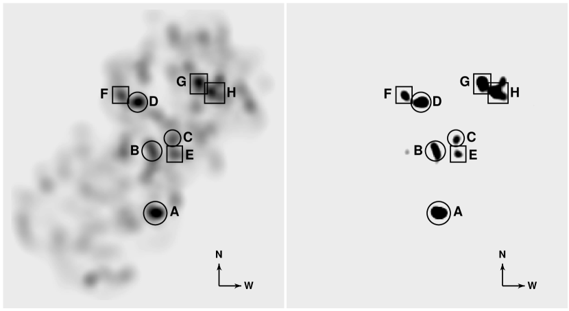
Figure 3.— Adaptive kernel density maps of galaxies meeting our color criterion in the Cl 1604 region. Previously known clusters are marked with circles. New candidates are marked with rectangles. The left panel shows the overall structure of the region. The right panel shows only areas with $\geq 14000$ red galaxies deg^-2. Each map covers a $39\hbox{$.\!\!^{\prime}$}8\times 43\hbox{$.\!\!^{\prime}$}6$ area.

Using the color-selected galaxies, we produce an adaptive kernel surface density map (Silverman, 1986; Gal et al., 2003), with $10^{\prime\prime}$ pixels and an initial smoothing window of $128^{\prime\prime}$, corresponding to 1 $h_{70}^{-1}$ Mpc at the supercluster redshift. The adaptive kernel uses a two-stage process to generate a density map. It first produces an initial estimate of the galaxy density at each point in the map using a fixed grid. It then uses this pilot estimate to apply a smoothing kernel whose size changes as a function of local density, with a smaller kernel at higher density. The smoothing size is chosen to separate the individual clusters in the supercluster without resolving much of the substructure in the clusters. The left panel of Figure 3 shows the density map for the color-selected objects from the combined LFC and COSMIC data, covering an area of $39\hbox{$.\!\!^{\prime}$}8\times 43\hbox{$.\!\!^{\prime}$}6$. The four previously detected clusters at $z\sim 0.9$ are marked with circles and labeled with the same lettering scheme as Gal & Lubin (2004). These four clusters are clearly detected as significant density peaks. However, there are a number of additional density enhancements of similar significance to the known members, especially to the northwest of the originally imaged region. To confirm that these structures are not spurious, we generated several density maps using a variety of smoothing kernels corresponding to $0.5-1.5~{}h_{70}^{-1}$ Mpc, as well as somewhat narrower and broader color cuts. Similar structures were visible in all such maps. We note the existence of numerous less significant density peaks and filaments in this map. These may be filamentary structure and possible very-low-mass systems associated with the supercluster.

The right panel of Figure 3 shows the same density map, but only pixels with red galaxy surface densities of $\geq$14,000 galaxies deg^-2 are shown. This threshold is set to include all of the spectroscopically confirmed clusters. At least four additional structures, labeled “E,” “F,” “G”, and “H”, are above this threshold. We note that this choice of threshold is subjective; as mentioned before, many other overdensities are apparent. However, the spectroscopic observations indicate that the poorest of the four confirmed clusters has a velocity dispersion of only 489 km s^-1, typical of low mass clusters (Bahcall & Cen, 1993). Therefore, the chosen density contrast will select galaxy concentrations consistent with even rather poor clusters. We also ran SExtractor on the density map with detection parameters fine-tuned to detect the four known clusters. This automated detection procedure picks up the same density peaks as those found visually.

It is unclear from this map whether E and F are unique clusters, or substructures related to the known members C and D, respectively. Unfortunately, the newly detected structures are outside the region for which we have obtained spectroscopy, so no conclusions about their independence can be drawn at this time. Similarly, G and H are very close in projection and may be components of a merging system. They are, however, clearly separated from the other supercluster members. Their nearest neighbor is over 4 $h_{70}^{-1}$ Mpc distant. Future DEIMOS spectroscopic observations are planned to determine supercluster membership for the newly discovered structures.

4. Cluster Properties

From the multicolor imaging data we are able to examine a limited number of cluster properties for each candidate. The richness is estimated by counting the number of red galaxies ($1.0\leq(r^{\prime}-i^{\prime})\leq 1.4$) in the magnitude range where both the COSMIC and LFC data are complete ($20.5\leq i^{\prime}\leq 23.5$). If all of the new candidate clusters are at the same redshift as the known ones, then this method samples the same (albeit bright) portion of the luminosity function and gives the relative richnesses of the clusters, subject to variations in the galaxy colors among the clusters. The computed richnesses, along with the cluster coordinates, are provided in Table 2. These coordinates are measured from the peaks in the red galaxy density map, and are slightly offset from the spectroscopic centers reported in Gal & Lubin (2004). The photometric and spectroscopic centers of clusters A, C, and D agree to within $1^{\prime\prime}$; the photometric center of cluster B is $\sim 30^{\prime\prime}$ (0.25 $h_{70}^{-1}$ Mpc) south of the spectroscopic center, likely because this cluster appears significantly elongated to the south. The redshifts and velocity dispersions from Gal & Lubin (2004) for the previously detected supercluster members are also given. We note that cluster C has comparable richness to three other previously known clusters, despite having a much lower velocity dispersion. This cluster was only partially imaged in the earlier survey and thus may not have complete spectroscopic coverage.

Table 2Cluster Properties

Cluster	RA	Dec	Richness	$\sigma_{los}$ (km s-1)	Redshift
A	16:04:20.9	+43:04:40.6	47	962	0.9001
B	16:04:23.6	+43:14:30.5	38	719	0.8652
C	16:04:06.5	+43:15:40.4	39	489	0.9350
D	16:04:35.7	+43:21:19.6	42	640	0.9212
E	16:04:05.0	+43:13:31.9	38	…	…
F	16:04:49.2	+43:22:19.5	37	…	…
G	16:03:45.4	+43:24:07.0	53	…	…
H	16:03:28.5	+43:24:16.5	58	…	…

We also construct CMDs for each cluster, using a circular region with radius 1 $h_{70}^{-1}$ Mpc centered on each density peak. These are shown in Figure 4,along with the combined CMD for all eight clusters. To the right of each CMD, we show the color distribution in each field as the solid histogram; this is simply the result of collapsing each CMD along the magnitude axis. For comparison, the dotted histogram shows the color distribution in a relatively blank region of the imaging data, scaled to an area with radius of 1 $h_{70}^{-1}$ Mpc. The enhancement of red cluster galaxies is clearly visible in these individual CMDs and color distributions.

Figure 4.— The $i^{\prime}$ versus $r^{\prime}-i^{\prime}$ color-magnitude diagrams within a 1 $h_{70}^{-1}$ Mpc radius for the four previously known clusters and four new candidates, as well as the eight cluster areas combined. The dashed horizontal lines indicate the color range used for cluster detection. Histograms of $r^{\prime}-i^{\prime}$ color for each cluster are plotted as the solid histogram to the right of each CMD, with the dotted histogram representing the color distribution in a blank sky region, scaled to the same area as the cluster histogram.

5. Discussion

If the red galaxy overdensities detected in this imaging survey are truly members of the Cl 1604 supercluster at $z\sim 0.9$, we have identified by far the largest known structure at redshifts approaching unity. The largest projected separation (AG) is approximately $9.6~{}h^{-1}_{70}$ Mpc, still much smaller than the apparent $93~{}h^{-1}_{70}$ Mpc depth. It appears that we have detected the southeast limit of the supercluster; no significant overdensities are visible within $\sim 10~{}h^{-1}_{70}$ Mpc directly to the east of A. We cannot rule out the structure continuing to the north/northeast or southwest. Most of the highest density peaks, including the four known clusters, are surrounded by smaller, lower density enhancements, suggesting a filamentary nature that is typical of large scale structure in simulations (Evrard et al., 2002). The large range of densities in this supercluster makes it an ideal laboratory to study the dependence of galaxy properties and their evolution on their physical environment.

We note that the apparent 8:1 axial ratio of this supercluster is comparable to or even less than that found in simulations. Shandarin et al. (2004) provide an excellent discussion of shape measurements for filaments and voids in numerical simulations with $\Lambda$CDM cosmologies, demonstrating that superclusters typically have non-trivial, highly filamentary topologies with order-of-magnitude or greater differences in the lengths of their dimensions (see their Figures 14 and 15). Furthermore, any complex filament will be easier to detect if it is viewed in projection along its longest axis. If the angular separation between the sufficiently dense regions of a supercluster becomes larger than the contiguously imaged area in a survey, then it will only be detected as a single cluster.

Our results demonstrate the efficiency of deep, moderately large area imaging in the vicinity of known clusters for detecting further structures. Hubble volume simulations show that similar superclusters are not uncommon at $z\sim 1$ (Evrard et al., 2002). Therefore, we have undertaken a wide-field imaging survey of a large sample of $z>0.5$ clusters to search for other large scale structures at these cosmologically significant redshifts. Using color cuts corresponding to early-type galaxies at a variety of redshifts we can also detect clusters at distances other than that of the target, in a manner similar to the cut-and-enhance technique of Goto et al. (2002) and the Red Sequence Cluster Survey (Gladders & Yee, 2000).

References

- Bahcall & Cen (1993) Bahcall, N. A. & Cen, R. 1993, ApJ, 407, L49
- Bertin & Arnouts (1996) Bertin, E. & Arnouts, S. 1996, A&AS, 117, 393
- Evrard et al. (2002) Evrard, A. E. et al. 2002, ApJ, 573, 7
- Faber et al. (2003) Faber, S. M. et al. 2003, Proc. SPIE, 4841, 1657
- Gal & Lubin (2004) Gal, R. R. & Lubin, L. M. 2004, ApJ, 607, L1
- Gal et al. (2003) Gal, R. R., de Carvalho, R. R., Lopes, P. A. A., Djorgovski, S. G., Brunner, R. J., Mahabal, A., & Odewahn, S. C. 2003, AJ, 125, 2064
- Gladders & Yee (2000) Gladders, M. D. & Yee, H. K. C. 2000, AJ, 120, 2148
- Goto et al. (2002) Goto, T., et al. 2002, AJ, 123, 1807
- Gunn et al. (1986) Gunn, J. E., Hoessel, J. G., & Oke, J. B. 1986, ApJ, 306, 30
- Jannuzi et al. (2004) Jannuzi, B. T., Dey, A., Brown, M. J. I., Tiede, G. P., & NDWFS Team 2004, American Astronomical Society Meeting, 204,
- Kells et al. (1998) Kells, W., Dressler, A., Sivaramakrishnan, A., Carr, D., Koch, E., Epps, H., Hilyard, D., & Pardeilhan, G. 1998, PASP, 110, 1487
- Kron (1980) Kron, R. G. 1980, ApJS, 43, 305
- Lubin et al. (2000) Lubin, L. M., Brunner, R., Metzger, M. R., Postman, M., & Oke, J. B. 2000, ApJ, 531, L5
- Postman et al. (2001) Postman, M., Lubin, L. M., & Oke, J. B. 2001, AJ, 122, 1125
- Postman et al. (1998) Postman, M., Lubin, L. M., & Oke, J. B. 1998, AJ, 116, 560
- Shandarin et al. (2004) Shandarin, S. F., Sheth, J. V., & Sahni, V. 2004, MNRAS, 353, 162
- Silverman (1986) Silverman, B. W. 1986, Monographs on Statistics and Applied Probability, London: Chapman and Hall
- Simcoe et al. (2000) Simcoe, R. A., Metzger, M. R., Small, T. A., & Araya, G. 2000, Bulletin of the American Astronomical Society, 32, 758
- Smith et al. (2002) Smith, J. A., et al. 2002, AJ, 123, 2121
- Tody (1986) Tody, D. 1986, Proc. SPIE, 627, 733
- Visvanathan & Sandage (1977) Visvanathan, N. & Sandage, A. 1977, ApJ, 216, 214