Extracting Rotational Energy in Supernova Progenitors: Transient Poynting Flux Growth vs. Turbulent Dissipation

Abstract

Observational evidence for anisotropy in supernovae (SN) may signal the importance of angular momentum and differential rotation in the progenitors. Free energy in differential rotation and rotation can be extracted magnetically or via turbulent dissipation. The importance that magnetohydrodyamic jets and coronae may play in driving SN motivates understanding large scale dynamos in SN progenitors. We develop a dynamical large scale interface dynamo model in which the differential rotation and rotation deplete both through Poynting flux and turbulent diffusion. We apply the model to a differentially rotating core surrounded by a convection zone of a SN progenitor from a initial 15$M_{\odot}$ star. Unlike the Sun, the dynamo is transient because the differential rotation is primarily due to the initial collapse. Up to $\sim 10^{51}$erg can be drained into time-integrated Poynting flux and heat, the relative fraction of which depends on the relative amount of turbulence in the shear layer vs. convection zone and the fraction of the shear layer into which the magnetic field penetrates. Both sinks can help facilitate explosions and could lead to different levels of anisotropy and pulsar kicks. In all cases, the poloidal magnetic field is much weaker than the toroidal field, and the Poynting flux is lower than previous estimates which invoke the magnitude of the total magnetic energy. A signature of a large scale dynamo is that the oscillation of the associated Poynting flux on $\sim 1$ sec time scales, implying the same for the energy delivery to a SN.

(submitted to New Astronomy)

Key Words: supernovae: general – stars: magnetic fields – stars: neutron – MHD – dynamo theory–Gamma rays: bursts

1 Introduction

Observations suggest that many supernovae (SN) are intrinsically anisotropic. As summarized by Wheeler (2004a,b) evidence comes from: (1) bipolar structure in supernova remnants (Dubner et al. 2002); (2) optical jet and counter jet structures in Cas A (Fesen 2001); (3) X-ray jets and toroidal emission of intermediate mass elements (Hughes et al. 2000; Hwang, Holt, Petre 2000; Willingale et al. 2002); (4) asymmetric ejecta in SN1987A perpendicular to the major axis of the rings ((Wang et al. 2001, 2002); and (5) Optical polarization in both Type I and Type II supernovae (see Wang 2004 for a review) with the Type Ib,c polarization being higher than that of Type II (Wang et al. 1996; Wang et al. 2001), but with the latter increasing with time (Wang et al. 2001; Leonard et al. 2001). Since Type I SN represent a naked core, and the core at late times in Type II becomes exposed, a consistent interpretation is that the SN engine is a source of this asymmetry. At minimum, anisotropy likely reveals the role of rotation in SN engines and the need to incorporate non-spherically symmetric physics.

1.1 Magnetic Fields

The combination of rotation, highly ionized plasma, stratified turbulence, and magnetic fields has prompted various considerations of MHD outflows as a source of this asymmetry, if not the source of the SN explosion itself. Recent renewed interest in proposals relating MHD outflows to supernovae (Leblanc & Wilson 1970; Meier et al. 1976; Ardeljan, Bisnovatyi-Kogan, & Moiseenko 1998; Khokhlov et al. 1999; Wheeler et al. 2000; Wheeler, Meier, & Wilson 2002; Moiseenko, Bisnovatyi-Kogan, & Ardeljan 2004) is bolstered by the observational association of SN with Gamma-ray bursts (Galama et al 1998; Iwamoto et al. 1998; Stanek et al. 2003; Hjorth et al. 2003; Thomsen et al. 2004; Cobb et al. 2004 Gal-Yam et al. 2004; Malesani et al. 2004). MacFadyen, Woosley, & Heger 2001). That magnetized outflows have also long been thought to be important in young stellar objects, active galactic nuclei, pulsar winds, and microquasars (of which GRB are likely one class) suggests that explosive bipolar outflows in astrophysics may all involve some combination of rotation and magnetic fields.

Previous work on magnetic field amplification in pre-supernovae core conditions have employed either (i) simple shear that grows toroidal field linearly (e.g. Leblanc & Wilson 1970; Ardeljan, Bisnovatyi-Kogan, & Moiseenko 1998; Wheeler 2000), (ii) traditional kinematic convective $\alpha-\Omega$ dynamo models to grow ordered fields (Thompson & Duncan 1993), which in principle grow large-scale fields exponentially, or (iii) the exponential field growth from the magneto-rotational instability (MRI, e.g. Balbus & Hawley 1998) (Akiyama et al. 2003; Moiseenko et al. 2004), whose saturated magnetic energy was used as a rough estimate for the large-scale toroidal field. Each has its merits and its limitations. In the presence of turbulent diffusion, (i) will not sustain the field. The approach of (ii) offers exponential growth and is an important step forward, but the backreaction of the field on the driving flow, the separate generation of toroidal vs. poloidal fields, and the spatial location of the $\alpha$ and $\Omega$ effects still need to be determined. The recent approach of Akiyama et al. in (iii) offers a useful model of the internal and rotational structure of the inner SN engine, and also makes careful estimates of the saturated energy of the magnetic field adopted from results obtained in MRI disk simulations. Whether these values also apply to pressure-supported stars remains to be studied in detail because the MRI likely transports angular momentum on spherical shells (Balbus & Hawley 1994), not radially; the latitudinal differential rotation may be most important. If 3-D turbulence develops, then field amplification will take place from the MRI. Moiseenko et al. (2004) provide 2-D simulations of what appear to be MRI-driven SN, starting from a relatively strong, ordered poloidal field. However, in 2-D, there is not sustained dynamo action to amplify the total magnetic energy from arbitrarily small values.

An important question is whether a magnetically driven outflow requires a large-scale field in the supernova progenitor engine. By large-scale field, we mean one that maintains the sign of its flux over many dynamical times, when averaged over the size of the engine region. Large-scale fields are helpful, if not necessary, in generating outflows in disks or stellar coronae, and perhaps by analogy, also in SN engines. If the field needs to buoyantly rise above the dynamo region to a height at which it provides the dominant contribution to the stress, the field should be of large enough scale to avoid being shredded by turbulence. Once at the region where it dominates, the field can further relax to even larger scales. Comparing the shapes of observed outflows to those from theoretical studies (e.g. Moiseenko et al. 2003) may help determine the relative importance of large scale fields vs. a simple magnetic pressure gradient.

This magnetic field may drive a “jack-in-the-box” type of magnetic spring explosion. (In addition to Wheeler, Meier, & Wilson (2002), see also Matt et al. (2004) for simulations of a magnetic explosion without specifying the field origin, and Moiseenko et al. (2004) for a magnetic explosion driven SN.). The potential efficacy of magnetically-driven outflows for SN is evident from recent work by Moiseenko et al. (2004). However, as in the magnetic explosion of Matt et al (2004) for planetary nebulae, Moiseenko et al. (2004) start with a significant large-scale poloidal field, comparable in strength to the saturated poloidal field whose growth we will study here from an initially small seed field. Any dynamo driven outflow must occur while the dynamo is active because afterward the field decays.

Large-scale field generation does not exclude the presence of the MRI: When the MRI operates in a stratified medium, it may provide a source of helical turbulence that allows one sign of magnetic helicity to migrate to large scales, producing large-scale magnetic fields (e.g. Brandenburg et al. 1995; Blackman & Tan 2004) or a helicity flux (Blackman & Field 2000; Vishniac & Cho 2001). In our large scale dynamo herein, the source of helical turbulence is considered to be convection driven by shock heating and neutrino deposition rather than the MRI, though the particular source is not essential for our calculations. It should also be emphasized that studies focusing on magnetic energy amplification from the MRI (Balbus & Hawley 1998) typically study growth of the total magnetic energy (e.g. Akiyama et al. 2003) rather than a specifically large-scale field in the sense we have defined above. The backreaction of the field on the shear is not usually considered in MRI studies.

Note that instead of a bulk dynamical influence of large scale fields, Ramirez-Ruiz and Socrates (2004) highlight an alternative role facilitated by large scale fields that buoyantly rise to form a corona. They suggest that such a corona could distribute the binding energy dissipation such that the neutrino spectrum becomes non-thermal. This increases the efficiency of neutrino-matter coupling by an order of magnitude. The SN would be neutrino driven, but symbiotically dependent on a corona.

1.2 Turbulent Viscosity

Magnetic fields generated in situ are amplified by extraction of the free energy in differential rotation. Thompson et al. (2001) point out that the energy lost into heat via turbulent damping of the shear supplies enough energy when combined with neutrino driving to create a SN explosion. The energy lost from the shear to heat represents a conversion of some of the binding energy into a form more efficiently coupled to the matter than neutrinos. In the presence of turbulence (which itself could be induced by the magnetic field) a competition emerges between draining the shear into Poynting flux vs. heat. Both sinks may help drive SN in different ways.

1.3 What We Do Here

Here we study the dynamical evolution of differential rotation and large scale magnetic field growth with several key new features: 1) we explicitly consider the backreaction of the magnetic field on the shear and rotation driving the field growth and 2) allow the shear and rotation to deplete via Poynting flux and turbulent dissipation. The latter turns out to be important and a key result of our study is to show the relative depletion into each channel.

We derive a dynamical generalization of the large-scale interface dynamo proposed by Parker (1993) for the Sun (see also Charbonneau & MacGregor 1997; Markiel & Thomas 1999; Zhang et al. 2003). Interface dynamos differ from the original $\alpha-\Omega$ dynamos in that the dominant region of shear and the dominant region of helical turbulence are not co-spatial. The shear associated with differential rotation is concentrated in a layer (the $\Omega$-layer) lying beneath the turbulent convection zone (the $\alpha$ layer). Such a scenario has been a leading model for the solar dynamo, and has also been applied to white dwarfs (Markiel, Thomas & Van Horn 1994; Thomas, Markiel & Van Horn 1995) and to AGB stars (Blackman et al. 2001). In all of these cases, helical turbulence in the convective zone provides the dynamo $\alpha$ effect and thus generates the poloidal field. Turbulent pumping (e.g. Tobias et al. 2001) pushes the poloidal field downward into the strong shear layer where the toroidal field is amplified. The rotational and convective environment of the proto-supernova engine in core-collapse supernovae has a similar structure, with a strong shear layer surrounded by a convective envelope. However, unlike the sun where the differential rotation profile is re-established by convection, in the SN context the intial shear decays dynamically as the field grows. Whether or not convection may refuel the differential rotation needs further study, but here we assume that the dominant source of differential rotation is that from the initial collapse. This differential rotation will deplete as the field is amplified or as the shear is damped by turbulence. We explicitly include the dynamical evolution of the shear and rotation in addition to that of the magnetic field, unlike previous work. The dynamo becomes transient in the SN progenitor.

Dynamo research must accommodate two competing needs: the need for a theory that rigorously includes the backreaction of the growing magnetic field on the flow, and the need to model the field growth in a realistic system. Meeting these two goals is difficult both analytically and numerically, and compromises must be made on both fronts. Our aim here is to develop a transient large scale dynamo model and apply it to the SN progenitor context as simply as possible, while still including the time-dependent nonlinear dynamical quenching of the shear and rotation.

In section 2 we present the dynamical equations for the magnetic field, shear, and rotation. In section 3 we discuss the parameter choices and present the corresponding solutions. In section 4 we discuss the implications of the calculated Poynting flux and the fractional shear energy drained into magnetic energy vs. heat. We conclude in section 5 and identify some unresolved issues for future work.

2 Transient Interface Dynamo and Velocity Equations

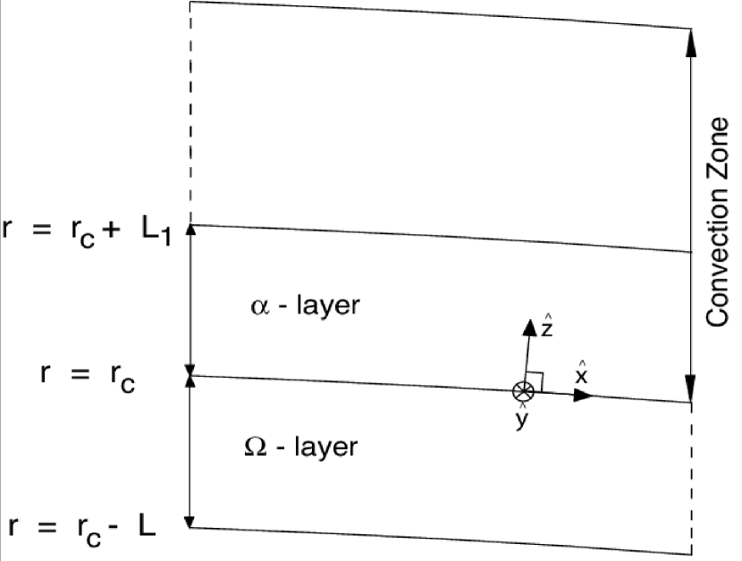
Figure 1: Schematic meridional slice of the spherical dynamo engine. The local Cartesian coordinate system is shown. The $\alpha$-effect occurs in a layer of thickness $L_{1}$ equal to the local density scale height at the base of the convection zone ($r=r_{c}$). The $\Omega$-effect occurs in a concentrated region of thickness $L$ which extends from the surface of the NS to the base of the convection zone.

We generalize the interface dynamo model of Markiel, Thomas & Van Horn (1994) to include the dynamical evolution of shear, rotation, and Poynting flux. The concept of the interface dynamo is illustrated in the meridional slice shown in Fig. 1. Two distinct regions adjoin at the interface radius $r=r_{c}$. In the inner region, the differential rotation (the $\Omega$ effect) wraps the poloidal field into a toroidal field with the rotation profile initially varying linearly from $\Omega$ at $r=r_{c}$ to $\Omega+\Delta\Omega$ at $r=r_{c}-L$, where $\Delta\Omega$ measures the differential rotation. The values of the quantities at the initial time of the calculation are indicated by a subscript $0$, that is $\Omega_{0},$ and $\Delta\Omega_{0}$. The outer layer, representing the convection zone, rotates rigidly with angular velocity $\Omega_{0}$. There, cyclonic convection (the $\alpha$-effect) converts toroidal field into poloidal field. This poloidal field is then pumped or diffused downward into the $\Omega$ layer where the shear again further amplifies the toroidal field. The relevant $\alpha$ layer has thickness $L_{c}$, which corresponds to a density scale height from the base of the convection zone. A full treatment of the interface dynamo would include anisotropic diffusion, stratification and shear, global 3-D treatment of the convection, self-consistent buoyancy dynamics, self-consistent sustenance of $\alpha$ and a dynamical treatment of the non-linear backreaction of magnetic field on the velocity field. We provide a minimalistic approach that incoporates some of these ingredients in a 1-D model to illustrate the mechanism simply.

2.1 Magnetic Field Evolution

To solve for the magnetic field, we employ the mean-field induction equation, derived by averaging the induction equation in the presence of helical velocity fluctuations. The standard mean field induction equation, ignoring cross-helicity, is (e.g. Parker 1979)

$$\partial_{t}\overline{\bf B}=\nabla{\times}\langle{\bf v}\times{\bf b}\rangle+\nabla{\times}(\overline{\bf V}\times\overline{\bf B})+\lambda\nabla^{2}\overline{\bf B}=\nabla{\times}(\alpha\overline{\bf B})+\nabla{\times}(\overline{\bf V}\times\overline{\bf B})-\nabla{\times}(\beta_{{\bf i}}\nabla{\times}\overline{\bf B})+\lambda\nabla^{2}\overline{\bf B},$$ (1)

where $\overline{\bf B}$ is the mean field, $\overline{\bf V}$ is the mean velocity, $\lambda$ is the turbulent diffusivity, and the turbulent electromotive force is $\langle{\bf v}\times{\bf b}\rangle=\alpha\overline{\bf B}-\beta_{{\bf i}}\nabla{\times}\overline{\bf B}$, where $\alpha$ is the pseudoscalar helicity dynamo coefficient and $\beta_{i}$ is a turbulent magnetic diffusivity, where the index allows different values for the poloidal and toroidal field equations. Although we have in mind a spherical system, for present purposes we simplify the analysis by working in local Cartesian coordinates. Simplified versions of the equations we invoke for the mean magnetic field have been used in previous interface dynamo models (Robinson and Durney (1982); Markiel, Thomas, & Van Horn (1994)) without adequate derivations, and so we present a full derivation here. The coordinates are shown in Fig. 1. Writing $\overline{\bf A}=(\overline{A}_{x},\overline{A},\overline{A}_{z})$ and assuming that (i) the mean fields are axisymmetric (i.e. $\partial_{y}\overline{\bf M}=0$ for any mean quantity $\overline{\bf M}$), (ii) $\overline{\bf V}=(0,\overline{V},u)$, (iii) $\overline{\bf B}=(0,\overline{B},\partial_{x}\overline{A})$ (so $\partial_{z}\overline{A}=0$) (iv) $\beta_{{\bf i}}=\beta_{p}$ for the poloidal field equation and $\beta_{{\bf i}}=\beta_{t}$ for the poloidal field equation and $\nabla\beta_{t}=\nabla\beta_{p}=0$. (v) $\beta_{{\bf i}}>>\lambda$ we can write the equations for the toroidal magnetic field $\overline{B}$ and the vector potential $\overline{A}$ as

$$\partial_{t}\overline{B}=-\alpha\partial_{x}^{2}\overline{A}-\partial_{z}\alpha\partial_{x}A+\partial_{x}\overline{A}\partial_{z}\overline{V}-u\partial_{z}\overline{B}-u\overline{B}/L+\beta_{t}\nabla^{2}\overline{B}$$ (2)

$$\partial_{t}\overline{A}=\alpha\overline{B}+\beta_{p}\partial_{x}^{2}\overline{A},$$ (3)

where we have used $-\overline{B}\partial_{z}u\sim-u\overline{B}/L$ which we take as a loss term due to magnetic buoyancy with $u>0$. If we assume that the Fourier transform of the field is proportional to a $\delta$ function in wavenumber (i.e. the mean field has a single large scale), then we can write $\overline{A}=A(t)e^{(ik_{x}x+ik_{z}z)}$ and $\overline{B}=B(t)e^{(ik_{x}x+ik_{z}z)}$, where $A(t)$ and $B(t)$ are complex-valued functions. Then, assuming the $\partial_{z}\alpha$ term to be small, Eqs. (2) and (3) become

$$\partial_{t}B\simeq\alpha k_{x}^{2}A-ik_{x}r_{c}A{\Delta\Omega\over L}-iuk_{z}B-uB/L-\beta_{t}k^{2}B$$ (4)

$$\partial_{t}A=\alpha B-\beta_{p}k^{2}A,$$ (5)

where $k^{2}=k_{x}^{2}+k_{z}^{2}$, and we have used

$$\partial_{z}\overline{V}\sim-r_{c}\Delta\Omega/L$$ (6)

to obtain the third term in (4), based on the interface geometry shown in Fig. 1. We write

$$\beta_{t}=c_{t}{v}L\ \ \ {\rm and}\ \ \ \beta_{p}=c_{p}{v}L$$ (7)

where $c_{t},c_{p}$ are distinct dimensionless constants that allow our 1-D model to account for the fact that toroidal and poloidal fields are generated in separate regions with distinct turbulent diffusivities. The quantity $v_{1}$ is a typical convective velocity at the middle of the $\alpha$ layer (i.e. at $r=r_{c}+L_{1}/2$, see Fig. 1).

In interpreting $-\frac{uB}{L}$ as the rate of loss of toroidal flux due to the buoyant rise of toroidal flux out of the dynamo region, we use the expression for the rise velocity of a flux tube (Parker 1955, 1979), namely

$$u=\frac{3Q}{8}{\left(\frac{a}{L}\right)}^{2}\frac{|\overline{B}|^{2}}{4\pi\rho{v}}=\frac{3Q}{32}\frac{\overline{V}_{A}^{2}}{v},$$ (8)

where $a$ is the radius of the flux tube (assumed to be $L/2$), $\overline{V}_{A}$ is the Alfvén speed associated with $\overline{B}$, and $Q$ is a dimensionless constant.

2.2 Quenching of $\alpha$

While there is no compelling evidence that $\beta$ is catastrophically quenched in convective 3-D MHD turbulence, recent work on dynamo theory has shown that $\alpha$ quenching can be understood dynamically via magnetic helicity conservation (e.g. Blackman & Field 2002; Brandenburg & Subramanian 2004 for a review). The build-up of the large-scale field is associated with a build-up of the large-scale magnetic helicity, $\overline{\bf A}\cdot\overline{\bf B}$. In the absence of boundary terms, magnetic helicity is well conserved, and the small-scale helicity builds up to equal magnitude but opposite in sign to that of the large scale. Since $\alpha$ depends on the difference between kinetic and current helicities, the build up of small-scale magnetic (and thus current) helicity eventually saturates the dynamo. If boundary terms can allow for a helicity flux (Blackman & Field 2000; Vishniac and Cho 2001) then the $\alpha$ quenching is alleviated but at the expense of a lower saturated mean field (Blackman & Brandenburg 2003). If the small-scale helicity can be preferentially removed then the large-scale growth proceeds longer to larger values. Shear may also reduce the impact of $\alpha$ quenching (Brandenburg & Sandin 2004). Shear also leads to anisotropic turbulence and possibly a shear-current dynamo (Rogachevskii & Kleeorin 2003), though we do not presently discuss this further.

Here we are interested in demonstrating the most basic aspects of a transient large scale dynamo and adopt a parameterization of the $\alpha$ effect backreaction that can be used to approximate the non-linear quenching. We modify the quenching formula used for previous interface dynamos (Markiel, Thomas, & Van Horn (1994)) to also facilitate the coupling of $\Omega$ quenching into $\alpha$. We write

$$\alpha=\alpha_{0}(\Omega/\Omega_{0})^{q}{Exp}\left[-\gamma_{1}{\frac{\overline{B}^{2}/8\pi}{\rho_{1}v_{1}^{2}/2}}\right],$$ (9)

where $\gamma_{1}$ is a dimensionless constant, $\rho_{1}$ and $v_{1}$ are the mass density and a typical convective velocity at the middle of the $\alpha$ layer. We assume $q=1$ which so that $\alpha$ quenching is coupled to the $\Omega$ quenching discussed below, and use (Durney & Robinson (1981))

$$\alpha_{0}=c_{\alpha}\frac{L_{1}^{2}\Omega_{0}}{r_{c}},$$ (10)

where $0<c_{\alpha}<1$ is a dimensionless constant.

2.3 Evolution of $\Delta\Omega$ and $\Omega$

The amplification of the field and turbulent diffusion will drain the differential rotation and Poynting flux drains some of the remaining rotational energy until the dynamo shuts off. We must therefore construct dynamical equations for $\Delta\Omega$ and $\Omega$.

If we ignore second derivatives in space, using (6) we can write the differential equation for the shear at $r=r_{c}$ as

$$-\partial_{t}(r_{c}\Delta\Omega)=\partial_{t}(\overline{V}_{y}(r_{c})-\overline{V}_{y}(r_{c}-L))\simeq\partial_{t}(L\partial_{x}\overline{V}_{y}).$$ (11)

To obtain the desired differential equation for the right hand side, we subtract the time dependent differential equations for the velocity at $r_{c}$ and $r_{c}-L$. From the Navier-Stokes equation for the mean velocity and the assumption that gradients in the $y$ direction vanish,

$$\partial_{t}\overline{V}_{y}=-\overline{\bf V}\cdot\nabla\overline{V}_{y}+{1\over 4\pi\rho}(\overline{\bf B}\cdot\nabla)\overline{B}_{y}+\nu\nabla^{2}\overline{V}_{y}\simeq{1\over 4\pi\rho}\partial_{x}\overline{A}\partial_{z}\overline{B}_{y}+\nu(\partial_{x}^{2}+\partial_{z}^{2})V_{y},$$ (12)

where $\nu$ is a turbulent viscosity. From Eqs. (11) and (12) we then have

$$\begin{array}[]{r}\partial_{t}(r_{c}\Delta\Omega)=({1\over 4\pi\rho}\partial_{x}\overline{A}\partial_{z}\overline{B}_{y}+\nu(\partial_{x}^{2}+\partial_{z}^{2})v_{y})|_{r_{c}}-({1\over 4\pi\rho}\partial_{x}\overline{A}\partial_{z}\overline{B}_{y}+\nu(\partial_{x}^{2}+\partial_{z}^{2})v_{y})|_{r_{c}-L}\\ \simeq{L\over 4\pi}\partial_{z}{1\over\rho}\partial_{x}\overline{A}\partial_{z}\overline{B}_{y}+\nu{L}(\partial_{z}\partial_{x}^{2}+\partial_{z}^{3})v_{y}\\ \simeq{L\over 4\pi}\left[{1\over\rho}(\partial_{z}\partial_{x}\overline{A}\partial_{z}\overline{B}_{y})_{r_{c}}+(\partial_{x}\overline{A}\partial_{z}^{2}\overline{B}_{y})_{r_{c}}-({\partial_{z}\rho\over\rho^{2}}\partial_{x}\overline{A}\partial_{z}\overline{B}_{y})_{r_{c}}\right]-\frac{\nu{r_{c}}}{L^{2}}\Delta\Omega.\end{array}$$ (13)

Taking $\partial_{z}\rho\sim(\rho_{2}-\rho_{1})/L$, where $\rho_{2}$ and $\rho_{1}$ are the densities at the inner and outer boundaries of the shear layer, and using $\overline{A}=A(t)e^{i(k_{x}x+k_{z}z)}$ and $\overline{B}=B(t)e^{i(k_{x}x+k_{z}z)}$ as in the derivation of Eqs. (4) and (5), we then obtain

$$\partial_{t}\Delta\Omega={L\over 4\pi r_{c}\rho}\left[-k_{x}k_{z}^{2}\rho(Re(\overline{A})Re(i\overline{B})+Re(i\overline{A})Re(\overline{B}))-\partial_{z}\rho k_{x}k_{z}Re(i\overline{A})Re(i\overline{B})\right]-\frac{\nu}{L^{2}}\Delta\Omega.$$ (14)

As stated above, we also need an equation for the time evolution of $\Omega(t)$. We obtain this equation by noting that the rotational energy of the field-anchoring matter is drained by the Poynting flux. The Poynting flux at $r_{c}$ is given by

$$L_{mag}={c\over 4\pi}\int{\overline{\bf E}}\times{\overline{\bf B}}\cdot d{\bf S}_{c}\simeq{1\over 4\pi}\int\Omega r_{c}Re(\overline{B}_{z})Re({\overline{B}}_{y})\cdot d{\bf S}_{c}\simeq-Re(\overline{B}_{z})Re(\overline{B}_{y})\Omega r_{c}^{3}.$$ (15)

Calculating this quantity requires the separate determination of the toroidal and poloidal magnetic fields: because these components can be out of phase, the maximum Poynting flux is not simply the product of their respective maxima. We approximate the total rotational energy in the shear layer as the kinetic energy of the of mass $M\simeq 10^{34}$g of the shear layer. moving with the velocity of the outer boundary, namely, $E_{rot}\sim Mr_{c}^{2}{\Omega}^{2}/2$. This value is imprecise but gives between $10^{51}\leq E<10^{52}$, which is consistent with other estimates of the available rotational energy (Thompson et al. 2005). However, because the fields may not penetrate into the entire shear layer, we allow for the fact that only a fraction of the rotational energy may be available for conversion into Poynting flux. We account for this reduced available rotational energy by multiplying $E_{rot}$ by $\delta/L$, where $\delta$ is the depth penetrated by the field into the shear layer, a quantity will derive in (20) below. In combination with Eq. (15), the time derivative of the rotational energy then leads to the time-evolution equation for $\Omega$

$$\partial_{t}\Omega\simeq{Re(\overline{B}_{z})Re(\overline{B}_{y})r_{c}\over M\delta}$$ (16)

Eqs. (4), (5), (14) and (16), are the coupled differential equations to be solved for the transient large scale interface dynamo. In all solutions discussed below, we will take $\beta_{t}=\nu$, and define the the poloidal turbulent magnetic Prandtl number

$$P_{M,p}\equiv\frac{\nu}{\beta_{p}}=\frac{\beta_{t}}{\beta_{p}}.$$ (17)

The role that $P_{M,p}<1$ plays is very important: Although the equations we solve are 1-D, we invoke our use of $P_{M,p}<1$ is a simple way of capturing aspects of a 2-D interface dynamo. In particular, in a realistic progenitor the shear layer is convectively stable and thus can be expected to have a lower turbulent diffusion coefficient than the convective zone. In addition, the toroidal field is primarily amplified in the shear layer where as the poloidal field is primarily amplified in the convection zone. We therefore take $\beta_{p}>>\beta_{t}=\nu$.

3 Discussion of Solutions

3.1 Kinematic Solution

For the relevant parameters, the first term on the right of (4) is small compared to the next term, implying that we are initially in the $\alpha-\Omega$ interface dynamo regime. It is useful to first consider the kinematic limit, $\gamma_{1}=q=0$, $\partial_{t}f=\partial_{t}\Omega=0$, which allows us to determine the conditions for initial growth of the dynamo field. In this case, (4) and (5) are the only equations to be solved. Assuming that $k_{z}<<k_{x}$, there are then exponentially growing solutions of the form $A(t)=A_{0}e^{nt}$ and $B(t)=B_{0}e^{nt}$, such that $\overline{A}=Re(A_{0}e^{nt+ikx})$ and $\overline{B}=Re(B_{0}e^{nt+ikx})$, and

$$Im(n)=\left({\alpha_{0}\Delta\Omega kr_{c}\over 2L}\right)^{1/2}.$$ (18)

The amplitude of these waves grows (i.e. $Re(n)>0$) only when the initial dynamo number

$$N_{D,0}\equiv N_{D}(0)=\frac{\alpha_{0}kr_{c}\Delta\Omega_{0}}{2L\beta_{t}\beta_{p}k^{4}}=\frac{\alpha_{0}kr_{c}\Delta\Omega_{0}}{2LP_{M,p}\beta_{p}^{2}k^{4}}$$ (19)

exceeds unity. This kinematic solution will provide insight into the non-linear solutions.

3.2 Penetration Depth

In our solutions below, we will consider cases in which the entire differential rotation layer is available for magnetic field amplification but also cases in which only a fraction $\delta/L$ of the layer is available. The estimate of $\delta$ for the latter case is obtained by considering it to be the distance that the toroidal field can diffuse into the shear layer during a cycle period. The cycle period does increase during the dynamical regime, but as a lower limit we use the kinematic value obtained from the inverse of (18) namely $\tau=2\pi(\frac{2L}{\alpha_{0}\Delta\Omega_{0}kr_{c}})^{\frac{1}{2}}$. We then have

$$\delta\simeq(\beta_{t}\tau)^{\frac{1}{2}}.$$ (20)

3.3 Nonlinear Solutions for SN Progenitors

Table 1 and Figs. 2-5 represent example solutions of Eqs. (4), (5), (14) and (16). We discuss the choices of parameters and the meaning of these solutions below.

For the engine structure, we employ the profiles of Akiyama et al. (2003) for a rapidly rotating neutron star (NS) formed from the collapse of a 15 $M_{\odot}$ progenitor. These authors used a 1-D stellar evolution code to obtain the radial structure of a spherical core collapse, and then computed the rotational velocity profiles a posteriori by assuming that angular momentum is conserved on spherical shells during the collapse. We adopt the values of the density and rotation profiles corresponding to 384 milliseconds after bounce. While Akiyama et al. (2003) used their structure and rotation solutions as inputs for their MRI dynamo calculations, we use these inputs for the interface dynamo of the previous section.

Using the characteristic numbers, our differential rotation layer ($\Omega$-layer, Fig. 1) extends down to the surface of the NS ($r_{c}-L=1.5\times{10^{6}}$ cm) and the base of the convection zone is located at $r_{c}=4\times{10^{6}}$ cm. We take the $\alpha$ effect to occur above the base of the convection zone in a layer whose thickness ($L_{1}=2.3\times{10^{6}}$ cm) equals the local density scale height. The density in the middle of the $\Omega$ layer is taken to be $\rho_{2}=2.4\times{10^{13}}$ g/cm³ and that of the $\alpha$-layer is taken to be $\rho_{1}=2.4\times{10^{12}}$ g/cm³ (Akiyama et al. 2003). A typical convective velocity (e.g. Herant et al. 1994) of $v_{1}=10^{8}$ cm/s is taken in the middle of the $\alpha$ layer and is sustained by the neutrino luminosity and lepton gradients. The interface dynamo equations of the previous section contain the dimensionless constants $\gamma_{1}$, $c_{t}$, $c_{p}$, $c_{\alpha}$, and $Q$. For the $\alpha$ quenching parameter, $\gamma_{1}$, we take $\gamma_{1}=0.1$, for which the solutions turn out to be $\Omega$-quenching limited. Regarding the parameters $c_{t}$, $c_{p}$, $c_{\alpha}$, and $Q$, we note that the dynamo number is sensitive only to the ratio $c_{\alpha}/c_{t}c_{p}$, whereas $Q$ enters in the buoyancy loss term and $c_{\alpha}$ enters in the kinematic dynamo frequency. A range of choices can be considered to be appropriate given the uncertainty in the detailed properties of the turbulence, but, in the spirit of mixing-length theory, we choose values similar to those which yield dynamo solutions matching the solar dynamo period and field strength when the theory (without $\Omega$ and $\Delta\Omega$ quenching) is applied in that context (Markiel, Thomas, & Van Horn (1994)).

The magnetic field strengths $\overline{B}_{x},\overline{B}_{y}$ are computed at the interface layer ($r=r_{c}$). At $r=r_{c}$, $x=r_{c}\theta$ locally where $\theta$ is the poloidal angle from the prescribed $z$ axis in Fig. 1. Although the Cartesian approach technically applies only locally, we choose the mode that most closely corresponds to dipole symmetry, namely that for which $k_{x}r_{c}=2$.

Fig. 2 shows the poloidal field, toroidal field, Poynting flux, $\Omega$, $\Delta\Omega$, and a comparison of the time-integrated Poynting flux compared to the energy in the differential rotation lost to turbulent dissipation for the parameter row 7 in Table 1. For Fig. 2 we used (20) for $\delta$. Note that the cycle period of the field growth is reflected in the oscillations of the Poynting flux in the upper left panel. The fact that the dotted curve is above the solid curve in the upper right panel indicates that for this set of paramters, more of the free energy is drained into heat via turbulent dissipation rather than into Poynting flux.

Fig. 3 is similar to Fig. 2 but with parameters used from row 4 in Table 1. The same $\beta_{p}\propto c_{p}$ is used as in Fig. 2 but a lower $\beta_{t}\propto c_{t}$ is used and corresponding to a lower $Pr_{M,p}$. From (19) we see that $N_{D}$ increases which implies shorter cycle period and a shorter time for the field to saturate compared to Fig. 2. A smaller $\beta_{t}$ and shorter cycle period accounts for the lower $\delta/L$ compared to Fig. 2, but a lower $\beta_{t}$ also implies less diffusion in the equation for $B_{\phi}$ so $B_{\phi}$ peaks at a larger value than in Fig. 2.

In Figs. 4 and 5 we show the cases of rows 17 and 18 in Table 1 respectively. For these cases when computing the evolution of the total rotational energy, we set $\delta=L$ to compare with Figs. 2-3 where (20) was used. In both of these cases, the total integrated Poynting flux exceeds the energy lost in the shear layer via turbulent diffusion. The difference between Figs 4 and 5 is the buoyancy constant $Q$ which is smaller in Fig. 5 than in Fig. 4.

Table 1 shows a variety of other cases not shown in the figures, but which can be analyzed similarly. One point to note, which is evident from (19) is that the growth rate dependents indepently on $Pr_{M,p}$ and $\beta_{p}$ (or equivalently, $c_{p}$ and $c_{t}$) so that a fixing $Pr_{M,p}$ alone does not fix the saturation values. This can be seen e.g. by comparing rows 4 and 5 of Table 1.

Taken collectively, the figures and Table 1 illustrate the transient nature of the dynamo. The transience and saturation are due to the depletion of $\Delta\Omega$ and $\Omega$. The former depletes due to field amplification and turbulent diffusion and $\Omega$ depletes from the Poynting flux. Most dynamo calculations in main sequence stellar contexts and accretion disks ignore $\Delta\Omega$ and $\Omega$ quenching and decay. In the present SN progenitor context the dynamical evolution of these quantites is important. When $\Delta\Omega$ and $\Omega$ are enforced as constant, $\alpha$ quenching and buoyancy would determine the maximum amplitudes of the field and Poynting flux. In that case, the curves analagous to Figs. 2-5 would asymptote to oscillating curves of constant peak amplitudes.

Increasing $\Delta\Omega_{0}$ and $\Omega_{0}$ increases the initial dynamo number $N_{D}$. This increases the rate of growth and maximum value of the fields obtained, However, due to the finite amount of rotational energy, estimated above (16), a faster growing dynamo lasts a shorter time. This can also be seen by comparing Figs 2 and 3. The latter has a faster growth to a higher peak, but decay from the peak is faster. That $\Delta\Omega$ and $\Omega$ do not fall to $0$ before the field decays in all of the figures results because the effective dynamo number becomes sub-critical well before all of the rotational energy is drained.

The oscillation periods of the toroidal and poloidal fields are roughly consistent with $2\pi/Im(n)$ at early times until the rise to the first maximum peak. During this time, the Poynting flux oscillates with a period half that of the these field components. After the field and Poynting flux rise to their absolute maxima, the cycle period increases slightly. This increase occurs because the cycle period in Eq. (18) is $\propto\Omega^{-1/2}\Delta\Omega^{-1/2}$, and the dynamical quenching of $\Delta\Omega$ and $\Omega$ thus increase the period. Only a modest decrease in $\Omega\Delta\Omega$ makes the dynamo number subcritical, after which the field decays.

The notches that occur in the decay of the rotational quantities in Figs. 2-5 occur during the phase of each cycle when the field is well away from its peak in amplitude. At these times, the damping of the differential rotation and rotation is weak, and their rapid decay is arrested. Note that the Poynting flux drops below zero during part of the field oscillations (see the top left panels in Figs. 2-5), and so the rotational quantities can even slightly increase during that time. This effect is small and for the most part the curves represent decay to the values at which the dynamo number drops below the critical value for growth.

4 Further Implications

4.1 Cycle Period as a Signature of Magnetic Influence

If signatures of the time dependence of energy injection to SN could be constrained observationally, the quasi-periodicity seen in the Poynting flux would be a specific prediction of the influence on a large scale dynamo. Similarly, were a Poynting-flux driving cycle to operate in GRB progenitors, one might consider this to provide a source of variability. Even if the role of magnetic fields is to supply a corona as needed in Ramirez-Ruiz & Socrates (2005) rather than for directly driving an outflow, evidence for the cycle period could still be present. However, only when $\beta_{t}<<\beta_{p}$ can the Poynting flux be a competitive sink of the free energy compared to the turbulent dissipation. When the latter is the primary sink, the SN explosion can still be strongly aided, as emphasized in Thompson et al. 2005, but neither evidence for a cycle period nor significant anisotropy would necessarily be expected.

4.2 Pulsar kicks

If a significant source of energy for the SN is rotational energy of the shear layer (or the NS), then only a small fraction of it needs to be asymmetrically extracted across the poles to produce pulsar kicks of $\sim 200$km/s. To see this, note that the estimated kick kinetic energy $E_{k}$ compared to that available in $E_{PF}$ The ratio for a $1.4M_{\odot}$ neutron star is

$$K={E_{k}\over E_{PF}}\simeq 0.01\left({v_{k}\over 200{\rm km/s}}\right)^{2}\left(E_{PF}/E_{rot}\over 0.1\right)^{-1}\left(E_{mag}\over 10^{51}\right)^{-1}$$ (21)

where the integrated Poynting flux $E_{PF}$ is scaled to typical values for or 15$M_{\odot}$ progenitor. That $K<<1$ is favorable as it implies a weakly asymmetric bipolar outflow can drive the kick. This is more efficient than appealing to the indirect role magnetic fields would play in producing a neutrino-driven kick (Lai & Qian 1998).

4.3 No neutron loading, no magnetars, and no contradiction with the MRI

Several other consequences of the interface dynamo in the context of previous work on MHD and field generation in the SN engine deserve mention. First, because the magnetic field in the interface dynamo model is maximized at the base of the convection zone ($r_{c}-L\leq r\leq r_{c}$) rather than at the NS radius ($r_{ns}<r_{c}-L$), the outflow would be less loaded with neutron-rich material than in a model that amplifies the field more strongly at the surface of the NS (Meier et al. 1976). Too much neutron loading by jets emanating from too deep within the engine would produce $r$-process material in excess of that observed. Second, because the interface dynamo is transient, once the rotational energy is extracted, the field strength falls well below $10^{15}$G as we have shown. In this respect, the presence of $\sim 10^{15}$ G fields in the supernova progenitor does not imply an overabundance of magnetars. There is therefore no contradiction between magnetically driven SN associated with pulsars and present surface fields $<<10^{15}$G. The strong magnetar surface fields would not be produced by the interface dynamo, but instead perhaps from a dynamo within the NS (Thompson & Duncan 1993) or from a fossil field from an earlier stage that was amplified by flux freezing, and dynamically relaxed during NS formation (Blackman & Field 2004; Braithwaite & Spruit 2004).

The interface dynamo field does not extend beneath $r_{c}-L$ because there is insufficient convective turbulence between $r_{ns}$ and $r_{c}-L$ for the field to grow exponentially there. In the absence of another instability such as the MRI, the field would only grow linearly for $r<r_{c}-L$. Linear growth may have difficulty competing with the buoyant loss of field from this region. In contrast, at $r_{c}$, exponential growth in the interface dynamo is facilitated even in the absence of the MRI via the turbulent pumping of the poloidal magnetic field into the shear region (e.g. Tobias et al. 2001).

The interface dynamo does not exclude the possible operation the MRI for $r<r_{c}-L$. The MRI can in principle produce either a small-scale or a large-scale magnetic field (as defined in section 1), but the latter only when the turbulence resulting from the MRI has some pseudoscalar helicity. It may be that some field amplification at or below $r_{c}-L$ comes from the MRI and that the pressure gradient resulting from this field plays a role in the SN driver (Akiyama et al. 2003). However, it remains to be understood how effectively the MRI operates from radial shear as a generator of turbulence in pressure-dominated, convectively stable regions of stellar interiors (Balbus & Hawley 1994). Latitudinal rather than radial differential rotation may be more more important for the MRI in these environments.

5 Conclusions

The free energy in rotation and differential rotation comprise an important source of energy that can be tapped for aiding, if not driving SN explosions. This energy can be drained into magnetic fields or into heat from turbulent dissipation and both can help power a SN: The magnetic field can mediate a SN either via direct Poynting flux driven outflows, or via a corona that leads to a non-thermal neutrino spectrum (Ramirez & Socrates 2005). The heat from turbulent dissipation of shear can conspire with neutrino heating to drive the explosion (Thompson et al. 2005). Here we have investigated the relative importance of these two energy sinks by developing a dynamical, transient, $\alpha-\Omega$ interface large scale dynamo model and applying it to the proto-supernova engine structures presented in Akiyama et al. (2003). Our interface dynamo, like that commonly thought to be operating in the sun, is a large-scale helical dynamo in which the shear layer providing the $\Omega$ effect lies beneath the turbulent convection supplying the helical $\alpha$ effect. For core-collapse proto-supernovae engines, the convection is driven by shock heating and the shear layer beneath it derives from the initial stellar core collapse. Unlike the sun however, the much stronger shear for the SN progenitor comes from the initial collapse and is not necessarily reseeded by convection. We have therefore incorporated the dynamical backreaction of the growing field on the shear, the decay of shear due to turbulent dissipation, and the extraction of rotational energy via Poynting flux. Although we also parameterize $\alpha$ quenching and buoyancy, the magnetic quenching and/or turbulent dissipation of the shear dominates the dynamo quenching and makes the dynamo transient.

The transient dynamo applied to a 15$M_{\odot}$ progenitor with maximal inner shear layer rotation rates of $200$rad/s lasts $\sim 10-50$ seconds, leading to large-scale toroidal fields of strength $5\times 10^{14}$G and large-scale poloidal fields of strength $\sim 10^{13}$G at the base of the convection zone. The poloidal magnetic field has a significantly lower magnitude than the toroidal field, lowering the peak Poynting flux (which depends on the product of the two field components) compared to previous estimates that invoke the magnitude of the magnetic energy (e.g. Wheeler, Meier, & Wilson 2002). However extracting even 10% of the available rotational energy via the integrated Poynting flux is influential in driving or making the SN anisotropic (Wheeler et al. 2000) because the binding energy above the core for a $15M_{\odot}$ progenitor is only $\sim 5\times 10^{50}$erg (Woosley, Heger, Weaver 2002). This is less than the total rotational free energy ($\sim 10^{51}$erg/s) for cores rotating with $\sim 160$ rad/sec. In addition, extracting a modest $1\%$ of the into pole-asymmetric outflows can supply observed pulsar kicks. Faster rotation rates than invoked here can supply even more energy, but very high rotation rates are beyond the applicability of the structure model we adopted from Akiyama et al. (2003),

A signature of the influence of a large scale magnetic dynamo is the $\sim 1$ sec cycle periods which are also reflected in the Poynting flux energy deposition to the SN explosion (Figs. 2-5). Despite the importance of magnetic fields, it may be that only a fraction (determined by how far the toroidal field can diffuse downward in a cycle period) of the shear layer is available for magnetic energy amplification. As seen in Figs 2 and 3, the dominant energy sink for the integrated shear layer is heat. A SN induced from this heat would likely be less anisotropic than in the predominantly magnetically driven case.

Our dynamo formalism differs from the $\alpha-\Omega$ dynamo of Duncan & Thompson (1993) which operates deeper inside the NS. Our results are also complementary to the MRI-based estimates of Akiyama et al. (2003), who obtained magnetic energies associated with a $10^{15}$ G field, but inferred these values from turbulent magnetic energy saturation of the MRI turbulence rather than from specific values of a large-scale magnetic field. Also unlike these previous works, we include the dynamical evolution of the shear and rotation.

Similar dynamo and outflow studies for faster rotating SN progenitors, and for more massive “failed” SN (MacFadyen & Woosley 1999; MacFadyen, Woosley, & Heger 2001) are also desired.Poynting flux produced from within such engines is a leading candidate to power GRB. The predicted variability on time scales $\sim 1$ s, based on the relative phase of toroidal and poloidal fields in our dynamo cycle, suggests an analogous variability in Poynting-flux dominated GRB models.

More work is also needed to understand the specific details of how the two sinks (Poynting vs. heat) for the free energy actually drive the explosion. For example, a key issue for any transient dynamo outflow model is determining the dynamical formation of a magnetic corona where the magnetic field can dominate the dynamics, and how the large scale field opens up there to mediate the outflows. Improved 3-D versions of self-consistent numerical studies that include both the amplification of a very weak seed field and the outflow generation (Matt et al. 2004; Moiseenko, Bisnovatyi-Kogan, & Ardeljan 2004) warrant development. Future work specifically on transient dynamo theory should also include self-consistent treatments of buoyancy losses (e.g. Cline, Brummell, & Cattaneo 2003) radial and latitudinal spatial dependence of the system, latitudinal differential rotation, dynamical treatments of the backreaction incorporating magnetic helicity conservation (e.g. Blackman & Field 2002; Brandenburg & Sandin 2004). Distinguishing the relative roles of the MRI, convection driven dynamos, and possibly shear-current effect dynamos (Rogachevskii & Kleeorin 2003) also warrants further work. The extent to which the MRI might require latitudinal, rather than radial shear in the pressure supported interior of a star is of particular interest. The MRI in such environments has thus far been studied only in the linear regime (Balbus & Hawley 1994).

Acknowledgments: EGB acknowledges support from NSF grant AST-0406799, NASA grant ATP04-0000-0016, and the KITP of UCSB, where this work was supported in part by NSF Grant PHY-9907949. JTN acknowledges a Horton Fellowship from the Laboratory for Laser Energetics. JHT was supported in part by a Senior Visiting Fellowship at the Isaac Newton Institute for Mathematical Sciences, University of Cambridge, under EPSRC Grant N09176. Thanks to the referee for inducing our inclusion of the nonlinear shear evolution, and Lifin Wang for comments.

Case	$\Delta\Omega_{0}$	$\Omega_{0}$	$P_{M,p}$	$c_{t}$	$c_{p}$	$Q$	$N_{D,0}$	$\tau_{0}$	$\delta/L$	$E_{PF}$	$E_{PF}/E_{dis}$
	$rad/s$	$rad/s$						$s$
1	$80$	$160$	$.04$	$0.002$	$.05$	$5.0$	$6.95$	$1.57$	$0.42$	$2.70\times{10^{49}}$	$.10$
2	$80$	$160$	$.02$	$0.001$	$.05$	$5.0$	$9.83$	$1.57$	$0.30$	$1.97\times{10^{50}}$	$.83$
3	$80$	$160$	$.02$	$0.0005$	$.025$	$5.0$	$19.67$	$1.57$	$0.21$	$2.16\times{10^{50}}$	$.99$
4	$80$	$160$	$.01$	$0.0005$	$.05$	$5.0$	$13.91$	$1.57$	$0.21$	$1.98\times{10^{50}}$	$.90$
5	$80$	$160$	$.01$	$0.0003$	$.03$	$5.0$	$23.18$	$1.57$	$0.16$	$1.63\times{10^{50}}$	$.76$
6	$80$	$160$	$.004$	$0.0002$	$.05$	$5.0$	$21.99$	$1.57$	$0.13$	$1.35\times{10^{50}}$	$.63$
7	$126$	$180$	$.02$	$0.001$	$.05$	$5.0$	$13.09$	$1.18$	$0.23$	$2.67\times{10^{50}}$	$.45$
8	$126$	$180$	$0.1$	$0.003$	$.03$	$5.0$	$9.75$	$1.18$	$0.39$	$2.98\times{10^{50}}$	$.47$
9	$160$	$200$	$.0125$	$0.0005$	$.04$	$5.0$	$24.50$	$0.99$	$0.13$	$2.15\times{10^{49}}$	$.23$
10	$160$	$200$	$0.5$	$0.005$	$.01$	$5.0$	$15.51$	$0.99$	$0.43$	$5.98\times{10^{50}}$	$.59$
11	$160$	$200$	$0.4$	$0.004$	$.01$	$10.0$	$17.38$	$0.99$	$0.38$	$5.43\times{10^{50}}$	$.53$
12	$80$	$160$	$.02$	$0.001$	$.05$	$5.0$	$9.83$	$1.57$	$1.00$	$3.14\times{10^{50}}$	$1.37$
13	$80$	$160$	$.02$	$0.0005$	$.025$	$5.0$	$19.67$	$1.57$	$1.00$	$9.01\times{10^{50}}$	$5.43$
14	$80$	$160$	$.01$	$0.0005$	$.05$	$5.0$	$13.97$	$1.57$	$1.00$	$35.65\times{10^{50}}$	$2.96$
15	$80$	$160$	$.01$	$0.0003$	$.03$	$5.0$	$23.12$	$1.57$	$1.00$	$9.19\times{10^{50}}$	$6.62$
16	$80$	$160$	$.06$	$0.0018$	$.03$	$5.0$	$9.46$	$1.57$	$1.00$	$3.34\times{10^{50}}$	$1.38$
17	$80$	$160$	$.03$	$0.001$	$.03$	$5.0$	$12.69$	$1.57$	$1.00$	$3.49\times{10^{50}}$	$1.58$
18	$80$	$160$	$.03$	$0.001$	$.03$	$0.5$	$12.69$	$1.57$	$1.00$	$9.08\times{10^{50}}$	$5.27$
19	$126$	$180$	$.02$	$0.001$	$.05$	$5.0$	$13.09$	$1.18$	$1.00$	$7.36\times{10^{50}}$	$1.35$
20	$126$	$180$	$0.1$	$0.003$	$.03$	$5.0$	$9.72$	$1.18$	$1.00$	$4.01\times{10^{50}}$	$.64$
21	$160$	$200$	$.125$	$0.0005$	$.04$	$5.0$	$24.5$	$0.99$	$1.00$	$1.47\times{10^{51}}$	$1.99$
22	$160$	$200$	$0.5$	$0.005$	$.01$	$10.0$	$15.55$	$0.99$	$1.00$	$5.60\times{10^{50}}$	$.55$
23	$160$	$200$	$0.4$	$0.004$	$.01$	$10.0$	$17.38$	$0.99$	$1.00$	$9.21\times{10^{50}}$	$.91$

Table 1: Various dynamo model results and initial conditions. From left to right, the columns measure the initial differential rotation, the initial rotation, toroidal magnetic Prandtl number from (17), the toroidal and poloidal diffusion constants from Eq. (7), the buoyancy parameter $Q$ from (8), the total intergrated Poynting flux, the ratio of integrated Poyting flux to the shear energy dissipated by turbulence, the initial cycle period and the fractional thickness of the shear layer tapped by the toroidal magnetic energy amplification. The models above the middle horizontal line invokes (20) while those below the line use 100% of the shear layer.

Figure 2: Toroidal and poloidal field strengths and Poynting flux are shown for $\Omega_{0}=160$ rad/sec and $\Delta\Omega_{0}=80$ rad/sec. The solid line in the top right quadrant refers to the time integrated Poynting flux while the dotted line in the same graph shows energy lost to turbulent dissipation. These solutions correspond to row 7 of Table 1.

Figure 3: Similar to Fig. 2 but for row 4 of Table 1. As $\beta_{t}$ is lowered, the Prandtl number decreases which in turn increases $N_{D}$. For higher dynamo numbers, the cycle period is lowered which results in torodial and polodial fields reaching their maximum value faster.

Figure 4: Similar to Fig. 1 and 2 but with the parameters of row 17 in Table 1. This is an example of a model in which energy due to turbulent dissipation is large at early times after which magnetic energy dominates. In this case, 100 percent of energy in the rotational layer is available for field growth.

Figure 5: Similar to Fig. 4 but corresponding to row 18 in Table 1. In this case however, the coefficient for flux tube buoyancy is $Q=0.5$

References

- Akiyama, Wheeler, Meier, & Lichtenstadt (2003) Akiyama, S., Wheeler, J. C., Meier, D. L., & Lichtenstadt, I. 2003, ApJ, 584, 954
- Ardeljan, Bisnovatyi-Kogan, & Moiseenko (1998) Ardeljan, N. V., Bisnovatyi-Kogan, G. S., & Moiseenko, S. G. 1998, Lecture Notes in Physics (Berlin: Springer Verlag), 506, 145
- Balbus & Hawley (1994) Balbus, S. A. & Hawley, J. F. 1994, MNRAS, 266, 769
- Balbus & Hawley (1998) Balbus, S. A. & Hawley, J. F. 1998, Rev. Modern Phys., 70, 1
- Blackman & Field (2000) Blackman, E. G. & Field, G. B. 2000, MNRAS, 318, 724
- Blackman et al. (2001) Blackman, E. G., Frank, A., Markiel, J. A., Thomas, J. H., & Van Horn, H. M. 2001, Nature, 409, 485
- Blackman & Brandenburg (2003) Blackman, E. G. & Brandenburg, A. 2003, ApJ, 584, L99
- (8) Blackman, E. G., & Field, G. B. 2002, Phys. Rev. Lett., 89, 265007
- Blackman & Field (2004) Blackman, E. G. & Field, G. B. 2004, Phys. of Plasmas, 11, 3264
- (10) Blackman, E. G., & Tan J.C. 2004, in Proceedings of the International Workshop on Magnetic Fields and Star Formation: Theory vs. Observation (Dodrehcht: Kluwer), A. I. G C³mez de Castro et al. eds, astro-ph/0307455
- (11) Braithwaite J. & Spruit H.C. 2004, Nature 431, 819.
- Brandenburg, Nordlund, Stein, & Torkelsson (1995) Brandenburg, A., Nordlund, A., Stein, R. F., & Torkelsson, U. 1995, ApJ, 446, 741
- (13) Brandenburg, A., & Sandin, C., 2004, Astron. Astrophys. 427, 13-21
- (14) Brandenburg, A., Subramanian K., 2004,Phys. Rep. in press, 2004, astro-ph/0405052.
- Charbonneau & MacGregor (1997) Charbonneau, P. & MacGregor, K. B. 1997, ApJ, 486, 502
- Cline, Brummell, & Cattaneo (2003) Cline, K. S., Brummell, N. H., & Cattaneo, F. 2003, ApJ, 599, 1449
- Cobb et al. (2004) Cobb, B. E., Bailyn, C. D., van Dokkum, P. G., Buxton, M. M., & Bloom, J. S. 2004, ApJ, 608, L93
- Durney & Robinson (1981) Durney, B.R., & Robinson, R.D. 1981, ApJ, 253, 290
- Gal-Yam et al. (2004) Gal-Yam, A., et al. 2004, ApJ, 609, L59
- Galama et al. (1998) Galama, T. J., et al. 1998, Nature, 395, 670 Heger, A., Langer, N., & Woosley, S. E. 2000, ApJ, 528, 368
- Herant et al. (1994) Herant, M., Benz, W., Hix, W. R., Fryer, C. L., & Colgate, S. A. 1994, ApJ, 435, 339
- Hjorth et al. (2003) Hjorth, J., et al. 2003, Nature, 423, 847
- Iwamoto et al. (1998) Iwamoto, K., et al. 1998, Nature, 395, 672
- Khokhlov et al. (1999) Khokhlov, A. M., Höflich, P. A., Oran, E. S., Wheeler, J. C., Wang, L., & Chtchelkanova, A. Y. 1999, ApJ, 524, L107
- Leblanc & Wilson (1970) Leblanc, J. M. & Wilson, J. R. 1970, ApJ, 161, 541
- Lai & Qian (1998) Lai, D. & Qian, Y. 1998, ApJ, 505, 844
- Leonard et al. (2001) Leonard, D. C., Filippenko, A. V., Ardila, D. R., & Brotherton, M. S. 2001, ApJ, 553, 861
- (28) MacFadyen, A.I. & Woosley S.E. 1999, ApJ, 524, 262
- MacFadyen, Woosley, & Heger (2001) MacFadyen, A. I., Woosley, S. E., & Heger, A. 2001, ApJ, 550, 410
- Malesani et al. (2004) Malesani, D., et al. 2004, ApJ, 609, L5
- Markiel, Thomas, & Van Horn (1994) Markiel, J.A., Thomas, J.H., & Van Horn, H.M. 1994, ApJ, 430, 834
- Markiel & Thomas (1999) Markiel, J. A., & Thomas, J. H. 1999, ApJ, 523, 827
- Matt, Frank, & Blackman (2004) Matt, S., Frank, A., & Blackman, E. G. 2004, ASP Conf. Ser. 313: Asymmetrical Planetary Nebulae III: Winds, Structure and the Thunderbird, 449
- Meier, Epstein, Arnett, & Schramm (1976) Meier, D. L., Epstein, R. I., Arnett, W. D., & Schramm, D. N. 1976, ApJ, 204, 869
- Moiseenko, Ardeljan, & Bisnovatyi-Kogan (2003) Moiseenko, S. G., Ardeljan, N. V., & Bisnovatyi-Kogan, G. S. 2003, Revista Mexicana de Astronomia y Astrofisica Conference Series, 15, 231
- (36) Moiseenko S.G., Bisnovatyi-Kogan G.S., Ardeljan N.V. 2004, Magnetorotational supernova simulations, in ”1604-2004 Supernovae as Cosmological Lighthouses” (San Francisco: ASP), astro-ph/0410330
- Parker (1955) Parker, E. N. 1955, ApJ, 121, 491
- (38) Parker, E. N. 1979, Cosmical Magnetic Fields (Oxford: Clarendon Press)
- Parker (1993) Parker, E. N. 1993, ApJ, 408, 707
- Ramirez-Ruiz & Socrates (2005) Ramirez-Ruiz, E., & Socrates, A. 2005, submitted to ApJ, astro-ph/0504257
- Robinson and Durney (1982) Robinson, R.D., & Durney, B.R. 1982, A&A, 108, 322
- Rogachevskii & Kleoorinand (2003) Rogachevskii & Durney, B.R. 1982, Phys. Rev.E., 68, 036301
- Stanek et al. (2003) Stanek, K. Z., et al. 2003, ApJ, 591, L17
- Thomas, Markiel & Van Horn (1995) Thomas, J. H., Markiel, J. A., & Van Horn, H.M. 1995, ApJ, 453, 403
- Thomsen et al. (2004) Thomsen, B., et al. 2004, A&A, 419, L21
- Thompson & Duncan (1993) Thompson, C. & Duncan, R. C. 1993, ApJ, 408, 194
- Thompson et al. (2005) Thompson, T. A., Quataert, E., & Burrows, A. 2005, ApJ, 620, 861
- Vishniac & Cho (2001) Vishniac, E. T., & Cho, J. 2001, ApJ, 550, 752
- Wang et al. (1996) Wang, L., Wheeler, J. C., Li, Z., & Clocchiatti, A. 1996, ApJ, 467, 435
- Wang et al. (2001) Wang, L., Howell, D. A., Höflich, P., & Wheeler, J. C. 2001, ApJ, 550, 1030
- Wang (2004) Wang, L 2004a, “Supernova Explosions: Lessons from Spectropolarimetry” in Cosmic Explosions in Three Dimensions: Asymmetries in Supernovae and Gamma-Ray Bursts, eds. P. Hoeflich, P, Kumar and J. C. Wheeler, (Cambridge: Cambridge University Press), astro-ph/0311299.
- Wheeler, Yi, Höflich, & Wang (2000) Wheeler, J. C., Yi, I., Höflich, P., & Wang, L. 2000, ApJ, 537, 810
- Wheeler, Meier, & Wilson (2002) Wheeler, J. C., Meier, D. L., & Wilson, J. R. 2002, ApJ, 568, 807
- Wheeler (2004a) Wheeler, J. C. 2004a, “3-D Explosions: A Meditation on Rotation (and Magnetic Fields)” in Cosmic Explosions in Three Dimensions: Asymmetries in Supernovae and Gamma-Ray Bursts, eds. P. Hoeflich, P, Kumar and J. C. Wheeler, (Cambridge: Cambridge University Press), astro-ph/0401322.
- Wheeler (2004b) Wheeler, J. C. 2004b, “Conference Summary: Three Dimensional Explosions” in Cosmic Explosions in Three Dimensions: Asymmetries in Supernovae and Gamma-Ray Bursts, eds. P. Hoeflich, P, Kumar and J. C. Wheeler, (Cambridge: Cambridge University Press), astro-ph/0401323
- Woosley et al. (2002) Woosley, S. E., Heger, A., & Weaver, T. A. 2002, Reviews of Modern Physics, 74, 1015
- Yoshimura (1975) Yoshimura, H. 1975, ApJS, 29, 467
- Zhang et al. (2003) Zhang, K., Chan, K. H., Zou, J., Liao, X., & Schubert, G. 2003, ApJ, 596, 66