Force-Free Magnetosphere of an Accretion Disk — Black Hole System. II. Kerr Geometry

Abstract

We consider a stationary axisymmetric force-free degenerate magnetosphere of a rotating Kerr black hole surrounded by a thin Keplerian infinitely-conducting accretion disk. We focus on the closed-field geometry characterize by a direct magnetic coupling between the disk and the hole’s event horizon. We first argue that the hole’s rotation necessarily limits the radial extent of the force-free link on the disk surface: the faster the hole rotates, the smaller the magnetically-connected inner part of the disk has to be. We then show that this is indeed the case by solving numerically the Grad–Shafranov equation—the main differential equation describing the structure of the magnetosphere. An important element in our approach is the use of the regularity condition at the inner light cylinder to fix the poloidal current as a function of the poloidal magnetic flux. As an outcome of our computations, we are able to chart out the maximum allowable size of the portion of the disk that is magnetically connected to the hole as a function of the black hole spin. We also calculate the angular momentum and energy transfer between the hole and the disk that takes place via the direct magnetic link. We find that both of these quantities grow rapidly and that their deposition becomes highly concentrated near the inner edge of the disk as the black hole spin is increased.

1 Introduction

This paper is devoted to the subject of magnetic interaction between a rotating black hole and an accretion disk around it—a topic that has enjoyed a lot of attention among researchers in recent years. Magnetic fields are believed to play an important role in the dynamics of accreting black hole systems (e.g., Begelman, Blandford, & Rees 1984; Krolik 1999b; Punsly 2001). In particular, they can be very effective in transporting angular momentum and the associated rotational energy of either the hole or the disk.

Where and how this transport takes place and to what observational consequences it can lead, is partly determined by the global geometry of the magnetic field lines. Conceptually, one can think of two basic types of geometry. The first type is the open-field configuration shown schematically in Figure 1. The main topological feature here is that there is no direct magnetic link between the hole and the disk. Instead, all the field lines are open and extend to infinity. Historically, this configuration was the first to have been considered, and it has been studied very extensively during the past three decades (see, e.g., Lovelace 1976; Blandford 1976; Blandford & Znajek 1977, hereafter BZ77; MacDonald & Thorne 1982, hereafter MT82; Phinney 1983; Macdonald 1984; Thorne, Price, & Macdonald 1986; Punsly 1989, 2001, 2003, 2004; Punsly & Coroniti 1990; Beskin & Par’ev 1993; Beskin 1997; Ghosh & Abramowicz 1997; Beskin & Kuznetsova 2000; Komissarov 2001, 2002b, 2004a). The reason for this popularity is that this configuration is related to the famous Blandford–Znajek mechanism (BZ77) now widely regarded as the primary process powering jets in active galactic nuclei (AGN) and micro-quasars. As Blandford and Znajek showed, a large-scale, ordered open magnetic field can extract the rotational energy from a spinning black hole and transport it to large distances via Poynting flux (a similar process works along the field lines connected to the disk).

The second type of magnetic field geometry is the closed-field configuration, shown in Figure 2. Although it has been occasionally discussed in the literature before the last decade (e.g., Zeldovich & Schwartzman, quoted in Thorne 1974; MT82; Thorne et al. 1986; Nitta, Takahashi, & Tomimatsu 1991; Hirotani 1999), it is only in the last five years that it has attracted serious scientific attention (e.g., Blandford 1999, 2000, 2002; Gruzinov 1999; van Putten 1999; van Putten & Levinson 2003; Li 2000, 2001, 2002a, 2002b, 2004; Wang, Xiao, & Lei 2002; Wang, Lei, & Ma 2003a; Wang et al. 2003b, 2004). The basic topological structure of magnetic field in this configuration is very different from that of the open-field configuration. The field lines are closed and directly connect the black hole to the disk. In this so-called Magnetically-Coupled configuration (Wang et al. 2002), the energy and angular momentum are not taken away to infinity, but instead are exchanged between the hole and the disk by the magnetic field. Therefore, magnetic coupling, together with the accretion process, controls the spin evolution and the spin equilibrium of the black hole (Wang et al. 2002, 2003a). In addition, the rotational energy of the hole can be magnetically extracted (just like in the Blandford–Znajek process) and deposited onto the disk leading to a change in the disk energy-dissipation profile and hence its observable spectral characteristics (Gammie 1999; Li 2000, 2001, 2002a, 2002b, 2004; Wang et al. 2003a,b). Finally, if the rotating field lines are strongly twisted and become unstable to a non-axisymmetric kink-like instability, a strong variability of the energy release may result, which would be a possible explanation for quasi-periodic oscillations (QPOs) in micro-quasar systems (e.g., Gruzinov 1999; Wang et al. 2004). All these phenomena make the closed-field configuration astrophysically very interesting.

Most of the work that has been done on studying the magnetic field structure around an accreting Kerr black hole, including the seminal paper by Blandford & Znajek (BZ77), has been performed under the assumption that the magnetosphere above the thin disk is ideally conducting and force-free. Then, if one also assumes that the system is stationary and axisymmetric, the magnetic field is governed by the general-relativistic version of the force-free Grad–Shafranov equation (e.g., MT82; for the full-MHD generalization of this equation see Nitta et al. 1991; Beskin & Par’ev 1993; Beskin 1997). Since this is a rather nontrivial nonlinear partial differential equation (PDE) with singular surfaces and free functions, it is generally not tractable analytically, except in some special simple cases, such as the slow-rotation limit (BZ77). However, over the past 20 years, a number of force-free solutions for the magnetosphere have been obtained numerically, either by solving the Grad–Shafranov equation itself (MacDonald 1984; Fendt 1997) or as an asymptotic steady state of force-free degenerate electrodynamics (FFDE) evolution (Komissarov 2001, 2002b, 2004a). Until now, most of these studies have been done in the context of the open-field configuration, primarily because of its relevance to the jet problem.

In contrast, most of the work on closed-field configurations has been limited to analytic and semi-analytic studies of the effects that magnetic link has on the disk radiation profile and on the spin evolution of the black hole. The structure of the magnetosphere has not in fact been computed self-consistently. These studies have just assumed the existence of the link and made some simplified assumptions about the field distribution on the horizon.

The only exception to this deficiency is the recent work by Uzdensky (2004) where a force-free magnetosphere linking a Keplerian disk to a Schwarzschild black hole has been numerically computed for the first time.

In the present paper, we make the next logical step by extending this previous work to the more general case of a rapidly rotating Kerr black hole. This is indeed the most important case, not only because real astrophysical black holes are believed to be rotating, but also because the nonlinear terms in the Grad–Shafranov equation, especially the toroidal field pressure, become large in this case. As a result, even the existence of closed-field solutions is not guaranteed. And indeed, one of the main goals of our present study is to determine the conditions for existence of such solutions in Kerr geometry. In other words, we aim at determining the limitations that the rotation of the black hole imposes on the direct magnetic link between the hole and the disk. In addition, by computing the global magnetic field structure, we will be able to study the effect of the black hole rotation on the magnetic field distribution on the horizon, the poloidal electric current as a function of poloidal magnetic flux, and the location of the inner light cylinder, as well as such astrophysically-important processes as angular momentum and energy transfer between the hole and the disk.

In order to achieve the goal of obtaining numerical solutions of the force-free Grad–Shafranov equation in Kerr goemetry, we first analize the mathematical structure of this equation. In particular, we pay special attention to its singular surfaces (the event horizon and the light cylinder) and the corresponding regularity conditions. Thus, we use the light-cylinder regularity condition to determine the poloidal current as a function of poloidal magnetic flux, similar to way it was done by Contopoulos, Kazanas, & Fendt (1999) for the case of the pulsar magnetosphere (see also Beskin & Kuznetsova 2000; Uzdensky 2003; Uzdensky 2004). The event-horizon regularity condition, also known as Znajek’s (1977) horizon boundary condition, is then used to determine the poloidal flux distribution on the horizon. Thus, one does not have the freedom to arbitrarily specify any extra boundary conditions at the horizon, and hence there is no problem with causality, in line with the reasoning presented by Beskin & Kuznetsova (2000) and by Komissarov (2002b, 2004a) (see also Levinson 2004).

Finally, although in this paper we deal exclusively with large-scale, ordered magnetic fields, we acknowledge the difficulty in justifying the existence of such fields around accreting black holes (e.g., Livio, Ogilvie, & Pringle 1999), especially in the closed-field configuration. Also, as recent numerical simulations (e.g., Hawley & Krolik 2001; Hirose et al. 2004), there may be a significant deposition of energy and angular momentum at the inner edge of the disk due to small-scale, intermittent magnetic fields connecting the disk to the plunging region (see also Krolik 1999a; Agol & Krolik 2000).

The paper is organized as follows. § 2 describes the mathematical formalism of force-free axisymmetric stationary magnetospheres in Kerr geometry. In particular, in § 2.1 we introduce the Kerr metric tensor in Boyer–Lindquist coordinates and list several general geometric relationships for the future use. In § 2.2 we consider steady-state, axisymmetric, degenerate electro-magnetic fields and then discuss the force-free condition and the Grad–Shafranov equation. In § 2.3 we consider the black hole’s event horizon as a singular surface of this equation and discuss the associated regularity condition, which is also known as Znajek’s horizon boundary condition. In § 3 we present a simple but robust physical argument that demonstrates that a force-free magnetic link between a rotating black hole and the disk cannot extend to arbitrarily large distances on the disk, we also argue that the maximal radial extent of the magnetic link should scale inversely with the black hole’s rotation rate in the slow-rotation limit. We confirm these propositions in § 4, where we present our numerical solutions of the grad–Shafranov equation. Then, in § 5 we discuss the magnetically-mediated angular-momentum and energy exchange between the hole and the disk. We then close by summarizing our findings in § 6.

2 Axisymmetric force-free magnetosphere in Kerr geometry — basic equations

2.1 Kerr geometry — mathematical preliminaries

In this paper we employ Boyer–Lindquist coordinates ($t,r,\theta,\phi$) in Kerr geometry. The metric of the four-dimensional space-time can be written in these coordinates as

$$ds^{2}=(g_{\phi\phi}\omega^{2}-\alpha^{2})dt^{2}-2\omega g_{\phi\phi}d\phi dt+g_{rr}dr^{2}+g_{\theta\theta}d\theta^{2}+g_{\phi\phi}d\phi^{2}\,,$$ (1)

with the components of the metric tensor given by

$$\alpha = {\rho\over\Sigma}\sqrt{\Delta}\,,$$ (2)

$$\omega = {2aMr\over{\Sigma^{2}}}\,,$$ (3)

$$g_{rr} = {\rho^{2}\over\Delta},\qquad g_{\theta\theta}=\rho^{2},\qquad g_{\phi\phi}=\varpi^{2}\,,$$ (4)

where

$$\rho^{2} \equiv r^{2}+a^{2}\cos^{2}\theta\,,$$ (5)

$$\Delta \equiv r^{2}+a^{2}-2Mr\,,$$ (6)

$$\Sigma^{2} \equiv (r^{2}+a^{2})^{2}-a^{2}\Delta\sin^{2}\theta\,,$$ (7)

$$\varpi \equiv {\Sigma\over\rho}\sin\theta\,.$$ (8)

Here, $M$ and $a\in[0;M]$ are the mass and the spin parameter (specific angular momentum) of the central black hole, respectively. (Throughout this paper we use geometric units, i.e., we set both the gravitational constant $G$ and the speed of light $c$ to 1).

In order to describe the electromagnetic processes around a black hole, we use the 3+1 split of the laws of electrodynamics introduced by MT82 (see also Thorne et al. 1986). In this formalism, one splits the four-dimensional spacetime into the global time $t$ and the absolute three-dimensional curved space, the geometry of which is described by a three-dimensional (3D) metric tensor with components given by equation (4). The electromagnetic field is represented by the electric and magnetic field 3-vectors ${\bf E}$ and ${\bf B}$ measured by local zero-angular-momentum observers (ZAMOs; see Thorne et al. 1986). In order to describe these vectors, we will use both the coordinate basis $\{\partial_{i}\}=\{{\bf e}_{i}\}$ and the orthonormal basis $\{{\bf e}_{\hat{i}}\}$ [where the Roman index $i$ runs through the three spatial coordinates $(r,\theta,\phi)$]. Because the spatial 3D metric tensor $g_{ij}$ is diagonal, these two bases are related via

$${\bf e}_{i}=\sqrt{g_{ii}}\,{\bf e}_{\hat{i}}\,,\qquad i=r,\theta,\phi\,$$ (9)

(note: there is no summation over $i$ in this expression!). In particular, in the Boyer–Lindquist coordinates in Kerr geometry, we have

$${\bf e}_{r}={\rho\over\sqrt{\Delta}}\,{\bf e}_{\hat{r}}\,,\qquad{\bf e}_{\theta}=\rho{\bf e}_{\hat{\theta}}\,,\qquad{\bf e}_{\phi}=\varpi\,{\bf e}_{\hat{\phi}}\,.$$ (10)

We shall also need the following mathematical expressions: the 3-gradient of a scalar function $f({\bf x})=f(r,\theta,\phi)$ in the Boyer–Lindquist coordinates is

$$\nabla f = \sum\limits_{i}\,g_{ii}^{-1/2}(\partial_{i}f){\bf e}_{\hat{i}}$$ (11)

$$= {\sqrt{\Delta}\over\rho}\,(\partial_{r}f)\,{\bf e}_{\hat{r}}+{1\over\rho}\,(\partial_{\theta}f)\,{\bf e}_{\hat{\theta}}+{1\over\varpi}\,(\partial_{\phi}f)\,{\bf e}_{\hat{\phi}}\,,$$

and its square is

$$|\nabla f|^{2} = \sum\limits_{i}g_{ii}^{-1}(\partial_{i}f)^{2}$$ (12)

$$= {\Delta\over{\rho^{2}}}(\partial_{r}f)^{2}+{1\over{\rho^{2}}}(\partial_{\theta}f)^{2}+{1\over{\varpi^{2}}}(\partial_{\phi}f)^{2}\,.$$

Finally, the 3-divergence of a 3-vector ${\bf A}$ can be written as

$$\nabla\cdot{\bf A}=A^{i}_{;i}=A^{i}_{,i}+A^{i}\bigl{(}\ln\sqrt{|g|}\bigr{)}_{,i}={1\over{\sqrt{|g|}}}\,\biggl{(}\sqrt{|g|}A^{i}\biggr{)}_{,i}\ ,$$ (13)

where $g$ is the determinant of the 3-D metric tensor:

$$\sqrt{|g|}={{\rho^{2}\varpi}\over{\sqrt{\Delta}}}={{\rho\Sigma\sin\theta}\over{\sqrt{\Delta}}}\,.$$ (14)

2.2 Stationary axisymmetric ideal force-free magnetosphere in Kerr geometry

As mentioned above, in the 3+1 split formalism of MT82 a magnetosphere of a rotating Kerr black hole is described in terms of two spatial vector fields, ${\bf E}$ and ${\bf B}$. Under the assumptions that the magnetosphere is: (1) stationary ($\partial_{t}=0$), (2) axisymmetric ($\partial_{\phi}=0$), and (3) ideally-conducting, or degenerate (${\bf E\cdot B}=0$), these two vector fields can be expressed in terms of three scalar functions, $\Psi(r,\theta)$, $\Omega_{F}(r,\theta)$, and $I(r,\theta)$:

$${\bf B}(r,\theta)={\bf B}_{\rm pol}+{\bf B}_{\rm tor}\,,$$ (15)

where

$${\bf B}_{\rm pol} = \nabla\Psi\times\nabla\phi={1\over{\varpi\rho}}\,\Psi_{\theta}\,{\bf e}_{\hat{r}}-{\sqrt{\Delta}\over{\varpi\rho}}\,\Psi_{r}\,{\bf e}_{\hat{\theta}}\,,$$ (16)

$${\bf B}_{\rm tor} = B_{\hat{\phi}}{\bf e}_{\hat{\phi}}={I\over{\alpha\varpi}}\,{\bf e}_{\hat{\phi}}\,,$$ (17)

and

$${\bf E}(r,\theta)={\bf E}_{\rm pol}=-{{\delta\Omega}\over\alpha}\,\nabla\Psi\,,\qquad E_{\phi}=0\,,$$ (18)

where

$$\delta\Omega\equiv\Omega_{F}-\omega\,.$$ (19)

Here, $\Psi(r,\theta)$ is the poloidal magnetic flux function, $\Omega_{F}=\Omega_{F}(\Psi)$ is the angular velocity of the magnetic field lines, and $I(r,\theta)$ is $(2/c)$ times the poloidal electric current flowing through the circular loop $r={\rm const}$, $\theta={\rm const}$. [Note that our definitions of $\Psi$ and $I$ differ from the ones adopted by MT82: $\Psi=\psi_{\rm MT82}/2\pi$, $I=-(2/c)I_{\rm MT82}$.]

Next, in this work we are interested in the case of a force-free magnetosphere, i.e., a magnetosphere that is so tenuous that the electromagnetic forces completely dominate over all others, including gravitational, pressure, and inertial forces. Even though this framework has been widely accepted as a primary tool in describing magnetospheres of black holes and radio-pulsars, its usefulness and validity near the event horizon has been seriously challenged by Punsly (2001, 2003). However, according to the recent MHD simulations by Komissarov (2004b), these worries seem to be unfounded. Therefore, we shall still employ the force-free approach in this paper. Correspondingly, we shall write the force-balance equation (in the ZAMO reference frame) as

$$\rho_{e}{\bf E}+{\bf j\times B}=0\,,$$ (20)

where the ZAMO-measured electric charge density $\rho_{e}$ and electric current density ${\bf j}$ are related to ${\bf E}$ and ${\bf B}$ via Maxwell’s equations (see MT82).

The toroidal component of the force-free equation immediately leads to

$$I(r,\theta)=I(\Psi)\,,$$ (21)

i.e., the poloidal electric current does not cross poloidal flux surfaces.

The poloidal component of equation (20), upon using expressions (15)–(18), yields the so-called generally-relativistic force-free Grad–Shafranov equation — the main equation that governs the system. In this paper we shall use as a starting point the form of this equation given in MT82 (i.e., eq. [6.4] of MT82 slightly modified to account for the change in the definition of $\Psi$):

$$\nabla\cdot\biggl{(}{\alpha\over{\varpi^{2}}}\,\bigl{[}1-{{\delta\Omega^{2}\varpi^{2}}\over{\alpha^{2}}}\bigr{]}\nabla\Psi\biggr{)} +$$

$${{\delta\Omega}\over\alpha}\,{d\Omega_{F}\over{d\Psi}}\,(\nabla\Psi)^{2}+{1\over{\alpha\varpi^{2}}}\,II^{\prime}(\Psi) = 0\,.$$ (22)

This is a nonlinear 2nd-order elliptic partial differential equation (PDE); it determines $\Psi(r,\theta)$ provided that $\Omega_{F}(\Psi)$ and $I(\Psi)$ are known. We can rewrite this equation as follows:

$$LHS\equiv\alpha\varpi^{2}\nabla\cdot\biggl{(}{1\over{\alpha\varpi^{2}}}\,(\alpha^{2}-\delta\Omega^{2}\varpi^{2})\nabla\Psi\biggr{)}=RHS\equiv-II^{\prime}(\Psi)-\delta\Omega\Omega_{F}^{\prime}(\Psi)\,\varpi^{2}(\nabla\Psi)^{2}\,,$$ (23)

where a prime denotes the derivative with respect to $\Psi$, e.g., $I^{\prime}(\Psi)=dI/d\Psi$.

Upon introducing the quantities

$$D\equiv\alpha^{2}-\delta\Omega^{2}\varpi^{2},$$ (24)

and

$$Q(r,\theta)\equiv{\sqrt{|g|}\over{\alpha\varpi^{2}}}={{\rho\Sigma}\over{\varpi\Delta}}={{\rho^{2}}\over{\Delta\sin\theta}}\,,$$ (25)

and upon using identity (13), the left-hand side (LHS) of this equation can be written in a compact and convenient form

$$LHS=Q^{-1}[QD(\nabla\Psi)^{i}]_{,i}=[D(\nabla\Psi)^{i}]_{,i}+D(\nabla\Psi)^{i}\partial_{i}\ln Q\,.$$ (26)

Using expression (11), we get the Grad–Shafranov equation in the following final form:

$$LHS = \partial_{r}\biggl{(}{{D\Delta}\over{\rho^{2}}}\,\Psi_{r}\biggr{)}+\partial_{\theta}\biggl{(}{D\over{\rho^{2}}}\,\Psi_{\theta}\biggr{)}+{D\over{\rho^{2}Q}}\,\biggl{(}\Psi_{r}\Delta\partial_{r}Q+\Psi_{\theta}\partial_{\theta}Q\biggr{)}$$ (27)

$$= RHS\equiv-II^{\prime}(\Psi)-\delta\Omega\Omega_{F}^{\prime}(\Psi)\,\varpi^{2}(\nabla\Psi)^{2}\,.$$

2.3 Regularity condition at the event horizon

From the Grad–Shafranov equation in the form (27) it is easy to see that, in general, this equation has two types of singular surfaces. One of them is the so-called light cylinder (often called in the literature the velocity-of-light surface or simply the light surface) defined as a surface where $D=0$. We shall discuss it in more detail later (see § 4.2).

There is also another singular surface of the Grad–Shafranov equation: the event horizon defined as the surface where

$$\Delta=0=\alpha\,.$$ (28)

This surface will be the main focus of this section.

As can be seen from equation (6), the event horizon is a constant-$r$ surface,

$$r(\theta)=r_{H}=M+\sqrt{M^{2}-a^{2}}={\rm const}\,.$$ (29)

In addition, the frame-dragging frequency $\omega$ defined by equation (3) is also constant on the horizon,

$$\omega(r=r_{H},\theta)=\Omega_{H}={a\over{2Mr_{H}}}={\rm const}\,.$$ (30)

This constant is what is conventionally called the rotation rate of the Kerr black hole.

Because the horizon is surface of constant $r$, one can immediately see that it is a singular surface of equation (27). This is because the coefficient in front of the 2nd-order derivative in the direction normal to this surface (in this case, radial) vanishes, even though the coefficient in front of the 2nd derivative in the $\theta$-direction does not.

The fact that the event horizon is just a singular surface of the Grad–Shafranov equation is extremely important. It means that one cannot impose an independent boundary condition for the function $\Psi(r,\theta)$ at the horizon. One can only impose a regularity condition there (Beskin 1997; Komissarov 2002b, 2004a; Uzdensky 2004). Mathematically, this condition means that there should be no logarithmic terms in the asymptotic expansion of $\Psi(r,\theta)$ near $r=r_{H}$ (see MT82). Physically, the regularity condition originates from the requirement that freely-falling observers measure finite electric and magnetic fields near the horizon (see Thorne et al. 1986). Alternatively, the event horizon regularity condition can be obtained from the fast-magnetosonic critical condition in the limit in which plasma density goes to zero and hence the inner fast magnetosonic surface approaches the horizon (Beskin 1997; Beskin & Kuznetsova 2000; Komissarov 2004a). In the present paper, we will not repeat the rigorous derivation of this condition (we refer the reader to MT82 or Thorne et al. 1986). Instead, we just note that as a result of the regularity requirement, one expects both the 1st and 2nd radial derivatives of $\Psi$ to remain finite at the horizon. Therefore, when applying the Grad–Shafranov equation (27) at $r=r_{H}$, one can just simply set $\Delta=0$. Then, after some algebra, one gets:

$$I^{2}[\Psi_{0}(\theta)]=\biggl{(}\delta\Omega{\varpi\over\rho}\,{{d\Psi_{0}}\over{d\theta}}\biggr{)}^{2}+{\rm const}\,,\qquad r=r_{H}\,,$$ (31)

where

$$\Psi_{0}(\theta)\equiv\Psi(r=r_{H},\theta)\,.$$ (32)

In the absence of a finite line-current along the axis $\theta=0$, i.e., when $I(\theta=0)=0$, the integration constant is zero and hence

$$I=\pm\delta\Omega\,{\varpi\over\rho}\,{d\Psi_{0}\over{d\theta}}\,,\qquad r=r_{H}\,.$$ (33)

As for the choice of sign in this expression, it can be shown that the correct sign must be plus [remember that MT82 have minus sign because we define $I(\Psi)$ with an opposite sign]; this comes from the requirement that Poynting flux measured by a ZAMO in the vicinity of the horizon is directed towards the black hole (e.g., Znajek 1977, 1978; BZ77; MT82). Thus, we have

$$I[\Psi_{0}(\theta)]=\delta\Omega\,{\varpi\over\rho}\,{d\Psi_{0}\over{d\theta}}={{2Mr_{H}\sin\theta}\over{\rho^{2}}}\,\delta\Omega\,{d\Psi_{0}\over{d\theta}}\,,\qquad r=r_{H}\,.$$ (34)

Equation (34) was first derived by Znajek (1977) and is frequently referred to as the ”Znajek’s horizon boundary condition”. We stress, however, that, because the event horizon is a singular surface of the Grad–Shafranov equation, one cannot really impose a boundary condition there; expression (34) actually follows from the Grad–Shafranov equation itself under the condition that the solution be regular at $r=r_{H}$.

It is interesting to note that, because not only the 2nd-, but also the 1st-order radial derivatives of $\Psi$ drop out of the Grad–Shafranov equation when $\Delta$ is set to zero, this equation becomes an ordinary (as opposed to a partial) differential equation at the horizon! This implies that the horizon poloidal magnetic flux distribution, $\Psi_{0}(\theta)$, is connected to the magnetosphere outside the horizon only through the functions $I(\Psi)$ and $\Omega_{F}(\Psi)$ and not through any radial derivatives. From the practical point of view, this fact means that equation (34) can be viewed as a Dirichlet-type boundary condition that determines the function $\Psi_{0}(\theta)$ once both $I(\Psi)$ and $\Omega_{F}(\Psi)$ are given. It is important to emphasize that we really have only one relationship on the horizon— equation (34) — between three functions [$\Psi_{0}(\theta)$, $I(\Psi)$, and $\Omega_{F}(\Psi)$] and hence one needs to find some other conditions, set somewhere else, to fix $I(\Psi)$ and $\Omega_{F}(\Psi)$ if one wants to use (34) to calculate $\Psi_{0}(\theta)$. We shall return to this important point in § 4.1.

3 Disruption of the hole–disk magnetic link by the black hole rotation

The main topic of this paper is a force-free magnetic link between a Kerr black hole and a thin, infinitely conducting Keplerian accretion disk around it. Thus, we are primarily interested in the closed-field configuration depicted schematically in Fig. 2. In contrast to the open-field configuration, in which all the field lines piercing the event horizon extend to infinity, in the closed-field configuration, magnetic field lines connect the black hole to the disk, forming a nested structure of toroidal flux surfaces. In this section we will examine the conditions under which this configuration can exist and, in particular, will discuss the limitations that the rotation of the black hole imposes on the radial extent of the force-free magnetic link between the disk and the hole.

First, we would like to point out that a magnetically-linked black hole–disk system is dramatically different from a magnetically-linked star–disk system in at least one important aspect. Indeed, let us examine the system’s evolution on the shortest relevant, i.e., rotation, timescale. In the case where the central object is a highly-conducting star, such as a neutron star or a young star, it turns out that no steady state configuration with the topology similar to that presented in Figure 2 is possible. This is because both the disk and the star can be regarded (on this short timescale) as perfect conductors, so that the footpoints of the field lines that link the two are frozen into their surfaces. Hence, the disk footpoint of a given field line rotates with its corresponding Keplerian rotation rate, $\Omega_{K}(r)$, whereas the footpoint of the same field line on the star’s surface rotates with the stellar angular velocity $\Omega_{*}$. Therefore, each field line connecting the star to the disk [with the exception of a single line connecting to the disk at the corotation radius $r_{\rm co}$ where $\Omega(r_{\rm co})=\Omega_{*}$] is subject to a continuous twisting. This twisting results in the generation of toroidal magnetic flux out of the poloidal flux, which tends to inflate and even open the magnetospheric flux surfaces after only a fraction of one differential star–disk rotation period (e.g., van Ballegooijen 1994; Uzdensky et al. 2002; Uzdensky 2002a,b).

On the other hand, in the case of a black hole being the central object the situation is different. The key difference is that, unlike stars, black holes do not have a conducting surface. On the contrary, they are actually effectively quite resistive, in the language of the Membrane Paradigm (see Znajek 1978; Damour 1978; MacDonald & Suen 1985; Thorne et al. 1986). The rather large effective resistivity makes it in principle possible for the field lines frozen into a rotating conducting disk to slip through the event horizon. This fact makes a quest for a stationary closed-field configuration in the black-hole case a reasonable scientific task, since it is at least conceivable that such configurations may in principle exist.

In our previous paper (Uzdensky 2004) we studied exactly this question for the case of a Schwarzschild black hole. We found that a stationary force-free configuration of the type depicted in Figure 2 indeed exists in this case. At the same time, however, there is of course no guarantee that a similar configuration will exist in the Kerr case. This is because the nonlinear terms in the Grad–Shafranov equation that correspond to field-line rotation and toroidal field pressure are no longer small in the Kerr case, whereas in the Schwarzschild case these terms, although formally finite, were only at a few per cent level. In fact, we can make an even stronger statement: even for a slowly-rotating Kerr black hole, a force-free configuration in which magnetic field connects the polar region of the horizon to arbitrarily large distances on the disk (which is precisely the geometry depicted in Fig. 2) does not exist! We shall now present the basic physical argument for why this must be the case.

Let us suppose that a force-free configuration of Figure 2, where all the field lines attached to the disk at all radii thread the event horizon, does indeed exist. First, let us consider the polar region of the black hole, $r=r_{H}$, $\theta\rightarrow 0$. Suppose that near the rotation axis the flux $\Psi_{0}(\theta)$ behaves as a power law: $\Psi_{0}\sim\theta^{\gamma}$ (the most natural behavior corresponding to a constant poloidal field being $\Psi_{0}\sim\theta^{2}$). Then note that in a configuration under consideration, the field lines threading this polar region connect to the disk at some very large radius $r_{0}(\Psi)\gg r_{H}$. Since the field lines rotate with the Keplerian angular velocity of their footpoints on the disk, $\Omega_{F}(\Psi)\sim r_{0}^{-3/2}(\Psi)\rightarrow 0$ as $\Psi\rightarrow 0$, one finds that, for sufficiently small $\Psi$ [and hence sufficiently large $r_{0}(\Psi)$], $\Omega_{F}(\Psi)$ becomes much smaller than the black hole rotation rate $\Omega_{H}=a/2r_{H}$. Now let us look at the event horizon regularity condition (34). For the field lines under consideration, we find that $\sin\theta d\Psi_{0}/d\theta\sim\theta\theta^{\gamma-1}\sim\Psi$ and $\delta\Omega=\Omega_{F}(\Psi)-\Omega_{H}\simeq-\Omega_{H}={\rm const}\neq 0$, $\Psi\rightarrow 0$. Thus,

$$I(\Psi)\sim-\Omega_{H}\Psi\sim-a\Psi,\qquad{\rm as}\quad\Psi\rightarrow 0\,,$$ (35)

and, correspondingly,

$$II^{\prime}(\Psi\rightarrow 0)\sim a^{2}\Psi\,.$$ (36)

Now, let us look at the force-free balance on the same field lines but far away from the black hole, at radial distances of the order of $r\sim r_{0}\gg r_{H}$. At these large distances $\alpha\approx 1$ and $\delta\Omega\varpi\ll c$, so that the electric terms in the Grad–Shafranov equation are small and the coefficient $D$ is close to 1. Then the LHS of the Grad–Shafranov equation (27) is essentially a linear diffusion-like operator and can be estimated as being of the order of $\Psi/r^{2}$. We see that both the LHS and the RHS given by equation (27) scale linearly with $\Psi$ but the LHS has an additional factor $\sim r^{-2}$. Thus we conclude that at sufficiently large distances this term becomes negligible when compared with the $II^{\prime}(\Psi)$-term (36). In other words, the toroidal field, produced in the polar region of the horizon by the black hole dragging the field lines along, turns out to be too strong to be confined by the poloidal field tension at large distances. In fact, this argument suggests that the maximal radial extent $r_{max}$ of the region on the disk connected to the polar region of a Kerr black hole should scale as $r_{\rm max}\sim r_{H}/a$ in the limit $a\rightarrow 0$. One should note that, in the Schwarzschild limit $a\rightarrow 0$, this maximal distance goes to infinity and hence a fully-closed force-free configuration can exist at arbitrarily large distances, in agreement with the conclusions of our paper I. [Also note that if one tries to perform a similar analysis for the Schwarzschild case, then from the horizon regularity condition one finds that $I(\Psi)=\Omega_{K}(\Psi)\sin\theta(d\Psi/d\theta)|_{r=r_{H}}\sim\Psi\cdot r_{0}^{-3/2}(\Psi)$. Then, assuming that $r_{0}(\Psi)$ is a power law at large distances, $r\sim r_{0}(\Psi)$, the toroidal-field pressure term can be estimated as $II^{\prime}(\Psi)\sim\Psi\cdot r_{0}^{-3}(\Psi)$. We can thus see that at large distances this term becomes negligible compared with the LHS ($\sim\Psi r^{-2}$), so no limitation on the radial extent of the magnetic link can be derived.]

We also would like to remark that this finding is not really surprising in view of some important properties axisymmetric force-free magnetospheres, known from the general theory of the (non-relativistic) Grad–Shafranov equation (see, e.g., van Ballegooijen 1994; Uzdensky 2002b). This analogy is so important that we would like to make a digression to describe it here. Let us consider a closed simply-connected (i.e., without magnetic islands) axisymmetric configuration like the one shown in Figure 2. Then start to increase gradually the overall magnitude (which we shall call $\lambda$) of the nonlinear source term $II^{\prime}(\Psi)$ — the so-called generating function — starting from zero. As we are doing this, let’s keep the functional shape of $I(\Psi)$, as well as the boundary conditions for $\Psi$, fixed. Then one finds the following interesting behavior: there is a certain maximal value $\lambda_{\rm max}$ (whose exact value depends on the details of the functional shape of $I(\Psi)$ and the boundary conditions), such that one finds no solutions of the Grad–Shafranov equation for $\lambda>\lambda_{\rm max}$. For $\lambda<\lambda_{\rm max}$, one actually finds two solutions and these two solutions correspond to two different values of the field-line twist angles $\Delta\Phi(\Psi)$. In the limit $\lambda\ll\lambda_{\rm max}$ the two solutions are remarkably different. One of them corresponds to $\Delta\Phi\sim\lambda/\lambda_{\rm max}\ll 1$; it is very close to the purely potential closed-field configuration and can be obtained as a perturbation from the potential solution. The other solution corresponds to some finite distribution $\Delta\Phi_{c}(\Psi)$, in general of order 1 radian, and is characterized by very strongly inflated poloidal field lines. This configuration in fact approaches the open-field geometry in the limit $\lambda\rightarrow 0$. Now, as one increases $\lambda$, the difference between the two solutions decreases and they in fact merge into one single solution at $\lambda=\lambda_{\rm max}$. The corresponding configuration shows some modest inflation of the poloidal field and corresponds to the field line twist angles that are finite (i.e., of order 1 radian) but less than $\Delta\Phi_{c}(\Psi)$. Most importantly, as we mentioned above, no solutions with the required simple topology (i.e., without magnetic islands) exist for $\lambda>\lambda_{\rm max}$.

Clearly, this is exactly what happens in the Kerr black hole case. Indeed, in this case the regularity condition (34) requires that the generating function $II^{\prime}(\Psi)$ be of the order of $a^{2}\Psi$ for small $\Psi$. In a certain sense, the spin parameter $a^{2}$ effectively plays the role of the parameter $\lambda$ from our example above. If one considers a configuration in which the magnetic link extends to a radius $r_{\rm max}$ on the disk and fixes the disk boundary conditions, it turns out that there is a critical maximum value $a_{\rm max}^{2}$ beyond which no solution can be found. From the argument presented in the beginning of this section we expect that $a_{\rm max}$ scale inversely with $r_{\rm max}$; in particular, for an infinitely extended link ($r_{\max}\rightarrow\infty$), one finds $a_{\rm max}\rightarrow 0$ and no solution is found for any $a>0$!

To sum up, even though the field lines can, to a certain degree, slip through the horizon because the latter is essentially resistive, in some situations the horizon is not resistive enough to ensure the existence of a steady force-free configuration! Indeed, the field lines are ”dragged” by the rotating black hole to such a degree that, in order for them to slip through the horizon steadily, they must have a certain rather large toroidal component. When, for fixed disk boundary conditions, the black-hole spin parameter $a$ is increased beyond a certain limit $a_{\rm max}(r_{\rm max})$, this toroidal field becomes so large that the poloidal field tension is no longer able to contain its pressure at large distances.

Finally, the argument put forward in this section proves that it may be not only interesting but also in fact necessary to consider hybrid configurations in which at least a portion of the field lines are open and magnetic disk-hole coupling plays a more limited role.

4 Numerical Simulations

In order to verify the proposition put forward in the preceding section and to study the magnetically-coupled disk–hole magnetosphere, we have performed a series of numerical calculations. We obtained the solutions of the force-free Grad–Shafranov equation corresponding to various values of two parameters: the black-hole spin parameter $a$ and the radial extent $R_{s}$ of the magnetic link. In this section we shall describe the actual computational set-up of the problem, including the boundary conditions and the numerical procedure; we shall also present the main results of our calculations.

4.1 Problem formulation and boundary conditions

We start by describing the basic problem set-up and the boundary conditions.

The simplest axisymmetric closed-field configuration one could consider is that shown in Figure 2. In this configuration, all magnetic field lines connect the disk and the hole. Furthermore, the entire event horizon and the entire disk surface participate in this magnetic linkage; in particular, the field lines threading the horizon very close to the axis $\theta=0$ are anchored at some very large radial distances in the disk:

$$\Psi_{0}(\theta\rightarrow 0)\equiv\Psi(r=r_{H},\theta\rightarrow 0)=\Psi_{\rm disk}(r\rightarrow\infty)\equiv\Psi(r\rightarrow\infty,\theta=\pi/2)$$ (37)

However, as follows from the arguments presented in § 3, a steady-state force-free configuration of this type can only exist in the case of a Schwarzschild black hole; in the case of a Kerr black hole, even a slowly-rotating one ($a\ll M$), such a configuration is not possible. And indeed, in complete agreement with this point of view, in our simulations, we were not able to obtain a convergent solution even for a Kerr black hole with the spin parameter as small as $a=0.05$.

Also in §3 we proposed a conjecture that, for a given value of $a$, the magnetic link between the polar region of the black hole and the disk cannot, generically, extend to distances on the disk larger than a certain $r_{\rm max}(a)$. The exact value of $r_{\rm max}$ depends on the details of the problem, such as the exact flux distribution $\Psi_{d}(r)$ on the surface of the disk, etc. However, we proposed that $r_{\rm max}$ is a monotonically decreasing function of $a$, and, more specifically, in the limit $a\rightarrow 0$, $r_{\rm max}$ is inversely proportional to $a$. For a finite ratio $a/M=O(1)$, we expect that the magnetic link can only be sustained over a finite range of radii not much larger than the radius of the Innermost Stable Circular Orbit $r_{\rm ISCO}$.

In order to test these propositions, we set up a series of numerical calculations aimed at solving the Grad–Shafranov equation for various values of two parameters: the black-hole spin parameter $a$ and the radial extent of the magnetic coupling on the disk surface $R_{s}$.

Correspondingly, in order to investigate the dependence on the radial extent of magnetic coupling, we modified the basic geometry of the configuration by allowing for two topologically-distinct regions: region of closed field lines connecting the black hole to the inner part of the disk $r<R_{s}$, and the region of open field lines extending from the outer part of the disk all the way to infinity. This configuration is shown in Figure 3. We count the poloidal flux on the disk from the radial infinity inward, so that $\Psi_{d}(r=\infty)=0$, and $\Psi_{d}(r=r_{H})=\Psi_{\rm tot}$. The disk flux distribution may still be the same as in the configuration of Figure 2; however, now there is a critical field line $\Psi_{s}\equiv\Psi_{d}(R_{s})<\Psi_{\rm tot}$ that acts as a separatrix between open field lines ($\Psi<\Psi_{s}$) and closed field lines ($\Psi_{s}<\Psi<\Psi_{\rm tot}$) connecting to the black hole. Correspondingly, the poloidal flux on the black hole surface varies from $\Psi=\Psi_{s}$ at the pole $\theta=0$ to $\Psi=\Psi_{\rm tot}$ at the equator $\theta=\pi/2$.

It is worth noting that a more general configuration would also have some open field lines connecting the polar region of the black hole to infinity. In fact, such a configuration would be more physically interesting because these open field lines would enable an additional extraction of the black hole’s rotational energy via the Blandford–Znajek mechanism (BZ77). We shall call this a hybrid configuration because the disk–hole magnetic coupling and the Blandford–Znajek mechanism operate simultaneously. In the present paper, however, we shall assume that no such hole–infinity open field lines. We make this choice not because of any physical reasons but simply because of technical convenience: we want to isolate the effect tof disk-hole coupling. In addition, as we discuss in more detail in § 6, a proper treatment of these open field lines would require a more complicated numerical procedure than that needed for the field lines that connect to the conducting disk.

In addition to boundary conditions, one has to specify the angular velocity $\Omega_{F}(\Psi)$ of the magnetic field lines. Since we assume that the disk is a perfect conductor, and since in our field configuration all the field lines go through the disk, this angular velocity is equal to that of the matter in the disk.

Now let us consider the open field lines $\Psi<\Psi_{s}$. In principle, since they are attached to a rotating Keplerian disk, these lines rotate differentially with the angular velocity $\Omega_{F}(\Psi)=\Omega_{K}[r_{0}(\Psi)]$. Correspondingly, just as the closed field lines going into the black hole or the open field lines in a pulsar magnetosphere, they have to cross a light cylinder and therefore have to carry poloidal current $I(\Psi)$, whose value must be consistent with, and indeed determined by, the regularity condition at the light cylinder. Because this outer light cylinder is very distinct from the inner light cylinder that is crossed by the closed field lines entering the event horizon, we in general would expect the function $I(\Psi<\Psi_{s})$ be very different from the function $I(\Psi>\Psi_{s})$. In particular, we would expect a discontinuous behavior, $I_{s}^{\rm open}\equiv\lim\limits_{\Psi\rightarrow\Psi_{s}}I(\Psi<\Psi_{s})\neq I_{s}^{\rm closed}\equiv\lim\limits_{\Psi\rightarrow\Psi_{s}}I(\Psi>\Psi_{s})$, even though the field-line angular velocity $\Omega_{F}=\Omega_{K}[r_{0}(\Psi)]$ remains perfectly continuous and smooth at $\Psi=\Psi_{s}$.

Dealing with such a discontinuity in $I(\Psi)$ across the separatrix $\Psi=\Psi_{s}$ presents certain numerical difficulties, especially taking into account that the location of the separatrix $r_{s}(\theta)=r(\Psi=\Psi_{s},\theta)$ is not known a priori. Therefore, in the present study we decided to simplify the problem by introducing the following modifications: we require that the outer part of the disk, $r>R_{s}$, be nonrotating: $\Omega_{F}(\Psi<\Psi_{s})\equiv 0$.

Correspondingly, the open field lines do not cross an outer light cylinder, and so $I(\Psi<\Psi_{s})\equiv 0$. To put it in other words, we just take the open-field outer part of the disk magnetosphere to be potential. Next, in order to avoid the numerically-challenging discontinuities in $\Omega_{F}(\Psi)$ and $I(\Psi)$ at $\Psi=\Psi_{s}$, we slightly modify the disk rotation law just inside of $R_{s}$ by taking $\Omega_{F}$ smoothly to zero over a small (compared with the total amount of closed flux) poloidal flux range. In particular, we used the following prescription:

$$\Omega_{F}(\Psi) = 0\,,\qquad\Psi<\Psi_{s}\,,$$

$$\Omega_{F}(\Psi) = \Omega_{K}[r_{0}(\Psi)]\cdot\tan^{2}\bigl{(}{{\Psi-\Psi_{s}}\over{\Delta\Psi}}\bigr{)}\,,\qquad\Psi>\Psi_{s}\,,$$ (38)

where $\Delta\Psi=0.2(\Psi_{\rm tot}-\Psi_{s})$ and (see equation [5.72] of Krolik 1999, p. 117)

$$\Omega_{K}(r)={\sqrt{M}\over{r^{3/2}+a\sqrt{M}}}\,.$$ (39)

These modifications enabled us to focus on examining how black hole rotation (i.e., the spin parameter $a$) limits the radial extent $R_{s}$ of the force-free magnetic coupling, while at the same time avoiding certain numerical difficulties resulting from the discontinuous behavior of poloidal current $I(\Psi)$. We believe that these modifications do not lead to any significant qualitative change in our conclusions, especially in the case of small $a$ and large $R_{s}$. Nevertheless, we intend in the future to enhance our numerical procedure so that it become fully capable of treating this discontinuity.

Let us now describe the computaional domain and the boundary conditions.

First, because of the assumed axial symmetry and the symmetry with respect to the equatorial plane, we performed our computations only in one quadrant, described by $\theta\in[0,\pi/2]$ and $r\in[r_{H},\infty]$. Thus, we have four natural boundaries of the domain: the axis $\theta=0$, the infinity $r=\infty$, the equator $\theta=\pi/2$, and the horizon $r=r_{H}$. Of these, the axis and the equator require boundary conditions for $\Psi$, whereas the horizon and the infinity are actually regular singular surfaces and so we only impose regularity conditions on them.

The boundary condition on the rotation axis is particularly simple:

$$\Psi(r,\theta=0)=\Psi_{s}={\rm const}\,.$$ (40)

The equatorial boundary, $\theta=\pi/2$, actually consists of two parts: the disk (considered to be infinitesimally thin) and the plunging region between the disk and the black hole. The border between them, i.e., the inner edge of the disk, is assumed to be very sharp and to lie at the ISCO: $r_{\rm in}=r_{\rm ISCO}(a)$; $r_{\rm ISCO}$ varies between $r_{\rm ISCO}=6M$ for a Schwarzschild black hole ($a=0$) and $r_{\rm ISCO}=M$ for a maximally rotating Kerr black hole ($a\rightarrow 1$).

Let us first discuss the boundary conditions at the disk surface, $r>r_{\rm in}$. Depending on the resistive properties of the disk, and on the timescale under consideration, one can choose between two possibilities, both of which appear to be physically sensible:

1) If one is interested in time-scales much longer than the characteristic rotation timescale but much shorter than both the accretion and the magnetic diffusion timescales, then it is reasonable to regard the poloidal flux distribution across the disk to be a fixed prescribed function, which must be specified explicitly. Thus, in this case one adopts a Dirichlet-type disk boundary condition:

$$\Psi(r>r_{\rm in},\theta=\pi/2)=\Psi_{d}(r)$$ (41)

The function $\Psi_{d}(r)$ is arbitrary; the only requirement that must be imposed in accordance with the discussion above is the convention that $\Psi_{d}(r=\infty)=0$ and $\Psi_{d}(r_{\rm in})=\Psi_{\rm tot}$. Since we don’t have any good physical reasons to favor one choice of $\Psi_{d}(r)$ over any other, we in this paper just choose it arbitrarily to be a power-law with the exponent equal to $-1$:

$$\Psi_{d}(r)=\Psi_{\rm tot}\,\biggl{(}{{r_{\rm in}}\over r}\biggr{)}\,.$$ (42)

2) If one looks for a configuration that is stationary on timescales much longer than the effective magnetic diffusion time (while perhaps still much shorter than the accretion time scale), then one should regard the disk as effectively very resistive for the purposes of specifying the disk boundary condition. This situation may arise in the case of a turbulent disk; for such a disk, the effective magnetic diffusivity $\eta$ can probably be estimated as $\eta_{\rm turb}=\alpha_{SS}c_{s}h$, in the spirit of the $\alpha$-prescription for the effective viscosity in the SS73 model. Then, the characteristic radial velocity of the magnetic footpoints across the disk is roughly $v_{\rm fp}\sim\alpha_{SS}c_{s}(B_{r}/B_{z})_{d}$. For the ratio $(B_{r}/B_{z})_{d}$ of order 1, this velocity is much greater (by a factor of $r/h$) than the characteristic accretion velocity. Therefore, the only way one can have a steady-state configuration on the diffusion time-scale (which, according to the above estimate is of the order of the disk sound crossing time $r/c_{s}$) is for the poloidal field to be nearly perpendicular to the disk, $B_{r}\ll B_{z}$. This requirement translates into a simple von-Neumann boundary condition for $\Psi(r,\theta)$ at the disk surface:

$${{\partial\Psi}\over{\partial\theta}}(r,\theta={\pi\over 2})=0\,.$$ (43)

In our present paper, however, we chose the Dirichlet-type boundary condition represented by equations (41)–(42) and set $\Psi_{\rm tot}=1$ throughout the paper.

In the plunging region $(r_{H}\leq r\leq r_{\rm in},\theta=\pi/2)$ we have chose

$$\Psi(r_{H}\leq r\leq r_{\rm in},\theta=\pi/2)=\Psi_{\rm tot}\equiv\Psi_{d}(r_{\rm in})={\rm const}\,.$$ (44)

This choice appears to be physically appropriate for an accreting (and not just rotating) disk. The reason for this is that the matter in this region falls rapidly onto the black hole and thereby stretches the magnetic loops in the radial as well as the azimuthal directions, greatly reducing the strength of the vertical field component. The horizontal magnetic field then reverses across the plunging region, which is thus described as an infinitesimally thin non-force-free current sheet lying along the equator. In essense, this situation is directly analogous to the case of a force-free pulsar magnetosphere, where all the field lines crossing the outer light cylinder have to be open and extend out to infinity, thus forming an equtorial current sheet (Beskin 2003; van Putten & Levinson 2003). In the black-hole case, one could still consider an alternative picture of the plunging region with some field lines crossing the equator inside $r_{\rm in}$. However, in this case one would still have to have a non-FFDE equatorial current sheet inside the inner light cylinder, as was shown by Komissarov (2002b, 2004a).

Finally, as we have discussed in § 2.3, the event horizon is a regular singular surface of the Grad–Shafranov equation. Correspondingly, one cannot and need not impose an additional arbitrary boundary condition here (e.g., Beskin & Kuznetsova 2000; Komissarov 2002b, 2004a). Instead, one imposes the regularity condition (34); this condition has the form of an ordinary differential equation (ODE) that determines the function $\Psi_{0}(\theta)$ provided that both $\Omega_{F}(\Psi)$ and $I(\Psi)$ are given. Thus, from the procedural point of view, this condition can be used as a Dirichlet boundary condition on the horizon. It is important to acknowledge, however, that one does not have the freedom of specifying an arbitrary function $\Psi(\theta)$ and then studying how the information contained in this function propagates outward and affects the solution away from the horizon. The function $\Psi_{0}(\theta)$ is uniquely determined once $\Omega_{F}(\Psi)$ and $I(\Psi)$ are given and thus there is no causality violation here.

Similarly, the spatial infinity $r=\infty$ is also a regular singular surface of the Grad–Shafranov equation and thus can also be described by a regularity condition. In this sense, the horizon and the infinity are equivalent (e.g., Punsly & Coroniti 1990). Note that, in our particular problem set-up, the sitiuation at infinity is greatly simplified because we have set $\Omega_{F}(\Psi)=0$ on the open field lines extending from the disk. Because of this, there is no outer light cylinder for these lines to cross and thus one can also set $I(\Psi<\Psi_{s})=0$. Then, at very large distances ($r\gg r_{H}$), the Grad–Shafranov equation (27) becomes a very simple linear equation: $\Psi_{rr}+r^{-2}\sin\theta\partial_{\theta}(\Psi_{\theta}/\sin\theta)=0$, and the asymptotic solution that corresponds to the open field geometry with finite magnetic flux is just

$$\Psi(r=\infty,\theta)=\Psi_{s}\cos\theta\,.$$ (45)

4.2 Light-Cylinder Regularity Condition

At this point the problem is almost completely determined. The only thing we still have to specify is the poloidal current $I(\Psi)$. Unlike $\Omega_{F}(\Psi)$, which was determined from the frozen-in condition on the disk surface, the function $I(\Psi)$ cannot be explicitly prescribed as an arbitrary function on any given surface. Instead, it must be somehow determined self-consistently together with the solution $\Psi(r,\theta)$ itself. This means that there must be one more condition that we have not yet used. And indeed, this additional condition is readily found — it is the (inner) light-cylinder regularity condition. Let us look at it more closely.

As can be easily seen from the Grad–Shafranov equation (27), the light cylinder, defined as the surface where

$$D=0\quad\Rightarrow\quad\alpha=\alpha_{\rm LC}=|\delta\Omega|\varpi\,,$$ (46)

is a singular surface, because the coefficients in front of both the $r$- and $\theta$- second-order derivatives of $\Psi$ vanish there. Physically speaking, the light cylinder is the surface where the locally-measured rotational velocity of the magnetic field lines with respect to the ZAMOs is equal to the speed of light, $v_{\rm B,\phi}=c$, and where $E=B_{\rm pol}$ in the ZAMO frame. In general relativity there are two light cylinders, the inner one and the outer one. The outer light cylinder is just a direct analog of the pulsar light cylinder; it is crossed by rotating field lines that are open and extend to infinity. In our problem, we are interested in the closed field lines, i.e., those reaching the event horizon. These field lines cross the so-called inner light cylinder, whose existence is a purely general-relativistic effect, first noticed by Znajek (1977) and by BZ77.

Because the inner light cylinder is a singular surface of equation (27), in general this equation admits solutions that are not continuous or continuously differentiable at the light cylinder. Such solutions, while admissible mathematically, are not physically possible. Thus, we supplement our mathematical problem by an additional physical requirement that the solution be continuous and smooth across the light cylinder surface. In particular, this means that the 1st and 2nd derivatives of $\Psi$ must be finite there. Correspondingly, one can just drop all the terms proportional to $D$ when applying equation (27) at the light cylinder and keep only the terms involving the derivatives of $D$. The result can be formulated as an expression that determines the function $I(\Psi)$, namely:

$$-II^{\prime}(\Psi)={\Delta\over{\rho^{2}}}\Psi_{r}(\partial_{r}D)|_{\rm LC}+{1\over{\rho^{2}}}\Psi_{\theta}(\partial_{\theta}D)|_{\rm LC}+\delta\Omega\Omega_{F}^{\prime}\varpi^{2}(\nabla\Psi)^{2}|_{\rm LC}\,,$$ (47)

where $\Psi$, $r$, and $\theta$ are taken at the light cylinder:

$$\Psi=\Psi_{\rm LC}(\theta)=\Psi[r_{\rm LC}(\theta),\theta]\,,$$ (48)

and the function $r_{\rm LC}(\theta)$ —the shape of the light cylinder surface — is determined implicitly by equation (46). This approach was first used successfully at the outer light cylinder by Contopoulos et al. (1999) in the context of pulsar magnetspheres. In the black hole problem, it was first used by Uzdensky (2004) for the Schwarzschild case.

Let us now discuss how one can use the light cylinder regularity condition (47) to determine $I(\Psi)$ in practice. Conceptually, one can think of this condition as follows. Suppose one starts by fixing all the other boundary and regularity conditions in the problem [including the choice of $\Omega_{F}(\Psi)$]. Then, for an arbitrarily chosen function $I(\Psi)$, one can regard the condition (47) as a mixed-type, Dirichlet-Neumann boundary condition because it can be viewed as a quadratic algebraic equation for, say, the first radial derivative. Thus, if $I(\Psi)$ is given, one can express $\Psi_{r}|_{\rm LC}$ in terms of $\Psi_{\rm LC}$ and $\Psi_{\theta}|_{\rm LC}$. Next, one applies this condition separately on each side of the light cylinder and gets a complete, well-defined problem in each of the two regions separated by the light cylinder. Then, one can obtain a solution in each of these regions. Because of the use of the regularity condition (47), each of the two solutions is going to be regular near the light cylinder. In general, however, these solutions are not going to match each other at $r=r_{\rm LC}(\theta)$ and the mismatch $\Delta\Psi_{\rm LC}(\theta)$ will depend on the original choice of the function $I(\Psi)$. This observation suggests a method for selecting a unique function $I(\Psi)$: one can devise a procedure in which one iterates with respect to $I(\Psi)$ until $\Delta\Psi_{\rm LC}$ becomes zero. The corresponding function $I(\Psi)$ is then declared the correct one: only with this choice of $I(\Psi)$ the solution $\Psi(r,\theta)$ passes smoothly through the light cylinder.

The above method for determining $I(\Psi)$ is conceptually illuminating and can be easily implemented in simple cases. For example, in the case of a uniformly-rotating pulsar magnetosphere, two important simplifications take place. First, the location of the light cylinder is known a priori, $r_{\rm LC}(\theta)=c/\Omega=\rm const$, and hence one can choose a computational grid that is most suitable for dealing with the light cylinder (e.g., cylindrical polar coordinates with some gridpoints lying on the cylinder). Second, because $\Omega_{F}=\rm const$, the terms quadratic in the derivatives of $\Psi$ disappear, and the task of resolving equation (47) with respect to the derivative normal to the light cylinder becomes trivial. These simplifications make the procedure described above very practical and it was in fact used successfully by Contopoulos et al. (1999) (and repeated later by Ogura & Kojima 2003) to obtain a unique solution for an axisymmetric pulsar magnetosphere that was smooth across the outer light cylinder.

In the problem considered in this paper, however, the situation is much more complicated. In particular, the light cylinder’s position and shape are not known a priori; instead, they need to be determined self-consistently as part of the solution. Also, equation (47) is, in general, quadratic with respect to $\partial_{r}\Psi$, and hence one has to deal with the problem of the existence of its solutions and with the task of selecting only one of them. Because of this overall complexity, we decided against using this procedure in our calculations. Instead, we chose a much simpler and more straight-forward method: we used equation (47) to determine $I(\Psi)$ [or, rather, the combination $II^{\prime}(\Psi)$ that is actually needed for further computations] directly, by explicitly interpolating all the terms on the right-hand-side of equation (47). We will describe this in more detail in the next section.

4.3 Numerical procedure

We performed our calculations in the domain $\{r\in[r_{H},\infty],\theta\in[0,\pi/2]\}$ on a grid that was uniform in $\theta$ and in the variable $x\equiv\sqrt{r_{H}/r}$ (which enabled us to extend the computational domain to infinity). The highest resolution used was 60 gridzones in the $\theta$-direction and 200 gridzones in the radial ($x$) direction. To solve the elliptic Grad–Shafranov equation (27), we employed a relaxation procedure similar to the one employed by Uzdensky et al. (2002). In this procedure, we introduced artificial time variable $t$ and evolved the flux function according to the parabolic equation

$${{\partial\Psi}\over{\partial t}}=\pm f(r,\theta)\bigl{(}LHS-RHS\bigr{)}\,,$$ (49)

where $LHS$ and $RHS$ are the left- and right-hand sides of the Grad–Shafranov equation (27), respectively, and the factor $f(r,\theta)$ was an artificial multiplier introduced in order to accelerate convergence in regions where the diffusion coefficients in the $x$ and $\theta$ directions are small (e.g., very far away or very close to the horizon). The sign in front of $f(r,\theta)$ was chosen according to the sign of the diffusion coefficient in equation (27): it was plus outside the light cylinder (where $D>0$) and minus inside (where $D<0$). It is clear that any steady-state configuration achieved as a result of this evolution is a solution of the Grad-Shafranov equation (27).

Here we would like to draw attention to the following non-trivial problem. During the relaxational evolution described by equation (49), the light cylinder generally moves across the grid and, from time to time inevitably gets close to some of the gridpoints. This leads to the danger, first noted by Macdonald (1984), that some gridpoints will oscillate between the two sides of the light cylinder. Indeed, suppose that a given gridpoint $P$ is initially on the outer side of the light cylinder ($D_{P}>0$), and so $\partial\Psi_{P}/\partial t$ is determined by equation (49) with the plus sign. Let us suppose that the resulting evolution of $\Psi_{P}$ is such that $D_{P}$ decreases. The, after some time one may find that $D_{P}$ has become negative; correspondingly, at the next timestep one uses equation (49) with the minus sign and so $\Psi_{P}$ starts to evolve in the opposite direction. Because the value of $D$ at a fixed spatial point $P$ is, locally, a smooth monotonic function of $\Psi_{P}$, it now starts to increase and may become positive again in one or two timesteps. This leads to rapid small-amplitude oscillations of the light cylinder around some gridpoints, instead of a smooth large-scale motion associated with the iteration process. As a result, the light cylinder gets ”stuck” on these gridpoints and the function $r_{\rm LC}(\theta)$ becomes a series of steps and plateaus instead of a smooth curve. A simple and efficient way to avoid this problem turned out to be to update the function $D(r,\theta)$ not at every timestep but rather very infrequently. Although it caused some delay in the convergence of the relaxation process, this modification has worked very well in practice, enabling the light cylinder to move freely across the grid and to achieve its ultimate smooth shape.

To implement our relaxation procedure numerically, we used an explicit finite-difference scheme with 1st-order accurate time derivative and centered 2nd-order accurate spatial derivatives. It is also worth mentioning that writing out the full-derivative terms such as $\partial_{r}(\Psi_{r}D\Delta/\rho^{2})$ as $\Psi_{r}\partial_{r}(D\Delta/\rho^{2})+(D\Delta/\rho^{2})\Psi_{rr}$, etc., and then evaluating them on the grid actually worked better than evaluating these full derivatives directly as they are. The initial condition—the starting point of our relaxation process—was prescribed explicitly as

$$\Psi(t=0,r,\theta)=\Psi_{s}+[\Psi_{d}(r)-\Psi_{s}]\,(1-\cos\theta)\,.$$ (50)

Also, we found it useful to use cubic-spline interpolation of functions $I(\Psi)$ and $\Omega_{F}(\Psi)$ to avoid some small-scale rapid oscillations of the solution.

Finally, let us describe the particular numerical implementation of the procedure that was used to determine the poloidal current $I(\Psi)$ in our code. As we mentioned at the end of the previous section, we used equation (47) explicitly to determine $II^{\prime}(\Psi)$ by interpolating all the terms on the right-hand side of that equation at the light cylinder. Because the light cylinder surface is roughly spherical, it was convenient to represent $I(\Psi)$ by a tabular function specified on a one-dimensional array $\{\Psi_{\rm LC}^{j}\}$ of the values of $\Psi_{\rm LC}$ at the radial rays $\theta=\theta^{j}=jh_{\theta}$, where $h_{\theta}$ is the grid-spacing in $\theta$. Along each of these rays, we first had to locate the pair of radially-adjacent gridpoints between which the light cylinder lay. Then we used an interpolation of $D(r,\theta)$ to determine the position $r=r_{\rm LC}(\theta^{j})$ of the light cylinder more precisely and to obtain $\Psi_{\rm LC}^{j}=\Psi_{\rm LC}(\theta^{j})$, as well as the values of the derivatives $\Psi_{r}$, $\Psi_{\theta}$, $D_{r}$, and $D_{\theta}$ at the light cylinder for each of the rays. Finally, we used (47) to compute the value of $II^{\prime}(\Psi)$ at each $\Psi_{\rm LC}^{j}$. This is actually not as trivial as it may seem, because the condition (47) in such an approach was enforced at all times during the relaxation procedure that determined $\Psi(r,\theta)$, whereas the Grad–Shafranov equation itself was satisfied only after convergence had been reached. Therefore, one had to exercise extra care, for example, in deciding how often $I(\Psi)$ needs to be updated. We found that it was necessary to update $I(\Psi)$ only fairly infrequently during our relaxation procedure.

4.4 Results

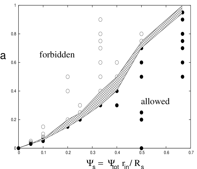
Figure 4: The 2-D parameter space $(a,\Psi_{s})$. Filled (black) circles correspond to the runs in which a stationary force-free solution has been obtained, while open (white) circles correspond to the runs that failed to converge to a stationary solution. The shaded band running diagonally across the plot represents the function $a_{\rm max}(R_{s})$, the maximal value of $a$ for which a force-free magnetic link can extend up to a given radial distance $R_{s}$ on the disk.

The single most important result of the present study is presented in Figure 4. This figure shows where in the two-dimensional $(a,\Psi_{s})$ parameter space force-free solutions exist and where they do not. Filled circles on this plot represent the runs in which convergence was achieved (allowed region), whereas open circles correspond to the runs that failed to converge to a suitable solution (forbidden region). The boundary $a_{\rm max}(\Psi_{s})$ between the allowed and forbidden regions is located somewhere inside the narrow hatched band that runs from the lower left to the upper right of the Figure [the finite width of the band represents the uncertainty in $a_{\rm max}(\Psi_{s})$ due to a limited number of runs]. As we can see, $a_{\rm max}(\Psi_{s})$ is a monotonically increasing function. In particular, in the limit $\Psi_{s}\rightarrow 0$, $a_{\rm max}$ indeed scales linearly with $\Psi_{s}$ and hence is inversely proportional to $R_{s}=r_{\rm in}\Psi_{\rm tot}/\Psi_{s}$, in full agreement with our expectations presented in § 3. However, this linear dependence no longer holds for finite values of $\Psi_{s}$ (and hence of $a_{\rm max}$).

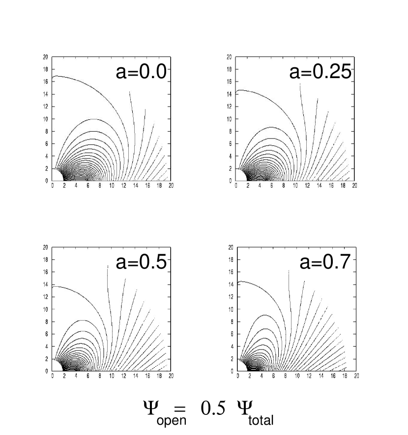
Figure 5: Contour plots of the magnetic flux function $\Psi(r,\theta)$ for four values of the black hole specific angular momentum: $a=0.0$, 0.25, 0.5, and 0.7; the amount of open poloidal flux in all cases is $\Psi_{s}=0.5\Psi_{\rm tot}$ (corresponding to $R_{s}=2r_{\rm in}$).

In order to study the effect that black hole spin has on the solutions, we concentrate on several values of $a$ for a fixed value of $\Psi_{s}$. In particular, we choose $\Psi_{s}=0.5$ [that corresponds to $R_{s}=2r_{\rm in}(a)$] and considered four values of‘$a$: $a=0$, $a=0.25$, $a=0.5$, and $a=0.7$. Thus, Figure 5 shows the contour plots of the poloidal magnetic flux for these four cases. We see that the flux surfaces inflate somewhat with increased $a$, but this expansion is not very dramatic, even in the case $a=0.7$, which is very close to the critical value $a_{\rm max}(\Psi_{s}=0.5)$ that corresponds to a sudden loss of equilibrium. We note that this finding is completely in line with our discussion in § 3.

The next three Figures present the plots of three important functions that characterize the solutions. In each Figure there are four curves corresponding to our selected values $a=0$, 0.25, 0.5, and 0.7 for $\Psi_{s}=0.5$. Figure 6 shows the event-horizon flux distribution $\Psi_{0}(\theta)$; Figure 7 shows the poloidal-current function $I(\Psi)$; and Figure 8 shows the position of the inner light cylinder described in terms of the lapse function $\alpha_{\rm LC}(\theta)$.

In Figure 6 we also plot $\Psi_{0}^{(0)}(\theta)$ corresponding to the simple split-monopole solution with uniform radial field at the horizon. Note that on the horizon we have $\Delta=0$ and hence $\Sigma=r_{H}^{2}+a^{2}=2Mr_{H}$; therefore

$$B_{\hat{r}}={1\over{\varpi\rho}}\Psi_{\theta}={1\over{\Sigma\sin\theta}}\Psi_{\theta}={1\over{2Mr_{H}}}\,{1\over{\sin\theta}}\,\Psi_{\theta}\,,\qquad r=r_{H}\,.$$ (51)

Thus, $B_{\hat{r}}(\theta)={\rm const}$ corresponds to $\Psi_{0}^{(0)}(\theta)=\Psi_{s}+(\Psi_{\rm tot}-\Psi_{s})(1-\cos\theta)$, independent of $a$. This function is plotted in Figure 6 (the dashed line) for comparison with the actual solutions. We see that the deviation from $\Psi_{0}^{(0)}(\theta)$ becomes noticeable only when $a$ approaches 1.

Figure 8 shows $\alpha_{\rm LC}(\theta)$. An interesting feature here is that the light cylinder reaches the event horizon at some intermediate angle $0<\theta_{\rm co}<\pi/2$ for small values of $a$. This is because, when $a<0.359..\,M$, the inner edge of a Keplerian disk rotates faster than the black hole; correspondingly, somewhere in the disk there exists a corotation point $r_{\rm co}>r_{\rm in}$ such that $\Omega_{K}(r_{\rm co})=\Omega_{H}$. The field line $\Psi_{\rm co}$ threading the disk at this point corotates with the black hole. Therefore, at the point $\theta_{\rm co}$ where this line intersects the horizon, we have $\delta\Omega=0$, and so this point ($r=r_{H},\theta=\theta_{\rm co}$) has to lie on the light cylinder. The location $\theta_{\rm co}$ of this point moves towards the equator when $a$ is increased and reaches it at $a=0.359..\,M$. For larger values of $a$, the entire disk outside of the ISCO rotates slower than the black hole and the light cylinder touches the horizon only at the pole $\theta=0$.

Finally, we also computed all the electric and magnetic field components and checked that $E^{2}<B^{2}$ everywhere outside the horizon.

5 Astrophysical Implications/Consequences

In this section we’ll discuss the exchange of energy and angular momentum between the black hole and the disk. Apart from the question of existence of solutions, this issue is one of the most important for actual astrophysical applications. Fortunately, once a particular solution describing the magnetosphere is obtained, computing the energy and angular momentum transported by the magnetic field becomes very simple.

Indeed, according to MT82, angular momentum and red-shifted energy (i.e., ”energy at infinity”) are transported along the poloidal field lines through the force-free magnetosphere without losses. Thus, the amount of angular momentum $\Delta L$ transported out in a unit of global time $t$ through a region between two neighboring poloidal flux surfaces, $\Psi$ and $\Psi+\Delta\Psi$, as given by equation (7.6) of MT82 (modified to suit our choice of notation), is

$${{d\Delta L}\over{dt}}=-{1\over 2}\,I\Delta\Psi\,,$$ (52)

and the red-shifted power—flux of redshifted energy per unit global time $t$— is expressed as

$$\Delta P=-{1\over 2}\,\Omega_{F}I\,\Delta\Psi\,,$$ (53)

(see eq. [7.8] of MT82).

Then, taking into account the contributions from both hemispheres and both sides of the disk, we can compute the total magnetic torque exerted by the hole onto the disk per unit $t$ as

$${{dL}\over{dt}}=-\int\limits_{\Psi_{s}}^{\Psi_{\rm tot}}I(\Psi)d\Psi\,,$$ (54)

and, correspondingly, the total red-shifted power transferred from the hole onto the disk via Poynting flux is

$$P=-\int\limits_{\Psi_{s}}^{\Psi_{\rm tot}}\Omega_{F}(\Psi)I(\Psi)d\Psi\,.$$ (55)

Next, since in our problem we have an explicit mapping (42) between $\Psi$ and the radial coordinate $r$ on the disk, we can immediately write down expressions for the radial distributions of angular momentum and red-shifted energy deposited on the disk per unit global time:

$${{d\Delta L(r)}\over{dt}}=-I[\Psi_{d}(r)]\,{{d\Psi_{d}}\over dr}\,dr\,,$$ (56)

and

$$\Delta P(r)=-\Omega_{K}(r)\,I[\Psi_{d}(r)]\,{{d\Psi_{d}}\over dr}\,dr\,.$$ (57)

Figures 9 and 10 show these distributions for our selected cases $a=0.25$, 0.5, and 0.7 for fixed $\Psi_{s}=0.5$. We see that in the case $a=0.25$ there is a corotation point $r_{\rm co}$ on the disk such that $\Omega_{\rm disk}>\Omega_{H}$ inside $r_{\rm co}$ and $\Omega_{\rm disk}<\Omega_{H}$ outside $r_{\rm co}$. Correspondingly, both angular memontum and red-shifted energy flow from the inner ($r<r_{\rm co}$) part of the disk to the black hole and from the hole to the outer ($r>r_{\rm co}$) part of the disk. At larger values of $a$, however, the Keplerian angular velocity at $r=r_{\rm in}$ is smaller than the black hole’s rotation rate and there is no corotation point; correspondingly, both angular momentum and redshifted energy flow from the hole to the disk. Also, as can be seen in Figures 9 and 10, the deposition of these quantities becomes strongly concentrated near the disk’s edge, especially at higher values of $a$.

Next, Figures 11 and 12 demonstrate the dependence of the total integrated angular momentum and red-shifted energy fluxes (54)–(55) on the black hole spin $a$ for a fixed value of $\Psi_{s}=0.5$. We see that both quantities are negative at small values of $a$ (meaning a transfer from the disk to the hole,) but then increase and become positive at larger $a$. The angular momentum transfer rate depends roughly linearly on $a$, whereas the red-shifted power $P(a)$ grows even faster, especially at large values of $a$. It is also interesting to note that the two quantities go through zero at slightly different values of the spin parameter: $dL/dt$ becomes zero at $a\approx 0.23$, while $P=0$ at $a\approx 0.26$. This means that it possible to have the total angular momentum flow from the hole to the disk and the total power flow from the disk to the hole at the same time.

6 Conclusions

In this paper we investigated the structure and the conditions for the existence of a force-free magnetosphere linking a rotating Kerr black hole to its accretion disk. We assumed that the magnetosphere is stationary, axisymmetric, and degenerate and that the disk is thin, ideally conducting, and Keplerian and that it is truncated at the Innermost Stable Circular Orbit. Our main goal was to determine under which conditions a force-free magnetic field can connect the hole directly to the disk and how the black hole rotation limits the radial extent of such a link on the disk surface.

We first introduced (in § 3) a very simple but robust physical argument that shows that, generally, magnetic field lines connecting the polar region of a spinning black hole to arbitrarily remote regions of the disk cannot be in a force-free equilibrium. The basic reason for this can be described as follows. Since the field lines threading the horizon have to first cross the inner light cylinder, and since they generally rotate at a rate that is different from the rotation rate of the black hole, these field lines have to be bent somewhat. In other words, they develop a toroidal magnetic field component, just like the open field lines crossing the outer light cylinder in a pulsar magnetosphere. In the language of the Membrane Paradigm (see Thorne et al. 1986), this toroidal field is needed so that the field lines could slip resistively across the stretched event horizon. The next step in our argument is to look at those field lines that connect the polar region of the horizon to the disk somewhere far away from the black hole. In a force-free magnetosphere, toroidal flux spreads along field lines to keep the poloidal current $I\sim B_{\hat{\phi}}\alpha\varpi$ constant along the field. Then one can show that the outward pressure of the toroidal field generated due to the black hole rotation turns out to be so large that it cannot be confined by the poloidal field tension at large enough distances. In other words, the field lines under consideration cannot be in a force-free equilibrium. Furthermore, one can generalize this argument to the case of closed magnetospheres of finite size and derive a conjecture that the maximal radial extent $R_{\rm max}$ of the magnetically-coupled region on the disk surface should scale inversely with the black hole spin parameter $a$ in the limit $a\rightarrow 0$.

In order to verify this hypothesis and to study the detailed structure of magnetically-coupled disk–hole configurations, we have obtained numerical solutions of the general-relativistic force-free Grad–Shafranov equation corresponding to partially-closed field configurations (shown in Fig. 3). This is an nonlinear 2nd-order partial differential equation for the poloidal flux function $\Psi(r,\theta)$ and it is the main equation governing the system’s behavior.

An additional complication in this problem arises from the need to specify two free functions that enter the force-free Grad–Shafranov equation; these are the field-line angular velocity $\Omega_{F}(\Psi)$ and the poloidal current $I(\Psi)$. Because all the field lines are assumed to be frozen into the disk, the first of this functions is determined in a fairly straightforward way. Namely, for any given field line $\Psi$, $\Omega_{F}(\Psi)$ is just the Keplerian angular velocity at this line’s footpoint on the disk. Specifying the poloidal current, on the other hand, is a much more difficult and nontrivial task. The reason for this is that it cannot be just prescribed explicitly on any given surface and one should look more thoroughly into the mathematical nature of the Grad–Shafranov equation itself to determine $I(\Psi)$. In particular, the most important feature of the Grad–Shafranov equation in this regard is that it becomes singular on two surfaces, the event horizon and the inner light cylinder. This observation is very useful because one can impose a physically-motivated regularity condition at each of these surfaces. One of the most important ideas in our analysis is that one can use the light-cylinder regularity condition to determine, using an iterative procedure, the poloidal current $I(\Psi)$, similar to the way it was done by CKF99 in the context of pulsar magnetospheres.

As for the singularity at the event horizon, it is also very important. Basically, it tells us that it is not possible to prescribe an arbitrary boundary condition at the horizon; instead, one can only impose a certain physical condition of regularity there. When combined with the Grad–Shafranov equation itself, this regularity requirement results in a single relationship (historically known as the horizon boundary condition, first derived by Znajek 1977) between three functions: the horizon flux distribution $\Psi_{0}(\theta)$, and the two free functions, $\Omega_{F}(\Psi)$ and $I(\Psi)$ (e.g., Beskin 1997; Beskin & Kuznetsova 2000). What’s important is that there are no other independent relationships that can be specified on this surface. In practical terms, this means that this condition should be used to determine the function $\Psi_{0}(\theta)$ in terms of $\Omega_{F}(\Psi)$ and $I(\Psi)$, which therefore must be determined outside the horizon. This fact helps to alleviate some of the causality issues raised by Punsly (1989, 2001, 2003) and by Punsly & Coroniti (1990).

Since one of the goals of this work was to study the dependence $R_{\rm max}(a)$, we performed a series of computations corresponding to various values of two parameters: the black hole spin parameter $a$ and the the magnetic link’s radial extent $R_{s}$ on the disk surface (the field lines anchored to the disk beyond $R_{s}$ were taken to be open and non-rotating). At the same time, the disk boundary conditions were kept the same in all these runs, namely, $\Psi_{d}(r)=\Psi_{\rm tot}r_{\rm in}(a)/r$. Therefore, varying the value of $R_{s}$ for fixed $a$ was equivalent to varying the amount $\Psi_{s}$ of open magnetic flux threading the disk.

Whereas for some pairs of values of $a$ and $\Psi_{s}$ we were able to achieve a convergent force-free solution, for others we were not. Thus, as one of the main results of our computations, we were able to chart out the allowed and the forbidden domains in the two-parameter space $(a,\Psi_{s})$. The boundary between these two domains is a curve $a_{\rm max}(\Psi_{s})$, which can be easily remapped into the curve $R_{\rm max}(a)$. As can be seen in Figure 4, this is a monotonically rising curve with the asymptotic behavior $a_{\rm max}\propto\Psi_{s}$ as $\Psi_{s}\rightarrow 0$, which is in line with our predictions.

We also computed the total angular momentum and red-shifted energy exchanged in a unit of global time $t$ between the hole and the disk through magnetic coupling. We studied the dependence of these quantities on the black hole spin parameter $a$ and found that the angular momentum transfer rate rises roughly linearly with $a$; it is negative for small $a$ (meaning the angular momentum transfer to the hole) and reverses sign around $a\approx 0.23$ (for $\Psi_{s}=0.5\Psi_{\rm tot}$). The total energy transfer increases with $a$ at an accelerated (i.e., faster than linear) rate, especially at larger values of $a$; it is also negative at small $a$, but becomes positive around $a=0.26$. This means that there is a narrow range $0.23..<a<0.26..$ where the integrated angular momentum flows from the hole to the disk, whereas the integrated red-shifted energy flows in the opposite direction.

Finally, we note that, in the case of open or partially-open field configuration responsible for the Blandford–Znajek process, one has to consider magnetic field lines that extend from the event horizon out to infinity. Since these field lines are not attached to a heavy infinitely conducting disk, their angular velocity $\Omega_{F}(\Psi)$ cannot be explicitly prescribed; it becomes just as undetermined as the poloidal current $I(\Psi)$ they carry. Fortunately, however, these field lines now have to cross two light cylinders (the inner one and the outer one). Since each of these is a singular surface of the Grad–Shafranov equation, one can impose corresponding regularity conditions on these two surfaces. Thus, we propose that one should be able to devise an iterative scheme that uses the two light-cylinder regularity conditions in a coordinated manner to determine the two free functions $\Omega(\Psi)$ and $I(\Psi)$ simultaneously, as a part of the overall solution process. At the same time, the regularity conditions at the event horizon and at infinity could be used to obtain the asymptotic poloidal flux distributions at $r=r_{H}$ and at $r\rightarrow\infty$, respectively. We realise of course that iterating with respect to two functions simultaneously may be a very difficult task. This purely technical obstacle (in addition to having to deal with the separatrix between the open- and closed-field regions) is the primary reason why, in this paper, we have restricted ourselves to a configuration which has no open field lines extending from the black hole to infinity. We leave this problem as a topic for future research.

It is possible that, instead of solving the Grad–Shafranov equation itself, the easiest and most practical way to achieve a stationary solution will be to use a time-dependent relativistic force-free code, such as one of those being developed now (Komissarov 2001, 2002a, 2004a; MacFadyen & Blandford 2003; Spitkovsky 2004; Krasnopolsky 2004, private communication).

I am very grateful to V. Beskin, O. Blaes, R.  Blandford, S. Boldyrev, A. Königl, B. C. Low, M. Lyutikov, A. MacFadyen, V. Pariev, B. Punsly, and A. Spitkovsky for many fruitful and stimulating discussions. I also would like to express my gratitude to the referee of this paper (Serguei Komissarov) for his very useful comments and suggestions that helped improve the paper. This research was supported by the National Science Foundation under Grant No. PHY99-07949.

7 References

Agol, E., & Krolik, J. H. 2000, ApJ, 528, 161

Begelman, M. C., Blandford, R. D., & Rees, M. J. 1984, Rev. Mod. Phys., 56, 255

Beskin, V. S., & Par’ev, V. I. 1993, Phys. Uspekhi, 36, 529

Beskin, V. S. 1997, Phys. Uspekhi, 40, 659

Beskin, V. S. 2003, Phys. Uspekhi, 46, 1209

Beskin, V. S., & Kuznetsova, I. V. 2000, Nuovo Cimento, 115, 795; preprint (astro-ph/0004021)

Blandford, R. D. 1976, MNRAS, 176, 465

Blandford, R. D. 1999, in Astrophysical Disks: An EC Summer School, ed. J. A. Sellwood & J. Goodman (San Francisco: ASP), ASP Conf. Ser. 160, 265; preprint (astro-ph/9902001)

Blandford, R. D. 2000, Phil. Trans. R. Soc. Lond. A, 358, 811; preprint (astro-ph/0001499)

Blandford, R. D. 2002, in ”Lighthouses of the Universe”, eds. Gilfanov, M. et al. (New York: Springer), 381

Blandford, R. D., & Znajek, R. L. 1977, MNRAS, 179, 433 (BZ77)

Blandford, R. D., & Payne, D. G. 1982, MNRAS, 199, 883

Contopoulos, I., Kazanas, D., & Fendt, C. 1999, ApJ, 511, 351

Damour, T. 1978, Phys. Rev. D, 18, 3589

Fendt, C. 1997, A&A, 319, 1025

Gammie, C. F. 1999, ApJ, 522, L57

Ghosh, P., & Abramowicz, M. A. 1997, MNRAS, 292, 887

Gruzinov, A. 1999, preprint (astro-ph/9908101)

Hawley, J. F., & Krolik, J. H. 2001, ApJ, 548, 348

Hirose, S., Krolik, J. H., de Villiers, J.-P., & Hawley, J. F. 2004, ApJ, 606, 1083

Hirotani, K., Takahashi, M., Nitta, S.-Y., & Tomimatsu, A. 1992, ApJ, 386, 455

Komissarov, S. S. 2001, MNRAS, 326, L41

Komissarov, S. S. 2002a, MNRAS, 336, 759

Komissarov, S. S. 2002b, preprint (astro-ph/0211141)

Komissarov, S. S. 2004a, MNRAS, 350, 427

Komissarov, S. S. 2004b, MNRAS, 350, 1431

Krolik, J. H. 1999a, ApJ, 515, L73

Krolik, J. H. 1999b, Active Galactic Nuclei: From The Central Black Hole To The Galactic Environment (Princeton: Princeton Univ. Press)

Levinson, A. 2004, ApJ, 608, 411

Li, L.-X. 2000, ApJ, 533, L115

Li, L.-X. 2001, in X-ray Emission from Accretion onto Black Holes, ed. T. Yaqoob & J. H. Krolik, JHU/LHEA Workshop, June 20-23, 2001

Li, L.-X. 2002a, ApJ, 567, 463

Li, L.-X. 2002b, A&A, 392, 469

Li, L.-X. 2004, preprint (astro-ph/0406353)

Livio, M., Ogilvie, G. I., & Pringle, J. E. 1999, ApJ, 512, 100

Lovelace, R. V. E. 1976, Nat., 262, 649

Macdonald, D., & Thorne, K. S. 1982, MNRAS, 198, 345 (MT82)

Macdonald, D. A. 1984, MNRAS, 211, 313

Macdonald, D. A., & Suen, W.-M. 1985, Phys. Rev. D, 32, 848

MacFadyen, A. I., & Blandford, R. D. 2003, AAS HEAD Meeting 35, 20.16

Nitta, S.-Y., Takahashi, M., & Tomimatsu, A. 1991, Phys. Rev. D, 44, 2295

Ogura, J., & Kojima, Y. 2003, Prog. Theor. Phys., 109, 619

Phinney, E. S. 1983, in Astrophysical Jets, ed. A. Ferrari & A. G.Pacholczyk (Dordrecht: Reidel), 201

Punsly, B. 1989, Phys. Rev. D, 40, 3834

Punsly, B. 2001, Black Hole Gravitohydromagnetics (Berlin: Springer)

Punsly, B. 2003, ApJ, 583, 842

Punsly, B. 2004, preprint (astro-ph/0407357)

Punsly, B., & Coroniti, F. V. 1990, ApJ, 350, 518

Spitkovsky, A. 2004, in IAU Symp. 218, Young Neutron Stars and Their Environment, ed. F. M. Camilo & B. M. Gaensler (San Francisco: ASP), 357; preprint (astro-ph/0310731)

Takahashi, M. 2002, ApJ, 570, 264

Thorne, K. S. 1974, ApJ, 191, 507

Thorne, K. S., Price, R. H., & Macdonald, D. A. 1986, Black Holes: The Membrane Paradigm (New Haven: Yale Univ. Press)

Uzdensky, D. A., Königl, A., & Litwin, C. 2002, ApJ, 565, 1191

Uzdensky, D. A., 2002a, ApJ, 572, 432

Uzdensky, D. A., 2002b, ApJ, 574, 1011

Uzdensky, D. A., 2003, ApJ, 598, 446

Uzdensky, D. A., 2004, ApJ, 603, 652

van Ballegooijen, A. A. 1994, Space Sci. Rev., 68, 299

van Putten, M. H. P. M. 1999, Science, 284, 115

van Putten, M. H. P. M., & Levinson, A. 2003, ApJ, 584, 937

Wang, D. X., Xiao, K., & Lei, W. H. 2002, MNRAS, 335, 655

Wang, D.-X., Lei, W. H., & Ma, R.-Y. 2003a, MNRAS, 342, 851

Wang, D.-X., Ma, R.-Y., Lei, W.-H., & Yao, G.-Z. 2003b, ApJ, 595, 109

Wang, D.-X., Ma, R.-Y., Lei, W.-H., & Yao, G.-Z. 2004, ApJ, 601, 1031

Znajek, R. L. 1977, MNRAS, 179, 457

Znajek, R. L. 1978, MNRAS, 185, 833

Figure 1: Schematic drawing of an open black hole – disk magnetosphere, commonly associated with the Blandford–Znajek (BZ77) process. Rotational energy and angular momentum are extracted from both the black hole and the disk and are transported away by the magnetic field.

Figure 2: Schematic drawing of a fully-closed black hole – disk magnetosphere. Energy and angular momentum are exchanged between the hole and the disk through a direct magnetic link.

Figure 3: Schematic drawing of a black hole – disk magnetosphere with a radially-limited magnetic connection. Here, only the inner part of the disk is coupled magnetically to the hole (closed field region), whereas the field lines attached to the outer part of the disk are open and extend to infinity.

Figure 6: The horizon poloidal flux distribution $\Psi_{0}(\theta)$ for several values of $a$ and a single value $\Psi_{s}=0.5\Psi_{\rm tot}$ of the open magnetic flux (corresponding to $R_{s}=2\,r_{\rm in}(a)$.

Figure 7: Poloidal current $I$ as a function of poloidal magnetic flux $\Psi$ for several values of $a$ and a single value $\Psi_{s}=0.5\Psi_{\rm tot}$.

Figure 8: The position of the inner light cylinder represented by the lapse function $\alpha_{\rm LC}(\theta)$ for several values of $a$. The light cylinder touches the horizon at the pole $\theta=0$ and, for $a<0.36$, at the point $\theta=\theta_{\rm co}$ where the corotation field line $\Psi_{\rm co}\equiv\Psi_{d}(r_{\rm co})$ intersects the horizon.

Figure 9: Radial distribution $d^{2}L/drdt$ of the magnetic torque per unit radius $r$ on the disk surface for $a=0.25$, 0.5, and 0.7.

Figure 10: Radial distribution $dP/dr$ of the red-shifted power per unit radius $r$ on the disk surface for $a=0.25$, 0.5, and 0.7.

Figure 11: The dependence of the total magnetic torque between the black hole and the disk on the hole’s spin parameter $a$ for fixed $R_{s}=2r_{\rm in}$.

Figure 12: The dependence of the total red-shifted power exchanged magnetically between the black hole and the disk on the hole’s spin parameter $a$ for fixed $R_{s}=2r_{\rm in}$.