A Running Spectral Index in Supersymmetric Dark-Matter
Models with Quasi-Stable Charged Particles

Abstract

We show that charged-particles decaying in the early Universe can induce a scale-dependent or ‘running’ spectral index in the small-scale linear and nonlinear matter power spectrum and discuss examples of this effect in minimal supersymmetric models in which the lightest neutralino is a viable cold-dark-matter candidate. We find configurations in which the neutralino relic density is set by coannihilations with a long-lived stau, and the late decay of staus partially suppresses the linear matter power spectrum. Nonlinear evolution on small scales then causes the modified linear power spectrum to evolve to a nonlinear power spectrum similar (but different in detail) to models parametrized by a constant running $\alpha_{s}=dn_{s}/d{\rm ln}k$ by redshifts of 2 to 4. Thus, Lyman-$\alpha$ forest observations, which probe the matter power spectrum at these redshifts, might not discriminate between the two effects. However, a measurement of the angular power spectrum of primordial 21-cm radiation from redshift $z\approx 30$–$200$ might distinguish between this charged-decay model and a primordial running spectral index. The direct production of a long-lived charged particle at future colliders is a dramatic prediction of this model.

I Introduction

While recent cosmological observations provide convincing evidence that nonbaryonic dark matter exists CMBconstraints , we do not know the detailed particle properties of the dark matter, nor the particle spectrum of the dark sector. There has been considerable phenomenological effort towards placing model-independent limits on the possible interactions of the lightest dark-matter particle (LDP) in an attempt to try and identify candidates within detailed particle theories or rule out particular candidate theories. For instance, models with stable charged dark matter have been ruled out Gould:1989gw , while significant constraints have been made to dark-matter models with strong interactions Starkman:1990nj , self-interactions Carlson:1992 ; Spergel:1999mh , and a millicharge Davidson:2000hf ; Dubovsky:2003yn . Recently, it was shown that a neutral dark-matter particle with a relatively large electric or magnetic dipole moment remains a phenomenologically viable candidate Sigurdson:2004zp .

Concurrent with this phenomenological effort, theorists have taken to considering physics beyond the standard model in search of a consistent framework for viable dark-matter candidates. The leading candidates, those that produce the correct relic abundance and appear in minimal extensions of the standard model (often for independent reasons), are the axion axionreviews and weakly interacting massive particles (WIMPs), such as the neutralino, the lightest mass eigenstate from the superposition of the supersymmetric partners of the $U(1)$ and $SU(2)$ neutral gauge bosons and of the neutral Higgs bosons Jungman:1995df ; larsrev . However, other viable candidates have also been considered recently, such as gravitinos or Kaluza-Klein gravitons produced through the late decay of WIMPs Feng:2003xh ; Feng:2004zu . These latter candidates are an interesting possibility because the constraints to the interactions of the LDP do not apply to the next-to-lightest dark-matter particle (NLDP), and the decay of the NLDP to the LDP at early times may produce interesting cosmological effects; for instance, the reprocessing of the light-element abundances formed during big-bang nucleosynthesis Feng:2003uy ; karsten , or if the NLDP is charged, the suppression of the matter power spectrum on small scales and thus a reduction in the expected number of dwarf galaxies Sigurdson:2003vy .

In this paper we describe another effect charged NLDPs could have on the matter power spectrum. If all of the present-day dark matter is produced through the late decay of charged NLDPs, then, as discussed in Ref. Sigurdson:2003vy , the effect is to essentially cut off the matter power spectrum on scales that enter the horizon before the NLDP decays. However, if only a fraction $f_{\phi}$ of the present-day dark matter is produced through the late decay of charged NLDPs, the matter power spectrum is suppressed on small scales only by a factor $(1-f_{\phi})^{2}$. This induces a scale-dependent spectral index for wavenumbers that enter the horizon when the age of the Universe is equal to the lifetime of the charged particles. What we show below is that, for certain combinations of $f_{\phi}$ and of the lifetime of the charged particle $\tau$, this suppression modifies the nonlinear power spectrum in a way similar (but different in detail) to the effect of a constant $\alpha_{s}\equiv dn_{s}/d{\rm ln}k\neq 0$. Although these effects are different, constraints based on observations that probe the nonlinear power spectrum at redshifts of 2 to 4, such as measurements of the Lyman-$\alpha$ forest, might confuse a running index with the effect we describe here even if parametrized in terms of a constant $\alpha_{s}$. This has significant implications for the interpretation of the detection of a large running of the spectral index as a constraint on simple single-field inflationary models. The detection of a unexpectedly large spectral running in future observations could instead be revealing properties of the dark-matter particle spectrum in conjunction with a more conventional model of inflation. We note that the Sloan Digital Sky Survey Lyman-$\alpha$ data Seljak:2004xh has significantly improved the limits to constant-$\alpha_{s}$ models compared to previous measurements alone CMBconstraints ; Seljak:2003jg ; Tegmark:2003ud . A detailed study of the ($\tau$,$f_{\phi}$) parameter space using these and other cosmological data would also provide interesting limits to the models we discuss here.

While, even with future Lyman-$\alpha$ data, it may be difficult to discriminate the effect of a constant running of the spectral index from a scale-dependent spectral index due to a charged NLDP, other observations may nevertheless discriminate between the two scenarios. Future measurements of the power spectrum of neutral hydrogen through the 21cm-line might probe the linear matter power spectrum in exquisite detail over the redshift range $z\approx 30-200$ at comoving scales less than 1 Mpc and perhaps as small as $0.01$ Mpc Loeb:2003ya ; such a measurement could distinguish between the charged-particle decay scenario we describe here and other modifications to the primoridal power spectrum. If, as in some models we discuss below, the mass of these particles is in reach of future particle colliders the signature of this scenario would be spectacular and unmistakable—the production of very long-lived charged particles that slowly decay to stable dark matter.

Although we describe the cosmological side of our calculations in a model-independent manner, remarkably, there are configurations in the minimal supersymmetric extension of the standard model (MSSM) with the right properties for the effect we discuss here. In particular, we find that if the LSP is a neutralino quasi-degenerate in mass with the lightest stau, we can naturally obtain, at the same time, LDPs providing the correct dark matter abundance $\Omega_{\chi}h^{2}=0.113$ CMBconstraints and NLDPs with the long lifetimes and the sizable densities in the early Universe needed in the proposed scenario. Such configurations arise even in minimal supersymmetric schemes, such as the minimal supergravity (mSUGRA) scenario msugra and the minimal anomaly-mediated supersymmetry-breaking (mAMSB) model mamsb . This implies that a detailed study of the ($\tau$,$f_{\phi}$) parameter space using current and future cosmological data may constrain regions of the MSSM parameter space that are otherwise viable. Furthermore, we are able to make quantitative statements about testing the scenario we propose in future particle colliders or dark matter detection experiments.

The paper is organized as follows: We first review in Section II how the standard calculation of linear perturbations in an expanding universe must be modified to account for the effects of a decaying charged species, calculate the linear matter power spectrum and discuss the constraints to this model from big bang nucleosynthesis (BBN) and the spectrum of the cosmic microwave background (CMB). In Section III we briefly discuss how we estimate the nonlinear power spectrum from the linear power spectrum and present several examples. In Section IV we discuss how measurements of the angular power spectra of the primordial 21-cm radiation can be used to distinguish this effect from other modifications to the primordial power spectrum. In Section V we describe how this scenario can be embedded in a particle physics model, concluding that the most appealing scheme is one where long lifetimes are obtained by considering nearly degenerate LDP and NLDP masses. In Section VI we compute the lifetimes of charged next-to-lightest supersymmetric particles (NLSPs) decaying into neutralino LSPs, and show that, in the MSSM, the role of a NLDP with a long lifetime can be played by a stau only. In Section VII we estimate what fraction of charged to neutral dark matter is expected in this case, while in Section VIII we describe how consistent realizations of this scenario can be found within the parameter space of mSUGRA and mAMSB. Finally, in Section IX we discuss the expected signatures of this scenario at future particle colliders, such as the large hadron collider (LHC), and prospects for detection in experiments searching for WIMP dark matter. We conclude with a brief summary of our results in Section X.

II Charged-Particle Decay

In this section we discuss how the decay of a charged particle $\phi$ (the NLDP) to a neutral particle $\chi$ (the LDP) results in the suppression of the linear matter power spectrum on small scales.

As the $\phi$ particles decay to $\chi$ particles, their comoving energy density decays exponentially as

$$\rho_{\phi}a^{3}=m_{\phi}n_{\phi_{0}}e^{-t/\tau}\,,$$ (1)

increasing the comoving energy density of $\chi$ particles as

$$\rho_{\chi}a^{3}=m_{\chi}n_{\chi_{0}}(1-f_{\phi}e^{-t/\tau})\,.$$ (2)

Here $n_{\chi_{0}}=\Omega_{\chi}\rho_{crit}/m_{\chi}$ is the comoving number density of dark matter, and $n_{\phi_{0}}=f_{\phi}n_{\chi_{0}}$ is the comoving number density of dark matter produced through the decay of $\phi$ particles, $a$ is the scale factor, and $t$ is the cosmic time.

Since the $\phi$ particles are charged, they are tightly coupled to the ordinary baryons (the protons, helium nuclei, and electrons) through Coulomb scattering. It is therefore possible describe the combined $\phi$ and baryon fluids as a generalized baryon-like component $\beta$ as far as perturbation dynamics is concerned. We thus denote by $\rho_{\beta}=\rho_{b}+\rho_{\phi}$ the total charged-particle energy density at any given time. At late times, after nearly all $\phi$ particles have decayed, $\rho_{\beta}\simeq\rho_{b}$.

The relevant species whose perturbation dynamics are modified from the standard case are the stable dark matter (subscript $\chi$), the charged species (subscript $\beta$), and the photons (subscript $\gamma$). By imposing covariant conservation of the total stress-energy tensor, accounting for the Compton scattering between the electrons and the photons, and linearizing about a Friedmann-Robertson-Walker (FRW) Universe we arrive at the equations describing the evolution of linear fluid perturbations of these components in an expanding Universe.

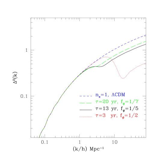
Figure 1: Shown is $\Delta^{2}(k)=k^{3}P(k)/2\pi^{2}$, the dimensionless matter power spectrum per logarithmic interval for the canonical $n_{s}=1$ $\Lambda$CDM model (dashed), for a model with $\tau=20~{}{\rm yr}$ and $f_{\phi}=1/7$ (long-dashed), for a model with $\tau=13~{}{\rm yr}$ and $f_{\phi}=1/5$ (solid), and for a model with $\tau=3~{}{\rm yr}$ and $f_{\phi}=1/2$ (dotted). Modes that enter the horizon be before the $\phi$ particles decay are suppressed by a factor of $(1-f_{\phi})^{2}$.

In the synchronous gauge, for the ‘$\beta$’ component, the perturbation evolution equations are

$$\dot{\delta}_{\beta}=-\theta_{\beta}-\frac{1}{2}\dot{h}\,,$$ (3)

and

$$\dot{\theta}_{\beta}=-\frac{\dot{a}}{a}\theta_{\beta} +c_{s}^{2}k^{2}\delta_{\beta}+\frac{4\rho_{\gamma}}{3\rho_{\beta}}an_{e}\sigma_{T}(\theta_{\gamma}-\theta_{\beta})\,.$$ (4)

Here and in what follows, $\delta_{X}={\delta\rho}_{X}/\rho_{X}$ is the fractional overdensity and $\theta_{X}=ikV_{X}$ is the divergence of the bulk velocity in Fourier space of a given species $X$. An overdot represents a derivative with respect to the conformal time. The number density of electrons is $n_{e}$, while $\sigma_{T}$ is the Thomson cross section. Because the $\phi$ particles and the baryons share a common bulk velocity and overdensity, these equations are identical to the standard perturbation equations for the baryons with the replacement $b\rightarrow\beta$ (see, for example, Ref. Ma:1995ey ). For the dark matter we find that

$$\dot{\delta}_{\chi}=-\theta_{\chi}-\frac{1}{2}\dot{h}+\lambda_{m}\frac{\rho_{\phi}}{\rho_{\chi}}\frac{a}{\tau}(\delta_{\beta}-\delta_{\chi})\,,$$ (5)

and

$$\dot{\theta}_{\chi}=-\frac{\dot{a}}{a}\theta_{\chi}+\lambda_{m}\frac{\rho_{\phi}}{\rho_{\chi}}\frac{a}{\tau}(\theta_{\beta}-\theta_{\chi})\,,$$ (6)

where $\lambda_{m}\equiv m_{\chi}/m_{\phi}=(1+\Delta m/m_{\chi})^{-1}$. The modifications to the photon perturbation evolution are negligibly small because $\phi$ decays during the radiation-dominated epoch when $\rho_{\phi}\ll\rho_{\gamma}$ and, as discussed below, for viable models $\lambda_{m}\simeq 1$ to prevent unreasonably large spectral distortions to the CMB.

Combining these equations with the (unmodified) equations for the neutrino perturbations we can solve for the linear power spectrum of matter fluctuations in this model. We have solved these equations using a modified version of cmbfast Seljak:1996is . In Fig. 1 we show the linear matter power spectrum in this model for several values of the $\phi$ lifetime $\tau$ and fraction $f_{\phi}$. As shown in this Figure, the small-scale density modes that enter the horizon before the $\phi$ particles decay (when the age of the Universe is less than $\tau$) are suppressed relative to the standard case by a factor of $(1-f_{\phi})^{2}$.

Since the decaying particles are charged, the production of the LDP will always be accompanied by an electromagnetic cascade. The latter could in principle reprocess the light elements produced during BBN, or induce unreasonably large spectral distortions to the CMB. We show here that in fact these effects are small for the models discussed in this paper.

The energy density released by the decay of $\phi$ particles can be parametrized as

$$\zeta_{EM}=\varepsilon_{EM}f_{\phi}Y_{\chi}\,,$$ (7)

where $\varepsilon_{EM}$ is the average electromagnetic energy released in a $\phi$ decay and $Y_{\chi}\equiv n_{\chi}/n_{\gamma}$ is the dark-matter to photon ratio. In the specific models we discuss below, $\varepsilon_{EM}\approx\Delta m/3$, and

$$Y_{\chi}=\frac{\Omega_{\chi}\rho_{c}}{m_{\chi}n_{\gamma}}=3\times 10^{-12}\left(\frac{{\rm TeV}}{m_{\chi}}\right)\left(\frac{\Omega_{\chi}}{0.23}\right)\,.$$ (8)

This yields

$$\zeta_{EM}\approx f_{\phi}\frac{\Delta m}{m_{\chi}}\left(\frac{\Omega_{\chi}}{0.23}\right)~{}{\rm eV}\,.$$ (9)

In the models we discuss below, $\Delta m/m_{\chi}\sim 10^{-4}$, and $f_{\phi}\leq 1/2$, giving $\zeta_{EM}\lesssim 5\times 10^{-5}$ eV. The limit derived from too much reprocessing of the BBN light element abundances is $\zeta_{EM}\lesssim 3.8~{}\tau_{\rm yr}^{1/4}\times 10^{-3}$ eV Cyburt:2002uv ; jedamzik where $\tau_{\rm yr}=\tau/(1~{}{{\rm yr}})$, so we are safely below this bound.

For $\tau_{\rm yr}\lesssim 300$, electromagnetic energy injection will result in a chemical-potential distortion to the CMB of Hu:1993gc

$$\mu=4.5~{}\tau_{\rm yr}^{1/2}\times 10^{-3}\left(\frac{\zeta_{EM}}{\rm eV}\right)e^{-0.128\tau_{\rm yr}^{-5/4}}\,$$ (10)

and so we expect $\mu\lesssim 2.0\times 10^{-7}$ — $2.3\times 10^{-6}$ for lifetimes between $\tau_{\rm yr}=1$ — $100$, below the current limit of $\mu<9\times 10^{-5}$ Fixsen:1996nj .

III The Nonlinear Power Spectrum

As density perturbations grow under the influence of gravity, linear evolution ceases to describe their growth and nonlinear effects must be taken into account. On large scales, where density perturbations have had insufficient time to become nonlinear, the linear matter power spectrum describes the statistics of density fluctuations. However, on small scales the full nonlinear matter power spectrum is required.

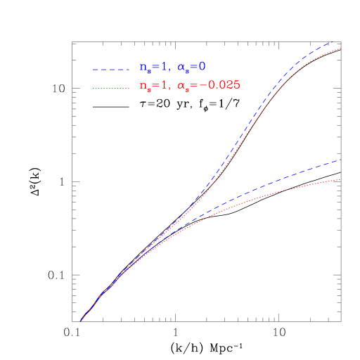
Figure 2: Shown at a redshift $z=4$ are $\Delta^{2}(k)=k^{3}P(k)/2\pi^{2}$, the nonlinear (upper curves) and linear (lower curves) dimensionless matter power spectra per logarithmic interval for the canonical $n_{s}=1$ $\Lambda$CDM model (dashed), for an $n_{s}=1$ model with $\tau=20~{}{\rm yr}$ and $f_{\phi}=1/7$ (solid), and for a running-index model with $n_{s}=1.00$ and $\alpha_{s}=-0.025$ (dotted). Although the linear power spectra differ significantly in these latter two models, nonlinear evolution causes them to have nearly degenerate nonlinear power spectra for $k/h\gtrsim 1.5~{}{\rm Mpc}^{-1}$.

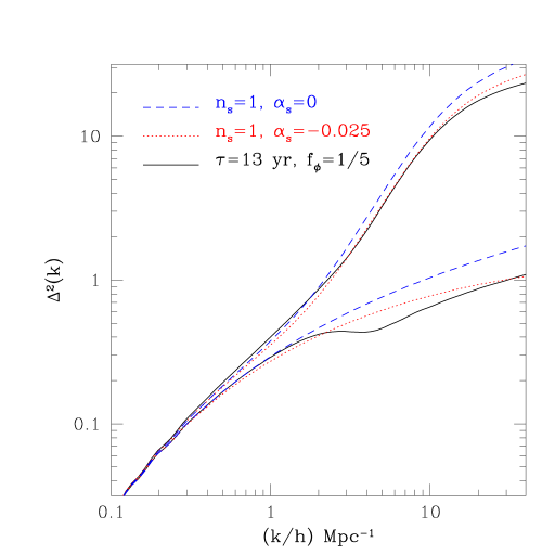
Figure 3: Shown at a redshift $z=4$ are $\Delta^{2}(k)=k^{3}P(k)/2\pi^{2}$, the nonlinear (upper curves) and linear (lower curves) dimensionless matter power spectra per logarithmic interval for the canonical $n_{s}=1$ $\Lambda$CDM model (dashed), for an $n_{s}=1$ model with $\tau=13~{}{\rm yr}$ and $f_{\phi}=1/5$ (solid), and for a running-index model with $n_{s}=1.00$ and $\alpha_{s}=-0.025$ (dotted). Nonlinear evolution causes these two models to have overlapping nonlinear power spectra for $2~{}{\rm Mpc}^{-1}\lesssim k/h\lesssim 10~{}{\rm Mpc}^{-1}$.

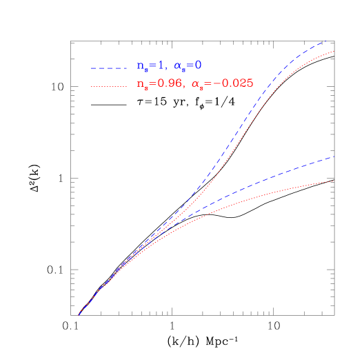
Figure 4: Shown at a redshift $z=4$ are $\Delta^{2}(k)=k^{3}P(k)/2\pi^{2}$, the nonlinear (upper curves) and linear (lower curves) dimensionless matter power spectra per logarithmic interval for the canonical $n_{s}=1$ $\Lambda$CDM model (dashed), for an $n_{s}=1$ model with $\tau=15~{}{\rm yr}$ and $f_{\phi}=1/4$ (solid), and for a running-index model with $n_{s}=0.96$ and $\alpha_{s}=-0.025$ (dotted). Nonlinear evolution causes the charged-decay model to match the canonical $\Lambda$CDM model for $k/h\lesssim 1.5~{}{\rm Mpc}^{-1}$ and the running-index model for $k/h\gtrsim 1.5~{}{\rm Mpc}^{-1}$.

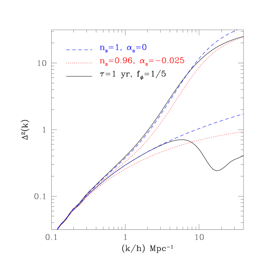
Figure 5: Shown at a redshift $z=4$ are $\Delta^{2}(k)=k^{3}P(k)/2\pi^{2}$, the nonlinear (upper curves) and linear (lower curves) dimensionless matter power spectra per logarithmic interval for the canonical $n_{s}=1$ $\Lambda$CDM model (dashed), for an $n_{s}=1$ model with $\tau=1~{}{\rm yr}$ and $f_{\phi}=1/2$ (solid), and for a running-index model with $n_{s}=0.96$ and $\alpha_{s}=-0.025$ (dotted). Despite the drastic change in the linear power spectrum nonlinear evolution causes the charged-decay model to match the canonical $\Lambda$CDM model for $k/h\lesssim 8~{}{\rm Mpc}^{-1}$ and the running-index model for $k/h\gtrsim 8~{}{\rm Mpc}^{-1}$.

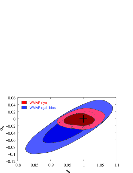
Figure 6: We reproduce here (with permission) Fig. 3 from Ref. Seljak:2004xh which illustrates the current constraints on the parameter $\alpha_{s}$. The charged-decay models produce changes to the nonlinear power spectrum similar to constant $\alpha_{s}\neq 0$ models within the WMAP+Lya contour shown here and the examples we show in Figs. 2–5 are denoted by the black circles (ours). However, the charged-decay models leave the CMB angular power spectra unaltered (corresponding to models with $\alpha_{s}=0$ on a line passing through the black cross). Matching to allowed constant-$\alpha_{s}$ models is conservative in this respect, and we thus expect the charged-decay models we have discussed in Figs. 2–5 to be consistent with current data.

In order to calculate the nonlinear power spectrum for a given model we have used the recently devised halofit method Smith:2002dz . This method uses higher-order perturbation theory in conjunction with the halo model of large-scale structure to determine the nonlinear power spectrum given a linear power spectrum. It has been shown to accurately reproduce the nonlinear power spectra of standard N-body simulations and, unlike the earlier mappings such as the Peacock and Dodds formula Peacock:1996ci , it is applicable in cases (like we consider here) when $\Delta^{2}(k)=k^{3}P(k)/2\pi^{2}$ is not a monotonic function. In particular we have checked that it approximately reproduces the shapes of the nonlinear power spectra determined in Ref. White:2000sy through N-body simulations in models where the linear power spectrum is completely cut off on small scales. As we are discussing here less drastic alterations to the linear power spectrum, we believe the halofit procedure provides an estimate of the nonlinear power spectrum adequate for illustrating the effect we describe in this paper. Any detailed study would require a full N-body simulation.

In Figs. 2–5 we show both the linear and nonlinear matter power spectra at redshift $z=4$ (data from measurements the Lyman-$\alpha$ forest probe redshifts 2–4 at wavenumbers $k/h\sim 0.1$–$10~{}{\rm Mpc}^{-1}$) for a charged-decay model, and for a model with a running spectral index. Although these models have different linear power spectra, nonlinear gravitational evolution causes these models to have nearly identical nonlinear power spectra over interesting ranges of wavenumbers. The lifetimes shown were chosen because they produce effects on scales that can be probed by measurements of the Lyman-$\alpha$ forest, while the values $f_{\phi}=(1/2,1/4,1/5,1/7)$ were chosen because they arise in the supersymmetric models we discuss below.

In Fig. 6 we show the current constraints on the ($n_{s}$,$\alpha_{s}$) parameter space from WMAP and SDSS Lyman-$\alpha$ forest data. The constant-$\alpha_{s}$ models we have compared our charged-decay model to lie within the WMAP+lya contours shown in the Figure. Since, in each case, the charged-decay model tends to interpolate between the standard $\Lambda$CDM model on larger scales (in particular on the scales probed by the CMB) and a constant-$\alpha_{s}$ running-index model on smaller scales, and both of them are allowed by these data, we expect the charged-decay models we have considered in Figs. 2–5 to be consistent with current data as well. We leave for future work the task of using a combined analysis of Lyman-$\alpha$ forest and other cosmological measurements to put limits directly on the ($f_{\phi}$,$\tau$) parameter space (and thus on the parameter space of the MSSM models we discuss below).

IV The 21 cm Power Spectrum

After recombination and the formation of neutral hydrogen, the gas in the Universe cools with respect to the CMB temperature $T_{\rm CMB}$ starting at at a redshift $z\sim 200$. The spin temperature $T_{s}$ of the gas, which measures the relative populations of the hyperfine levels of the ground state of hydrogen separated by the 21-cm spin-flip transition, remains collisionally coupled to the temperature $T_{b}$ of the baryons until a redshift $z\sim 30$ when collisions become inefficient and the spin temperature rises to $T_{\rm CMB}$. There is thus a window between $z\sim 30$–$200$ in which neutral hydrogen absorbs the CMB at a wavelength of $21~{}{\rm cm}$. It has recently been suggested that the angular fluctuations in the brightness temperature of the 21-cm transition within this window may be measured with future observations and used to constrain the matter power spectrum at these very high redshifts Loeb:2003ya .

At redshifts $z\gtrsim 30$, the matter power spectrum on the scales $k/h\sim 1-100~{}{\rm Mpc}^{-1}$ of interest here are still in the linear regime. As discussed in Ref. Loeb:2003ya , due to the unprecedented wealth of potential information contained in these $21$-cm measurements, models with a running index or other small-scale modifications of the matter power spectrum can in principle be distinguished from each other. Even if the charged-particle lifetime is so small that no significant modifications to the power spectrum occur on scales probed by other cosmological observations (like the model shown in Fig. 5), 21-cm observations might detect or constrain such effects on the linear matter power spectrum.

V The long lived charged next-to-lightest dark-matter particle

From the particle-physics point of view, the setup we have introduced may seem ad hoc. We need a pair of particles that share a conserved quantum number and such that the lightest, the LDP, is neutral and stable, while the other, the NLDP, is coupled to the photon and quasi-stable, in order to significantly contribute to the cosmological energy density at an intermediate stage in the structure-formation process. Such a picture requires three ingredients: (i) the relic abundance of the LDP must be compatible with the CDM component; (ii) the abundance of the NLDP must be at the correct level (namely, $\sim 1/5$ the total dark-matter density); and (iii) the NLDP must have the proper lifetime (i.e., $\tau\sim 10$ yr).

Let us start with the last requirement. One way to get the required lifetime is to introduce a framework with strongly-suppressed couplings. One such possibility is, for instance, to assume that the LDP is a stable super-weakly–interacting dark-matter particle, such as a gravitino LSP in R-parity–conserving supersymmetric theories or the Kaluza-Klein first excitation $G^{1}$ of the graviton in the universal extra-dimension scenario Servant:2002aq . The NLDP can have non-zero electric charge, but at the same time a super-weak decay rate into the LDP (with the latter being the only allowed decay mode). In models of gauge-mediated supersymmetry breaking, this might indeed be the case with a stau NLSP decaying into a gravitino LSP. In this specific example, we have checked that, to retrieve the very long lifetimes we introduced in our discussion, we would need to impose a small mass splitting between the NLSP and LSP, as well as to raise the mass scale of the LSP up to about 100 TeV. This value is most often considered uncomfortably large for a SUSY setup, and it also makes thermal production of LDPs or NLDPs unlikely, being near a scale at which the unitary bound Griest:1989wd gets violated. Without thermal production one would need to invoke first a mechanism to wipe out the thermal components and then provide a viable non-thermal production scheme that fixes the right portion of LDPs versus NLDPs. Finally, such heavy and extremely weakly-interacting objects would evade any dark-matter detection experiment, and would certainly not be produced at the forthcoming CERN Large Hadron Collider (LHC). This would then be a scheme that satisfies the three ingredients mentioned above, but that cannot be tested in any other way apart from cosmological observations.

An alternative (and to us, more appealing) scenario is one where long lifetimes are obtained by considering nearly degenerate LDP and NLDP masses. In this case, decay rates become small, without suppressed couplings, simply because the phase space allowed in the decay process gets sharply reduced. Sizeable couplings imply that, in the early Universe, the LDP and NLDP efficiently transform into each other through scattering from background particles. The small mass splitting, in turn, guarantees that the thermal-equilibrium number densities of the two species are comparable. To describe the process of decoupling and find the thermal relic abundance of these species, the number densities of the two have to be traced simultaneously, with the NLDP, being charged, playing the major role. This phenomenon is usually dubbed as coannihilation Griest:1990kh and has been studied at length, being ubiquitous in many frameworks embedding thermal-relic candidates for dark matter, including common SUSY schemes.

We will show below that sufficiently long lifetimes may be indeed obtained in the minimal supersymmetric standard model (MSSM), when the role of the NLDP is played by a stau nearly degenerate in mass with the lightest neutralino (with the former being the stable LSP and the thermal-relic CDM candidate we will focus on in the remainder of our discussion). A setup of this kind appears naturally, e.g., in minimal supergravity (mSUGRA) Ellis:2003cw . This is the SUSY framework with the smallest possible parameter space, defined by only four continuous entries plus one sign, and hence also one of the most severely constrained by the requirement that the neutralino relic density matches the value from cosmological observations. Neutralino-stau coannihilations determine one of the allowed regions, on the border with the region where the stau, which in the mSUGRA scheme is most often the lightest scalar SUSY particle, becomes lighter than the neutralino. Although a stau-neutralino mass degeneracy is not “generic” in such models, this scenario is economical in that the requirements of a long NLDP lifetime and of comparable LDP and NLDP relic abundances are both consequences of the mass degeneracy. In this sense, evidence for a running spectral index or any of the other observational features we discuss would simply help us sort out which configuration (if any) Nature has chosen for SUSY dark matter.

VI Lifetimes of charged NLSPs in the MSSM

We refer to a MSSM setup in which the lightest neutralino $\chi^{0}_{1}$ is the lightest SUSY particle. The charged particles that could play the role of the NLDP include: (1) scalar quarks, (2) scalar charged leptons, and (3) charginos. We now discriminate among these cases by the number of particles in the final states for the decay of NLSPs to neutralino LSPs.

Scalar quarks and leptons have as their dominant decay mode a prompt two-body final state; i.e., $\tilde{S}\rightarrow\chi^{0}_{1}S$, where we have labeled $\tilde{S}$ the SUSY scalar partner of the standard-model fermion $S$. A typical decay width for this process is $\mathcal{O}$(1) GeV, corresponding to a lifetime $\mathcal{O}$$(10^{-24})$ s. This holds whenever this final state is kinematically allowed; i.e., if $m_{\tilde{S}}>m_{S}+m_{\chi^{0}_{1}}$. If it is kinematically forbidden, there are two possibilities: squarks may either decay through CKM-suppressed flavor-changing processes or through four-body decays. For instance, the stop decay may proceed through $\tilde{t}\rightarrow\chi^{0}_{1}c$ or $\tilde{t}\rightarrow\chi^{0}_{1}bf\bar{f}^{\prime}$. On the other hand, within the same minimal–flavor-violation framework, scalar leptons are not allowed to decay in flavor-changing two-body final states, and only the four-body decay option remains.

The case for the chargino is different because this NLSP decay has a three-body final state, either with two quarks bound in a meson state — i.e., $\chi^{+}_{1}\rightarrow\chi^{0}_{1}\pi^{+}$ — or with a leptonic three body channel — i.e., $\chi^{+}_{1}\rightarrow\chi^{0}_{1}l^{+}\nu_{l}$. The latter final state becomes dominant, in particular, for electron-type leptons, $l=e$, if the mass splitting between NLSP and LSP becomes small.

We have listed all decay topologies as these are especially relevant when discussing the limit in which we force a reduction of the allowed decay phase-space volume; i.e., the limit in which the NLSP and LSP are quasi-degenerate in mass. Here we can also safely assume that the masses of the final-state particles, apart from the neutralino, are much smaller than the mass of the decaying particle. We can then consider the limit of a particle of mass $m_{\chi^{0}_{1}}+\Delta m$ decaying into a $\chi^{0}_{1}$ and $n-1$ massless final states, and derive an analytical approximation to the behavior of the final-state phase space ${\rm d}\phi^{(n)}$ and of the decay width $\Gamma^{(n)}$ as functions of $\Delta m$. In the case of two-body decays, the phase space reads

$${\rm d}\phi^{(2)}=\frac{{\rm d}\Omega}{32\pi^{2}}\left(1-\left(\frac{m_{\chi^{0}_{1}}}{m_{\chi^{0}_{1}}+\Delta m}\right)^{2}\right)\propto\Delta m.$$ (11)

On the other hand, a recursive relation between ${\rm d}\phi^{(n)}$ and ${\rm d}\phi^{(n-1)}$ based on the invariant mass of couples of final states yields

$${\rm d}\phi^{(n)}(\Delta m) \propto {\rm d}\phi^{(n-1)}(\Delta m)\times\int^{\Delta m}{\rm d}\mu({\rm d}\phi^{(2)})(\mu)$$ (12)

$$\propto (\Delta m)^{2(n-2)+1}.$$

The dependence of the decay width $\Gamma^{(n)}$ on $\Delta m$ must, however, take into account not only the phase-space dependence, but also the behavior of the amplitude squared ${\cal M}^{(n)}$ of the processes as a function of $\Delta m$. The occurrence of a massless final state yields, in the amplitude squared, a factor that scales linearly with the momenta circulating in the Feynman diagram. One therefore has the further factor

$${\cal M}^{(n)}\propto(\Delta m)^{n-1}.$$ (13)

Finally, we have

$$\Gamma^{(n)}\propto{\cal M}^{(n)}\times{\rm d}\phi^{(n)}\propto(\Delta m)^{3n-4},$$ (14)

i.e., the lifetime to decay to a two-body final state scales like $\tau^{(2)}\propto(\Delta m)^{-2}$, while for a four-body decay we have $\tau^{(4)}\propto(\Delta m)^{-8}$.

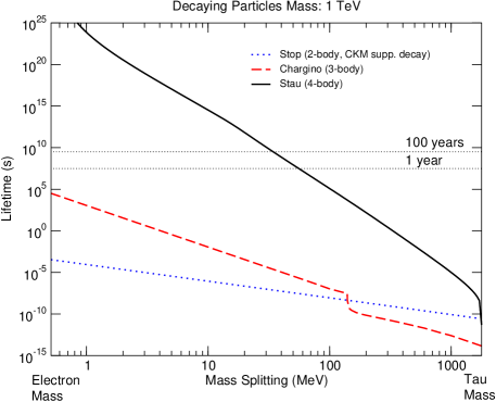
Figure 7: The lifetime of a 1 TeV stop (blue dotted line), a chargino (red dashed line) and a stau (black solid line), as a function of their mass splitting with the lightest SUSY particle, the lightest neutralino.

Reducing the NLSP mass splitting $\Delta m$ one may hope to obtain “cosmologically relevant” NLSP lifetimes. For scalar quarks, this is not quite the case, as two-body final states always dominate, and even for amplitudes that are CKM-suppressed, the scaling with $\Delta m$ is too shallow, and the resulting lifetimes are rather short, even for very small mass splittings.

The situation is slightly more favorable for charginos, whose three-body decay width is approximately equal to

$$\frac{G_{F}^{2}}{(2\pi)^{3}}\frac{16}{15}(\Delta m)^{5}.$$ (15)

At tree level and in the limit of pure Higgsino-like or Wino-like states, the lightest neutralino and lightest chargino are perfectly degenerate in mass. However, when one takes into account loop corrections to the masses, $\Delta m$ usually turns out to be larger than a few tens of MeV; see, e.g., Pierce:1996zz ; Cheng:1998hc . This translates into an absolute upper limit on the chargino lifetime of about $10^{-(2-3)}$ s.

Finally, in the case of sleptons $\tilde{l}$, the interesting regime is when $\Delta m<m_{l}$ and only four-body decays are allowed. For example, for the lightest stau $\widetilde{\tau_{1}}$, the processes

$$\widetilde{\tau_{1}}\,\,\rightarrow\,\,\chi^{0}_{1}\,\nu_{\tau}\,f\,\bar{f}^{\prime},$$ (16)

with

$$(\bar{f}^{\prime},f)=(\bar{\nu}_{\mu},\mu),\,\,(\bar{\nu}_{e},e),\,\,(\bar{u},d),\,\,(\bar{c},s),$$ (17)

where, depending on $\Delta m$, only final states above the kinematic threshold are included. In this case, $\Delta m$ can be safely taken as a free parameter of the theory: in most scenarios the gaugino mass parameter setting the neutralino mass for bino-like neutralinos, and the scalar soft mass parameter setting the stau mass, are usually assumed to be independent; analogously, there are models in which the $\mu$ parameter setting the mass for a Higgsino-like neutralino, and scalar soft mass parameter are unrelated. A similar picture applies to the smuon, though lifetimes start to be enhanced at much smaller mass splittings ($m_{\mu}$ instead of $m_{\tau}$), and it is theoretically difficult to figure out a scenario in which the lightest smuon is lighter than the lightest stau.

The scalings we have sketched are summarized in Fig. 7, where we plot lifetimes for a stop (CKM-suppressed), a chargino, and a stau as a function of $\Delta m$. The decaying-particle masses have been set to 1 TeV, and the $\Delta m$ range is between the electron and the tau mass. The lifetimes of the stop and of the chargino have been computed with SDECAY Muhlleitner:2003vg . Some details on the computation of the stau lifetime are given below. Notice that the scaling of Eq. (14) is accurately reproduced for all cases. The bottom line is that indeed the lightest stau can play the role of the NLDP with a cosmologically relevant lifetime, and that the stau is the only particle in the MSSM for which this can be guaranteed by adjusting only the LDP-NLDP mass splitting.

VII The Relative Abundance of the Charged NLSP

The next step is to determine the relic density of the NLSP and LSP in the early stages of the evolution of the Universe. As we have already mentioned, we are going to consider thermal production. We briefly review here how to compute the evolution of number densities with coannihilation Griest:1990kh ; edsjogondolo .

Consider a setup with $N$ supersymmetric particles $\chi_{1}$, $\chi_{2}$, … $\chi_{N}$, each with mass $m_{i}$ and number of internal degrees of freedom $g_{i}$. The ordering is such that $m_{1}\leq m_{2}\leq\dots\leq m_{N}$. In the evolution equations, the processes that change the number density of SUSY particles $i$ are of three kinds:

$$\begin{array}[]{lcl}{\rm(a)}\;\;\chi_{i}\;\chi_{j}\leftrightarrow X_{a}^{f}\,,&&\forall\;j\,,\\ {\rm(b)}\;\;\chi_{i}\;X_{b}^{i}\leftrightarrow\chi_{j}\;X_{b}^{f}\,,&&\forall\;j\neq i\,,\\ {\rm(c)}\;\;\chi_{j}\leftrightarrow\chi_{i}\;X_{c}^{f}\,,&&\forall\;j>i\,,\end{array}$$ (18)

where $X_{a}$, $X_{b}^{i}$, $X_{b}^{f}$, and $X_{c}^{f}$ are (sets of) standard-model (SM) particles. In practice, the relevant processes one should include are those for SM particles that are in thermal equilibrium. Assuming the distribution function for each particle $k$ is the same as for the equilibrium distribution function,

$$f_{k}(E_{k})\propto f_{k}^{\rm eq}(E_{k})=\frac{1}{\exp(E_{k}/T)\pm 1}\;,$$ (19)

and invoking the principle of detailed balance, the Boltzmann equation for the evolution of the number density of SUSY particle $i$, $n_{i}=g_{i}/(2\pi)^{3}\int d^{3}pf_{i}(E)$, normalized to the entropy density of the Universe, $Y_{i}=n_{i}/s$, as a function of the variable $x\equiv m_{1}/T$ (with $T$ the Universe temperature; this is equivalent to describing the evolution in time) is given by

$$\frac{x}{\hat{g}(x)\;Y_{i}^{\rm eq}}\frac{dY_{i}}{dx} = -\sum_{j}\frac{\langle\sigma_{ij}v_{ij}\rangle\,n_{j}^{\rm eq}}{H}\left(\frac{Y_{i}\,Y_{j}}{Y_{i}^{\rm eq}\,Y_{j}^{\rm eq}}-1\right)-\sum_{j\neq i}\frac{\left[\sum_{X}\langle\sigma_{iX\rightarrow j}v_{iX\rightarrow j}\rangle\,n_{X}^{\rm eq}\right]}{H}\left(\frac{Y_{i}}{Y_{i}^{\rm eq}}-\frac{Y_{j}}{Y_{j}^{\rm eq}}\right)$$

$$+\sum_{j>i}\frac{\Gamma_{j\rightarrow i}}{H}\left(\frac{Y_{j}}{Y_{i}^{\rm eq}}-\frac{Y_{i}\,Y_{j}^{\rm eq}}{(Y_{i}^{\rm eq})^{2}}\right)-\sum_{j<i}\frac{\Gamma_{i\rightarrow j}}{H}\left(\frac{Y_{i}}{Y_{i}^{\rm eq}}-\frac{Y_{j}}{Y_{j}^{\rm eq}}\right)\;.$$

In this equation, analogously to $Y_{k}$, we have defined $Y_{k}^{\rm eq}\equiv n_{k}^{\rm eq}/s$, the ratio of the equilibrium number density of species $k$ (at temperature $x$) to the entropy density. On the left-hand side, we introduced $\hat{g}(x)\equiv[1+T/(3\,g_{\rm eff})\,dg_{\rm eff}/dT]^{-1}$ with $g_{\rm eff}(T)$ being the effective degrees of freedom in the entropy density. The function $\hat{g}(x)$ is close to 1 except for temperatures at which a background particle becomes nonrelativistic. On the right-hand side, the last two terms contain factors in $\Gamma_{k\rightarrow l}$ that label the partial decay width of a particle $k$ in any final state containing the particle $l$; in our discussion they play a role just at late times when NLSPs decay into LSPs, giving the scaling we have used in Eq. (1). The first two terms refer, respectively, to processes of the kind $(a)$ and $(b)$ in Eq. (18), including all possible SM final and initial states. The symbol $\langle\sigma_{ab}v_{ab}\rangle$ indicates a thermal average of the cross section $\sigma_{ab}v_{ab}$; i.e.,

$$\langle\sigma_{ab}v_{ab}\rangle=\frac{1}{n_{a}^{\rm eq}\,n_{b}^{\rm eq}}\int d^{3}p_{a}d^{3}p_{b}f_{a}^{\rm eq}(E_{a})f_{b}^{\rm eq}(E_{b})\sigma_{ab}v_{ab}\,.$$ (21)

As is evident from the form we wrote the Boltzmann equation, interaction rates have to be compared with the expansion rate $H$ of the Universe. In general, over a large range of intermediate temperatures, the $\langle\sigma_{iX\rightarrow j}v_{iX\rightarrow j}\rangle\,n_{X}^{\rm eq}$ terms will be larger than the $\langle\sigma_{ij}v_{ij}\rangle\,n_{j}^{\rm eq}$ terms, since we expect the cross sections to be of the same order in the two cases, but the scattering rates will be more efficient as long as they involve light background particles $X$ with relativistic equilibrium densities $n_{X}^{\rm eq}$ that are much larger than the nonrelativistic Maxwell-Boltzmann–suppressed equilibrium densities $n_{j}^{\rm eq}$ for the more massive particles $j$. This implies that collision processes go out of equilibrium at a smaller temperature, or later time, than pair-annihilation processes. Writing explicitly the expression for $d/dx(Y_{i}/Y_{i}^{\rm eq}-Y_{k}/Y_{k}^{\rm eq})$, in which Maxwell-Boltzmann–suppressed terms and terms in mass splitting over mass scale can be neglected, one finds explicitly that in the limit that collisional rates are much larger than the expansion rate, for any $i$ and $k$, $Y_{i}(x)/Y_{i}^{\rm eq}(x)=Y_{k}(x)/Y_{k}^{\rm eq}(x)$, or equivalently,

$$Y_{i}(x)=\frac{Y(x)}{Y^{\rm eq}(x)}Y_{i}^{\rm eq}(x)\;,$$ (22)

with $Y(x)\equiv\sum_{k}Y_{k}(x)$ and $Y^{\rm eq}(x)\equiv\sum_{k}Y_{k}^{\rm eq}(x)$. At the temperature $T_{cfo}$, when $\sum_{X}\langle\sigma_{iX\rightarrow k}v_{iX\rightarrow k}\rangle\,n_{X}^{\rm eq}\simeq H$, collision processes decouple and the relative number densities become frozen to about

$$\frac{n_{i}(T)}{n_{k}(T)}=\frac{n_{i}^{\rm eq}\left(T_{cfo}\right)}{n_{k}^{\rm eq}\left(T_{cfo}\right)}\simeq\frac{g_{i}}{g_{k}}\left(\frac{m_{i}}{m_{k}}\right)^{3/2}\exp\left(\frac{m_{k}-m_{i}}{T_{cfo}}\right),$$ (23)

up to the time (temperature) at which heavier particles decay into lighter ones.

The sum $Y(x)$ of the number densities has instead decoupled long before. Eq. (23) is the relation that is implemented to find the usual Boltzmann equation Griest:1990kh ; edsjogondolo for the sum over number densities of all species compared to the sum of equilibrium number densities, and that shows that the decoupling for $Y$ occurs when the total effective annihilation rate becomes smaller than the expansion rate, at a temperature $T_{afo}$ that, as mentioned above, is much larger than $T_{cfo}$.

To get an estimate for $T_{cfo}$, we can take, whenever a channel is kinematically allowed, the (very) rough s-wave limit,

$$\sigma_{i\rightarrow k}v_{i\rightarrow k}\sim\sigma_{ik}v_{ik}\sim\langle\sigma_{ik}v_{ik}\rangle\sim\frac{3\cdot 10^{-27}\,{\rm cm}^{3}\,{\rm s}^{-1}}{\Omega_{\chi}h^{2}}\;,$$ (24)

where an approximate relation between annihilation rate and relic density has been used Jungman:1995df . There are then two possibilities depending on whether (i) the background particle $X$ enforcing collisional equilibrium has a mass much larger than the mass splitting $\Delta m$ between the SUSY particles involved, or (ii) the opposite regime holds. In the first case we find that $T_{cfo}\sim m_{X}/(10-15)$, roughly the temperature at which $X$ itself (except for neutrinos) decouples from equilibrium. From Eq. (23) we find that $n_{i}/n_{k}\simeq g_{i}/g_{k}$; i.e., they have comparable abundances. In the opposite case, we find instead that $T_{cfo}\sim\Delta m/(10-15)$ and hence $n_{i}/n_{k}\simeq g_{i}/g_{k}\left(\frac{m_{i}}{m_{k}}\right)^{3/2}\exp\left[(10-15){\rm sign}(m_{k}-m_{i})\right]$; i.e., the abundance of the heavier particle is totally negligible compared to the lighter one.

Long-lived stau NLSPs are kept in collisional equilibrium with neutralinos by scattering on background $\tau^{\pm}$ and emission of a photon. In this case we are clearly in the limit (i), as $m_{\widetilde{\tau_{1}}}-m_{\chi^{0}_{1}}\ll m_{\tau}$. Since the number of internal degrees of freedom for both staus and neutralinos is 2, we find that the fraction of charged dark matter in this model is

$$f_{\phi}=\frac{g_{\widetilde{\tau_{1}}}}{g_{\chi^{0}_{1}}+g_{\widetilde{\tau_{1}}}}=\frac{1}{2}\,.$$ (25)

More carefully, though, this is not a strict prediction of our MSSM setup for a stau NLDP, and should be interpreted just as an upper limit. In fact, if we have other SUSY particles that are quasi-degenerate in mass with the LSP, and if they then coannihilate and decouple from the neutralino at a later time than the stau, either through mode (i) and then immediately decaying into neutralinos (in all explicit examples, the decay into staus is strongly suppressed compared to the decay into neutralinos), or through mode (ii), then $f_{\phi}$ is reduced to

$$f_{\phi}=\frac{g_{\widetilde{\tau_{1}}}}{\sum_{i=1}^{n}g_{i}}.$$ (26)

where the sum in the denominator involves the neutralino, the stau and all SUSY particles with $T_{cfo}$ lower than the $T_{cfo}$ for staus.

In particular, if the lightest neutralino is a nearly-pure higgsino, then the next-to-lightest neutralino will also be a higgsino very nearly degenerate in mass, and the lightest chargino will also be nearly degenerate in mass, with mass splittings possibly smaller than $m_{\tau}$. In this case, charginos and neutralinos will be kept in collisional equilibrium through scatterings on $(\nu_{l},l)$ pairs. At the same time, the collisional decoupling of staus might be slightly delayed because of chargino-stau conversions through the emission of a photon and absorption of a tau neutrino; however this second process has a Yukawa suppression (as we are considering Higgsino-like charginos) compared to the first, and hence it is still guaranteed that the stau decoupling temperature is larger than the chargino $T_{cfo}$ temperature. Since the mass splitting between neutralino and chargino and that between lightest neutralino and next-to-lightest neutralino cannot be smaller than few tens of MeV (due to loop corrections to the masses), decoupling will always happen in mode (ii) and we do not have to worry about possible stau production in their decays. Since $g_{\chi^{+}}=4$, applying the formula in Eq. (26) we find $f_{\phi}=1/5$. In the case of a wino-like lightest neutralino, instead, the only extra coannihilating partner would be the lightest chargino, yielding $f_{\phi}=1/4$. Finally, adding to this picture, e.g., a quasi-degenerate smuon and selectron, $f_{\phi}=1/7$ could be obtained.

VIII Long lived stau NLSPs in sample minimal models

We provide a few examples of well motivated theoretical scenarios where neutralino-stau degeneracy occurs, possibly in connection with further coannihilating partners driving low values of $f_{\phi}$. In surveying the possible models, the criterion we take here is that of the composition of the lightest neutralino in terms of its dominating gauge eigenstate components. We thus outline bino-, higgsino- and wino-like lightest-neutralino benchmark scenarios.

VIII.1 A case with $f_{\phi}=1/2$: Binos in the mSUGRA model

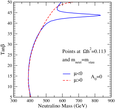
Figure 8: Points of the mSUGRA parameter space, at null trilinear scalar coupling $A_{0}$, featuring $\Omega_{\chi^{0}_{1}}=0.11$ and $m_{\chi^{0}_{1}}=m_{\widetilde{\tau_{1}}}$, for both negative (solid line) and positive (dashed line) sign of the $\mu$ parameter.

As we mentioned above, in the framework of minimal supergravity (mSUGRA) msugra one of the few cosmologically allowed regions of parameter space is the tail where the neutralino and the stau are quasi-degenerate. In this case, coannihilations reduce the exceedingly large bino-like neutralino relic abundance to cosmologically acceptable values for neutralino masses up to around 600 GeV. Coannihilation effects depend on the relative mass splitting between the two coannihilating species. Requiring a mass splitting as small as those found above amounts, as far as the neutralino relic density is concerned, to effectively setting $m_{\chi^{0}_{1}}=m_{\widetilde{\tau_{1}}}$. This, in turns, sets the mass of the neutralino-stau system once a particular value of the relic abundance is required. We plot in Fig. 8 points fulfilling at once $m_{\chi^{0}_{1}}=m_{\widetilde{\tau_{1}}}$ and $\Omega_{\chi^{0}_{1}}=\Omega_{\rm CDM}\simeq 0.113$, the latter being the central value as determined from the analysis of CMB data CMBconstraints . Result are shown in the ($m_{\chi^{0}_{1}}$-$\tan\beta$) plane, with $\tan\beta$ the ratio of the vacuum expectation values of the two neutral components of the $SU(2)$ Higgs doublets, and at a fixed value of the trilinear coupling $A_{0}=0$ (this latter quantity is, however, not crucial here). The solid line corresponds to negative values of the Higgsino mass parameter $\mu$, while the dashed line corresponds to positive values of $\mu$. Notice that at $\mu<0$ the accidental overlap of the heavy Higgs resonance with the coannihilation strip, around $\tan\beta=43$, shifts the neutralino masses to larger values. We point out that the two requirements of mass degeneracy and of the correct relic density determine, at a given value of $\tan\beta$, the required mass of the neutralino-stau system, thus solving the residual mSUGRA parameter space degeneracy, and making the present framework testable and predictive.

In the minimal configuration we have considered, only the lightest neutralino and the lightest stau are playing a role, hence $f_{\phi}=1/2$. However, since the mass splitting between the lightest stau and lightest smuon and selectron is rather small, assuming a slight departure from universality in the scalar sector, two additional quasi-degenerate scalar particles can be obtained and the fraction of charged dark matter reduced to $f_{\phi}=1/4$.

VIII.2 A case with $f_{\phi}=1/5$: Higgsino-like neutralinos

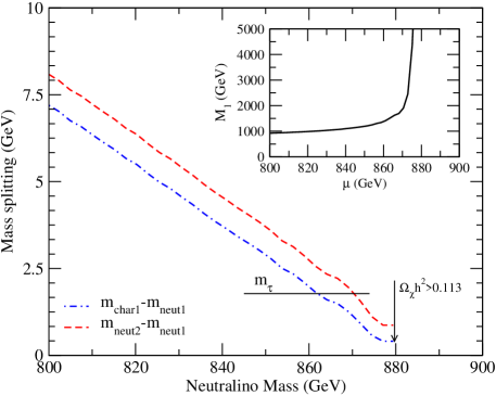
Figure 9: A low-energy parameterization of the higgsino-like neutralino case, at $\tan\beta=50$. In the smaller frame we indicate the points, on the $(\mu,M_{1})$ plane, that give $\Omega h^{2}\simeq 0.113$. The corresponding models are reproduced in the larger frame, where we plot the relevant mass splittings of the chargino-neutralino system.

When the $\mu$ term is lighter than the gaugino masses $M_{1}$ and $M_{2}$, the lightest neutralino gets dominated by the higgsino component. This situation occurs, again within the mSUGRA model, in the so-called hyperbolic branch/focus point (HB/FP) region Chan:1997bi ; Feng:1999zg , where large values of the common soft breaking scalar mass $m_{0}$ drive $\mu$ to low values. In this region, scalars are naturally heavy, at least in the minimal setup; however, the occurrence of non-universalities in the scalar sector Profumo:2003em may significantly affect the sfermion mass pattern. In particular, in a SUSY-GUT scenario, soft breaking sfermion masses get contributions from $D$-terms whenever the GUT gauge group is spontaneously broken with a reduction of rank Drees:1986vd . Light staus may naturally occur, for instance when the weak hypercharge $D$-term dominates and features negative values. In this case the hierarchy between diagonal entries in the soft supersymmetry-breaking scalar mass matrices is $m^{2}_{E}\ll m^{2}_{U,D,Q,L}$. The $m^{2}_{L}$ term may also be lowered in presence of additional $D$-terms originating from the breaking of further $U(1)$ symmetries.

The relic neutralino abundance is here fixed by the interplay of multiple chargino-stau-neutralino coannihilations. In the limit of pure higgsino, the dynamics of these processes fixes the value of $\mu$ yielding a given relic neutralino abundance. On the other hand, a mixing with the bino component along the borders of the HB/FP region may entail a larger spread in the allowed mass range, affecting the $\chi^{0}_{1}$ higgsino fraction. We sketch the situation in Fig. 9, where we resort, for computational ease, to a low-energy parameterization of the above outlined scenario. The smaller frame shows the points on the $(\mu,M_{1})$ plane that produce the required amount of relic neutralinos. The larger frame reproduces the values of the chargino-neutralino and neutralino–next-to-lightest-neutralino mass splitting; the lines end in the pure-higgsino regime. Suitable models, in the present framework, must also fulfill the mass splitting requirement $m_{\widetilde{\chi}_{2},\widetilde{\chi}^{+}_{1}}-m_{\chi^{0}_{1}}<m_{\tau}$. This enforces the allowed neutralino mass range, at $\tan\beta=50$, between 870 and 880 GeV. Had we lowered the value of $\tan\beta$, the corresponding $m_{\chi^{0}_{1}}$ range would only have shifted to masses just a few tens of GeV lighter.

As we have already mentioned, since we are dealing with a case with two neutralinos, a chargino and a stau quasi-degenerate in mass, we find $f_{\phi}=1/5$. Again, a smuon and a selectron can be added to this to shift the charged particle fraction to $f_{\phi}=1/7$.

VIII.3 A case with $f_{\phi}=1/4$: Wino-like neutralinos

A benchmark case where the lightest neutralino is wino-like is instead provided by the minimal Anomaly mediated SUSY breaking (mAMSB) scenario mamsb . In this framework, tachyonic sfermion masses are cured by postulating a common scalar mass term, $m_{0}$. The lightest sfermion turns out to correspond to the lightest stau $\widetilde{\tau_{1}}$ again. The latter, at suitably low $m_{0}$ values, may be degenerate in mass with the lightest neutralino. We performed a scan of the mAMSB parameter space, requiring $m_{\chi^{0}_{1}}\simeq m_{\widetilde{\tau_{1}}}$, and found that the correct relic abundance requires the neutralino masses to lie in the range $1250\lesssim m_{\chi^{0}_{1}}\lesssim 1600$ GeV, with the lower bound holding for small values of $\tan\beta$, while the higher for larger ones. The chargino-neutralino mass splitting is always below the $\tau$ mass, since $\chi^{0}_{1}$ in mAMSB is always a very pure wino, and it has large masses. We finally remark that here, as in the case of higgsinos, the occurrence of stau coannihilations raises the neutralino relic abundance, contrary to the standard result with a bino-like LSP.

Since, in this case, we have one neutralino, a chargino and a stau quasi-degenerate in mass, we find $f_{\phi}=1/4$.

VIII.4 The Stau lifetime

Figure 10: A few Feynman diagrams for four-body final states for the process $\widetilde{\tau_{1}}\,\,\rightarrow\,\,\chi^{0}_{1}\,\nu_{\tau}\,f\,\bar{f}^{\prime},$. Diagram (a) is the dominant diagram; diagrams of type (b) are sub-dominant, and diagrams of type (c) are sub-sub-dominant.

The $\widetilde{\tau_{1}}$ four-body decay proceeds through diagrams of the types sketched in Fig. 10. They come in three sets: those with $W$ exchange, those with $H^{\pm}$ exchange, and those with a sfermion exchange. However, since $\Delta m\equiv m_{\widetilde{\tau_{1}}}-m_{\chi^{0}_{1}}$ is much smaller than any supersymmetric-particle mass, the virtuality of all diagrams except those featuring a $\tau$ exchange (diagrams (a) and (b) in the Figure) is extremely large. Hence all diagrams but those with a $\tau$ exchange will be suppressed by a factor $(m_{\tau}/m_{\rm SUSY})^{4}\sim 10^{-8}$, and the interferences with the dominating diagrams by a factor $(m_{\tau}/m_{\rm SUSY})^{2}\sim 10^{-4}$. Of the two diagrams with a $\tau$ exchange, however, the one with the $H^{\pm}$ exchange has a Yukawa suppressed $H^{\pm}f\bar{f}^{\prime}$ vertex, which gives a suppression, with respect to the $W$-exchange diagram,

$$\sim(m_{\mu}\tan\beta/m_{W})^{2}(m_{\tau}\tan\beta/m_{W})^{2}\sim 10^{-7}-10^{-3}$$

$${\rm for}\ \ \tan\beta=5-50$$ (27)

in the most favorable muonic final channel. Notice that the chirality structure of the couplings entails that no interference between these two diagrams is present. Diagrams with a charged Higgs or a sfermion exchange are moreover further suppressed with respect to those with a $W$ exchange by a factor $(m_{W}/m_{\rm SUSY})^{4}$ which, depending on the SUSY spectrum, can also be relevant.

In this respect, a very good approximation to the resulting stau lifetime is obtained by considering only the first diagram, whose squared amplitude reads

$$|A|^{2}=\sum_{\rm final\,states}\,\frac{16(g_{2}/\sqrt{2})^{4}\,(p_{\nu_{\tau}}\cdot p_{f})}{\left((p_{\tau})^{2}-m_{\tau}^{2}\right)^{2}\left((p_{W})^{2}-m_{W}^{2}\right)^{2}}\times$$

$$\times\Big{[}|V_{R}|^{2}\left(2(p_{\chi^{0}_{1}}\cdot p_{\tau})(p_{\tau}\cdot p_{\bar{f}^{\prime}})-(p_{\tau})^{2}(p_{\chi^{0}_{1}}\cdot p_{\bar{f}^{\prime}})\right)+$$

$$+m_{\tau}^{2}|V_{L}|^{2}(p_{\chi^{0}_{1}}\cdot p_{\bar{f}^{\prime}})-2m_{\chi^{0}_{1}}m_{\tau}{\rm Re}(V_{L}^{*}V_{R})(p_{\tau}\cdot p_{\bar{f}^{\prime}})\Big{]},$$ (28)

with $V_{L,R}$ the left- and right-handed coupling of the $\widetilde{\tau_{1}}$ in the $\widetilde{\tau_{1}}\tau\chi^{0}_{1}$ vertex. The sum is extended over the final states of Eq. (17). For numerical purposes, the four-particles phase space is integrated with the use of the Monte Carlo routine Rambo, with final-state finite-mass corrections for all final states.

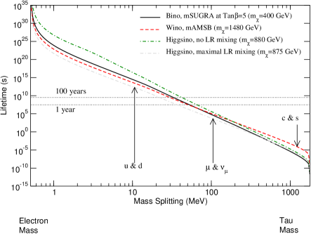
Figure 11: The stau lifetime, as a function of the mass splitting with the lightest neutralino. The parameter space points are defined by the two requirements $m_{\chi^{0}_{1}}\simeq m_{\widetilde{\tau_{1}}}$ and $\Omega_{\chi^{0}_{1}}=0.11$. For the wino and higgsino cases $\tan\beta=50$, while in all cases $A_{0}=0$ and $\mu>0$.

Fig. 11 shows the stau lifetime for a sample of the supersymmetric scenarios outlined in the preceding sections. We fully account for threshold effects in the phase space, with the four contributions from electronic, muonic, and first- and second-generation quarks. The quark masses have been set to their central experimental values Hagiwara:2002fs . For the case of higgsinos, we reproduce the two extreme regimes when the $m^{2}_{L}$ term is large (no Left-Right mixing) and when $m^{2}_{L}\simeq m^{2}_{R}$ (maximal Left-Right mixing). The differences in the lifetimes are traced back to overall mass effects and to the values of the $V_{L}$ and $V_{R}$ couplings (for instance, $|V_{L}|\gg|V_{R}|$ in the wino case, while the opposite regime holds for the case of higgsinos and no LR-mixing). In any case, we conclude that lifetimes of the order of $1-100$ years are obtained with a mass splitting $\Delta m=20-70$ MeV.

IX Dark Matter Searches and Collider Signatures

Unlike other charged long-lived NLDP scenarios, the framework we outlined above has the merit of being, in principle, detectable at dark-matter–detection and collider experiments.

We show in Fig. 12 the spin-independent neutralino-proton scattering cross section for the mSUGRA parameter-space points of Fig. 8, and for the higgsino and wino (mAMSB) cases, as discussed in sec. VIII.2 and VIII.3, together with the current exclusion limits from the CDMS experiment Akerib:2004fq , and the future reach of the XENON 1-ton facility Aprile:2002ef . For binos, at $\mu>0$ most points lie within less than one order of magnitude with respect to the future projected sensitivity, making it conceivable that this scenario may be tested in next-generation facilities. For negative $\mu$, destructive interference among the lightest- and heavy-Higgs contributions lead instead to cancellations in $\sigma_{\chi^{0}_{1}P}$. Finally, higgsino and wino detection rates respectively lie one and two orders of magnitude below the future expected sensitivity.

Indirect-detection experiments look less promising, even for winos and higgsinos, which always feature uncomfortably large neutralino masses. We checked, for instance, that the expected muon flux from the Sun, generated by neutralino pair annihilations, is at most $10^{-(4-5)}$ muons per ${\rm km}^{2}$ per year, far below the sensitivity of future neutrino telescopes like IceCube icecube .

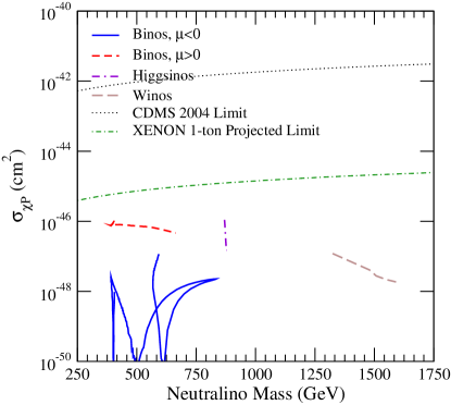
Figure 12: The spin-independent neutralino-proton scattering cross section, as a function of the neutralino mass, along the parameter-space points outlined in Fig. 8. We also indicate the current exclusion limits from the CDMS experiment Akerib:2004fq , and the expected reach of the XENON 1-ton facility Aprile:2002ef .

Turning to collider experiments, considering as the searching tool the usual missing transverse-energy channels, dedicated studies have shown that the mSUGRA coannihilation strip will be within LHC reach, mainly through in a mass range that extends up to $m_{\chi^{0}_{1}}\lesssim 550$ GeV along the coannihilation strip, quite independently of $\tan\beta$ Baer:2003wx . Concerning higgsinos and winos, instead, the relevant mass range we study here appears to be beyond standard LHC searches Baer:2000bs .

Even at high-energy colliders, the peculiar and distinctive feature of this scenario is however represented by the long-lived stau. The production of what have sometimes been dubbed long-lived charged massive particles (CHAMP’s) Acosta:2002ju has been repeatedly addressed. Exclusion limits were determined by the CDF Collaboration Abe:1992vr ; Acosta:2002ju , and the future reach of the LHC and of a future Linear Collider has been also assessed for this broad class of exotic new particles Nisati:1997gb ; Mercadante:2000hw . The case of a stable stau has been, in particular, considered several times, since it occurs in the context of various SUSY-breaking models, like gauge-mediated SUSY-breaking (GMSB) scenarios Giudice:1998bp ; see also, e.g., Ref. Feng:1997zr ; Baer:2000pe . We remark that, contrary to GMSB, in the present framework the production of long lived staus at accelerators is expected to come along together with the production of neutralinos, thus making the two scenarios distinguishable, at least in principle.

A long-lived stau would behave as a highly penetrating particle, appearing in the tracking and muon chambers of collider detectors with a small energy deposit in calorimeters. Staus, depending on their velocities, would produce either highly-ionizing tracks in the low-$\beta$ regime, or, if quite relativistic, they would appear similar to energetic muons. In this latter case, one could look at excesses of dimuon or multi-lepton events as a result of superparticle production; for example, considering the ratio $\sigma(\mu^{+}\mu^{-})/\sigma(e^{+}e^{-})$. In case additional particles have masses close to the neutralino-stau system, the total production cross section of superparticles would be greatly enhanced. Long-lived charginos may also give interesting accelerator signals Feng:1999fu .

While the reach of the Tevatron appears to be insufficient to probe the parameter space of the models we are considering here Feng:1997zr , the discovery of this kind of scenarios at the LHC, though challenging, looks quite conceivable, particularly in the case of binos. In fact, even in the less promising case in which the particle spectrum does not feature any particle close in mass with the $\chi^{0}_{1}-\widetilde{\tau_{1}}$ system, the highly-ionizing–track channel should cover a mass range widely overlapping that indicated in Fig. 8. On the other hand, excess dimuon events could provide an independent confirmation, although the 5-$\sigma$ LHC reach for CHAMP’s in this channel alone has been assessed to lie around 300 GeV Feng:1997zr . Moreover, if additional coannihilating particles (charginos, smuons, or selectrons) are present, the discovery at the LHC would certainly look even more promising Baer:2000pe .

A further recently proposed detection technique for long-lived staus is represented by trapping these particles into large water tanks placed outside the LHC detectors Feng:2004yi . Following the results of Ref. Feng:2004yi , a 10-kton water tank may be capable of trapping more than 10 staus per year, if the mass $m_{\widetilde{\tau_{1}}}\simeq 400$ GeV. The subsequent decays could then be studied in a background-free environment. More than twice as many sleptons would also get trapped in the LHC detectors, although in this case a study of the stau properties would look more challenging Feng:2004yi .

X Conclusions

We have examined a scenario in which a fraction $f_{\phi}$ of the cold-dark-matter component in the Universe is generated in the decay of long-lived charged particles and shown that a scale-dependent (or ‘running’) spectral index is induced. The power spectrum on scales smaller than the horizon size when the age of the Universe is equal to the charged-particle lifetime gets suppressed by a factor $(1-f_{\phi})^{2}$. Such a feature might be singled out unambiguously by future measurements of the power spectrum of neutral hydrogen through the 21-cm line, obtaining direct information on the charged particle lifetime and $f_{\phi}$.

On the contrary, current and future tests for departures from a scale-invariant power spectrum based on Lyman-$\alpha$ data may fail to uniquely identify the scenario we propose. In fact, we have estimated the modifications to the non-linear power spectrum at the redshifts and wavenumbers currently probed by Lyman-$\alpha$ forest data, and shown that these resemble (but are different in detail) those in models with a constant running of the spectral index $\alpha_{s}$. We expect, based on this resemblance, models with $f_{\phi}$ in the range $1/2-1/7$ (as predicted in some explicit models we have constructed) to be compatible with current cosmological data for lifetimes in the range $1-20$ yr. We have also verified that constraints from the primordial light-element abundances and distortions to the CMB spectrum are not violated.

From the particle-physics point of view, we have shown that the proposed scenario fits nicely in a picture in which the lightest neutralino in SUSY extensions of the standard model appears as the cold-dark-matter candidate, and a stau nearly degenerate in mass with the neutralino as the long-lived charged counterpart. A small mass splitting forces the stau to be quasi-stable, since the phase space allowed in the its decay process gets sharply reduced. At the same time, it implies that neutralino and stau are strongly linked in the process of thermal decoupling, with the charged species playing the major role. Owing to these coannihilation effects, the current neutralino thermal relic abundance is compatible with the value inferred from cosmological observatations and, at early times, the stau thermal relic component is at the correct level.

We have described several explicit realizations of this idea in minimal supersymmetric frameworks, including the minimal supergravity scenario, namely the supersymmetric extension of the standard model with smallest possible parameter space. We have pointed out that charged dark matter fraction from 1/2 to 1/7 (or even lower) can be obtained and that stau lifetimes larger than 1 yr are feasible. We have also shown that some of the models we have considered may be detected in future WIMP direct searches, and discussed the prospects of testing the most dramatic feature of the model we propose, i.e. the production of long-lived staus at future high energy particle colliders.

- (1) P. de Bernardis et al., Nature 404, 955 (2000); A. Lange et al., Phys. Rev. D 63, 042001 (2001); S. Hanany et al., Astrophys. J. Lett. 545, L5 (2000); N. W. Halverson et al., Astrophys. J. 568, 38 (2002); B. S. Mason et al., Astrophys. J. 591, 540 (2003); A. Benoit et al., Astron. Astrophys. 399, L2 (2003). D. N. Spergel et al., Astrophys. J. Suppl. 148, 175 (2003).
- (2) A. Gould, B. T. Draine, R. W. Romani, and S. Nussinov, Phys. Lett. B 238, 337 (1990).
- (3) G. D. Starkman, A. Gould, R. Esmailzadeh, and S. Dimopoulos, Phys. Rev. D 41, 3594 (1990).
- (4) E. D. Carlson, M. E. Machacek, and L. J. Hall, Astrophys. J. 398, 43 (1992).
- (5) D. N. Spergel and P. J. Steinhardt, Phys. Rev. Lett. 84, 3760 (2000).
- (6) S. Davidson, S. Hannestad, and G. Raffelt, JHEP 0005, 003 (2000).
- (7) S. L. Dubovsky, D. S. Gorbunov, and G. I. Rubtsov, JETP Lett. 79, 1 (2004) [Pisma Zh. Eksp. Teor. Fiz. 79, 3 (2004)].
- (8) K. Sigurdson, M. Doran, A. Kurylov, R. R. Caldwell, and M. Kamionkowski, Phys. Rev. D 70, 083501 (2004).
- (9) M. S. Turner, Phys. Rept. 197, 67 (1990); G. Raffelt, Phys. Rept. 198, 1 (1990); K. van Bibber and L. Rosenberg, Phys. Rept. 325, 1 (2000).
- (10) G. Jungman, M. Kamionkowski, and K. Griest, Phys. Rept. 267, 195 (1996).
- (11) L. Bergstrom, Rept. Prog. Phys. 63, 793 (2000).
- (12) J. L. Feng, A. Rajaraman, and F. Takayama, Phys. Rev. Lett. 91, 011302 (2003).
- (13) J. L. Feng, S. f. Su, and F. Takayama, arXiv:hep-ph/0404198.
- (14) K. Jedamzik, arXiv:astro-ph/0405583.
- (15) J. L. Feng, A. Rajaraman, and F. Takayama, Phys. Rev. D 68, 063504 (2003).
- (16) K. Sigurdson and M. Kamionkowski, Phys. Rev. Lett. 92, 171302 (2004).
- (17) U. Seljak et al., arXiv:astro-ph/0407372.
- (18) U. Seljak, P. McDonald, and A. Makarov, Mon. Not. Roy. Astron. Soc. 342, L79 (2003).
- (19) M. Tegmark et al. [SDSS Collaboration], Phys. Rev. D 69, 103501 (2004).
- (20) A. Loeb and M. Zaldarriaga, Phys. Rev. Lett. 92, 211301 (2004).
- (21) A. H. Chamseddine, R. Arnowitt, and P. Nath, Phys. Rev. Lett. 49, 970 (1982); R. Barbieri, S. Ferrara, and C. A. Savoy, Phys. Lett. B 119, 343 (1982); L. J. Hall, J. Lykken, and S. Weinberg, Phys. Rev. D 27, 2359 (1983); P. Nath, R. Arnowitt, and A. H. Chamseddine, Nucl. Phys. B 227, 121 (1983).
- (22) L. Randall and R. Sundrum, Nucl. Phys. B 557, 79 (1999); G. F. Giudice, M. A. Luty, H. Murayama, and R. Rattazzi, JHEP 9812, 027 (1998); T. Gherghetta, G. F. Giudice, and J. D. Wells, Nucl. Phys. B 559, 27 (1999).
- (23) C. P. Ma and E. Bertschinger, Astrophys. J. 455, 7 (1995).
- (24) U. Seljak and M. Zaldarriaga, Astrophys. J. 469, 437 (1996).
- (25) R. H. Cyburt, J. R. Ellis, B. D. Fields, and K. A. Olive, Phys. Rev. D 67, 103521 (2003).
- (26) K. Jedamzik, Phys. Rev. Lett. 84, 3248 (2000).
- (27) W. Hu and J. Silk, Phys. Rev. Lett. 70, 2661 (1993).
- (28) J. Fixsen, E. S. Cheng, J. M. Gales, J. C. Mather, R. A. Shafer, and E. L. Wright, Astrophys. J. 473, 576 (1996).
- (29) R. E. Smith et al. [The Virgo Consortium Collaboration], Mon. Not. Roy. Astron. Soc. 341, 1311 (2003).
- (30) J. A. Peacock and S. J. Dodds, Mon. Not. Roy. Astron. Soc. 280, L19 (1996).
- (31) M. J. White and R. A. C. Croft, Astrophys. J. 539, 497 (2000).
- (32) G. Servant and T. M. P. Tait, Nucl. Phys. B 650, 391 (2003).
- (33) K. Griest and M. Kamionkowski, Phys. Rev. Lett. 64, 615 (1990).
- (34) K. Griest and D. Seckel, Phys. Rev. D 43, 3191 (1991).
- (35) J. Edsjo and P. Gondolo, Phys. Rev. D 56, 1879 (1997).
- (36) J. R. Ellis, K. A. Olive, Y. Santoso, and V. C. Spanos, Phys. Lett. B 565, 176 (2003).
- (37) D. M. Pierce, J. A. Bagger, K. T. Matchev, and R. j. Zhang, Nucl. Phys. B 491, 3 (1997).
- (38) H. C. Cheng, B. A. Dobrescu, and K. T. Matchev, Nucl. Phys. B 543, 47 (1999).
- (39) M. Muhlleitner, A. Djouadi, and Y. Mambrini, hep-ph/0311167.
- (40) K. L. Chan, U. Chattopadhyay, and P. Nath, Phys. Rev. D 58, 096004 (1998).
- (41) J. L. Feng, K. T. Matchev, and T. Moroi, Phys. Rev. D 61, 075005 (2000).
- (42) S. Profumo, Phys. Rev. D 68, 015006 (2003).
- (43) M. Drees, Phys. Lett. B 181, 279 (1986).
- (44) K. Hagiwara et al. [Particle Data Group Collaboration], Phys. Rev. D 66, 010001 (2002).
- (45) D. S. Akerib et al. [CDMS Collaboration], astro-ph/0405033.
- (46) E. Aprile et al., astro-ph/0207670.
- (47) J. Edsjö, internal Amanda/IceCube report, 2000.
- (48) H. Baer, C. Balazs, A. Belyaev, T. Krupovnickas, and X. Tata, JHEP 0306, 054 (2003).
- (49) D. Acosta et al. [CDF Collaboration], Phys. Rev. Lett. 90, 131801 (2003).
- (50) F. Abe et al. [CDF Collaboration], Phys. Rev. D 46, 1889 (1992).
- (51) A. Nisati, S. Petrarca, and G. Salvini, Mod. Phys. Lett. A 12, 2213 (1997).
- (52) P. G. Mercadante, J. K. Mizukoshi, and H. Yamamoto, Phys. Rev. D 64, 015005 (2001).
- (53) G. F. Giudice and R. Rattazzi, Phys. Rept. 322, 419 (1999).
- (54) J. L. Feng and T. Moroi, Phys. Rev. D 58, 035001 (1998).
- (55) H. Baer, P. G. Mercadante, X. Tata, and Y. L. Wang, Phys. Rev. D 62, 095007 (2000).
- (56) J. L. Feng, T. Moroi, L. Randall, M. Strassler, and S. f. Su, Phys. Rev. Lett. 83, 1731 (1999).
- (57) H. Baer, J. K. Mizukoshi, and X. Tata, Phys. Lett. B 488, 367 (2000). A. J. Barr, C. G. Lester, M. A. Parker, B. C. Allanach, and P. Richardson, JHEP 0303, 045 (2003).
- (58) J. L. Feng and B. T. Smith, hep-ph/0409278.