A Faraday Rotation Template for the Galactic Sky

Abstract

Using a set of compilations of measurements for extragalactic radio sources we construct all-sky maps of the Faraday Rotation produced by the Galactic magnetic field. In order to generate the maps we treat the radio source positions as a kind of ”mask” and construct combinations of spherical harmonic modes that are orthogonal on the masked sky. As long as relatively small multipoles are used the resulting maps are quite stable to changes in selection criteria for the sources, and show clearly the structure of the local Galactic magnetic field. We also suggest the use of these maps as templates for CMB foreground analysis, illustrating the idea with a cross-correlation analysis between the Wilkinson Microwave Anisotropy Probe (WMAP) data and our maps. We find a significant cross-correlation, indicating the presence of significant residual contamination.

1 Introduction

The origin of large-scale magnetic fields observed on galactic and cluster scales is unknown. The magnetic fields, with observed strengths of $\sim\!10^{-6}$G, could be the consequence of an amplification of a tiny seed ($\la\!10^{-20}$G) by a dynamo mechanism. Alternatively, the compression of a primordial seed ($\sim\!10^{-9}$G) by protogalactic collapse could lead to the fields we see today. Both scenarios require an initial primordial field. Furthermore, the two mechanisms need to explain the high redshift magnetic fields observed in galaxies [Kronberg, Perry & Zukowski 1992] and damped Lyman-$\alpha$ clouds [Wolfe, Lanzetta & Oren 1992]. Magnetic fields play a crucial role in star formation as well as possibly playing an active role in galaxy formation as a whole [Wasserman 1978, Widrow 2002]. Thus, one of the most significant tasks in cosmology is unravelling the mystery behind magnetic fields; from the primordial field to our own Galactic field.

The cosmic microwave background (CMB) provides us with the most distant and extensive probe of the early universe. A primordial magnetic field will leave an imprint in this radiation. Various methods have been developed that seek these signatures. Barrow, Ferreira and Silk (1997) use the anisotropic expansion caused by the presence of a homogeneous primordial field to place limits on its size from large-angle CMB measurements. Others have sought correlation between different scales in the temperature anisotropies [Chen et al. 2004, Naselsky et al. 2004] or computed the effects the field has on the polarisation-temperature cross-correlation [Scannapieco & Ferreira 1997, Lewis 2004]. The existence of a magnetic field at last-scattering also leads to a possible measurable Faraday rotation of the polarised CMB light [Kosowsky & Loeb 1996].

At the other end of the scale, investigation of our own Galaxy’s magnetic field has led to the development of a number of different techniques; Han (2004) provides a concise review of the subject. Techniques include observing Zeeman splitting, polarised starlight, synchrotron radiation, Faraday rotated light and polarised dust emission. However, even with all these methods, there are still outstanding problems. This has led to a lack of consensus on key issues: from the number of spiral arms; how the arms are connected; to the direction the field takes along the arms [Vallée 1997, Han 2004].

To fully understand magnetic fields, we need a coherent picture throughout different epochs. Theories and models can then be tested against this observational picture. A rotation measure (RM) map of the full sky has the potential to fulfil such a goal. RM values probe the integral of the magnetic field from the radiation source to the observer. Obviously, the information encoded in such a map depends on the location of the radiation that is rotated. Faraday rotated polarised CMB radiation will offer both a picture of the primordial field (at the surface of last scattering) and that of our Galaxy. The recent detection of CMB polarisation by DASI [Kovac et al. 2002] and confirmation of this via the Wilkinson Microwave Anisotropy Probe (WMAP; Kogut et al. 2003), have opened up a new avenue in CMB research. Future results from WMAP and Planck satellites will offer polarised data covering the full-sky over a range of frequencies (seven in the case of Planck). By forming a RM map with the data and looking at differing scales, we should be able to untangle the information in the data; on the largest scales the local magnetic field can be studied, whereas the primordial field can be studied on the smaller scales.

On the other hand, one of the main tools for probing local magnetic fields (such as our Galaxy’s) involves utilising RM values from extragalactic sources. Catalogues containing RM values of extragalactic sources have been used to map the Galactic field (eg. Frick et al. 2001). Combining this data with rotation measures from pulsars that are located within our Galaxy, it is conceivable that a 3-dimensional image of the Galactic magnetic field can be built. However, current RM catalogues are both sparsely populated and unevenly sampled. Thus, astute methods are required to produce a RM map with the data at hand.

So, what do we intend to do? We attempt to map the RM values as a function of angular position giving ${\cal R}(\Omega)$, where we use ${\cal R}$ to denote the Faraday rotation measure and $\Omega$ for the angular position. Catalogues containing RM values of extragalactic sources are used to construct the function. The observed spatial distribution of the RM values can be expanded over a set of orthogonal basis functions. For analysis of data distributed on the sky, expansion over spherical harmonics seems natural

$${\cal R}(\Omega)=\sum_{l=1}^{\infty}\sum_{m=-l}^{m=+l}a_{l,m}Y_{l,m}(\Omega),$$ (1)

where the $a_{l,m}$ are the spherical harmonic coefficients and the $Y_{l,m}$ are the spherical harmonics. The properties of the spherical harmonics are well understood and the calculation of the $a_{l,m}$ will allow us to utilise routines within the HEALPix package [Górski, Hivon & Wandelt 1998] for visualisation purposes and further analysis. However, a non-uniform distribution of data points compromises spherical harmonic analysis due to the loss of orthogonality [Górski 1994]. It is more fruitful to analyse a system using orthogonal functions: the statistical properties of the coefficients are simplified. If nonorthogonal functions are used, the properties of the system and the basis are confused. Therefore, we would like to construct an orthonormal basis with functions closely related to those of the spherical harmonics. The spherical harmonic coefficients can then be obtained from the resultant coefficients of the orthonormal basis.

Spherical harmonic analysis of extragalactic sources has been previously performed by Seymour (1966,1984). However, the analysis was carried out using a different form of orthogonalisation and only on a set of 65 sources.

The RM map resulting from our method will be a useful tool for probing Galactic magnetic structure. The map will also be a valuable point of reference when investigating mechanisms that involve the Galactic magnetic field. For example, CMB foregrounds (synchrotron, dust, free-free emission) are correlated with rotation measures [Dineen & Coles 2004]. There is evidence of another foreground component [de Oliveira-Costa et al. 2004], labelled foreground X, that is spatially correlated with $100\mu$m dust emission. Spinning dust grains [Draine & Lazarian 1998] are the most popular candidates for causing this anomalous emission. A RM map can provide insight into the role of these grains as they may align with the local magnetic field. Foreground removal will be particularly challenging in CMB polarisation studies as foregrounds are more dominant than in the temperature anisotropies. Also, single frequency polarisation measurements will not be able to remove the effects of Faraday rotation through the Galactic magnetic field. Thus, the extent to which the results have been effected by the $E$-mode signal rotating into the $B$-mode signal (and vice versa) is unknown.

The layout of the paper is as follows. In the next section we describe the three rotation measure catalogues used in our analysis. In describing the data we clarify the meaning of extragalactic rotation measures. In Section 3 we illustrate a method to generate orthonormal basis functions for each catalogue. From the coefficients of the new basis, the spherical harmonic coefficients are calculated. In Section 4 we present the resulting RM maps and discuss the observed features. In Section 5 we give a brief application of the maps. Correlations are sought between the RM maps and cleaned CMB-only maps. The conclusions are presented and discussed in Section 6.

2 Rotation measure catalogues

Faraday rotation measures of extragalactic radio sources are direct tracers of the Galactic magnetic field. When plane-polarised radiation propagates through a plasma with a component of the magnetic field parallel to the direction of propagation, the plane of polarisation rotates through an angle $\phi$ given by

$$\phi={\cal R}\lambda^{2},$$ (2)

where the Faraday rotation measure is measured in $\mathrm{rad\,m}^{-2}$ where

$${\cal R}=\frac{e^{3}}{2\pi m^{2}_{e}c^{4}}\int n_{e}B_{\parallel}\,ds.$$ (3)

Note that $B_{\parallel}$ is the component of the magnetic field along the line-of-sight direction. The observed RM of extragalactic sources is a linear sum of three components: the intrinsic RM of the source (often small); the value due to the intergalactic medium (usually negligible); and the RM from the interstellar medium of our Galaxy [Broten et al. 1988]. The latter component is usually assumed to form the main contribution to the integral. If this is true, studies of the distribution and strength of RM values can be used to map the Galactic magnetic field [Vallée & Kronberg 1975]. Even if the intrinsic contribution were not small, it could be ignored if the magnetic fields in different radio sources were uncorrelated and therefore simply add noise to any measure of the Galactic field [Frick et al. 2001]. In a similar vein, the distributions of RM values have been used to measure local distortions of the magnetic field, such as loops and filaments, and attempts have also been made to determine the strength of intracluster magnetic fields [Kim, Tribble & Kronberg 1991]. In what follows we shall use RM values obtained from three catalogues in an attempt to map ${\cal R}(\Omega)$ over the whole sky.

All three catalogues are sparsely populated and have non-uniform distributions. It is essential to remove the structure due to the spatial distribution of the sources. This structure is unique to each catalogue. Therefore, for each catalogue a new set of orthonormal functions has to be generated.

The three catalogues used are those of Simard-Normandin et al. (1981; hereafter S81), Broten et al. (1988-updated in 1991; B88) and Frick et al. (2001; F01). S81 present an all-sky catalogue of rotation measures for 555 extragalactic radio sources (ie. galaxies and quasars). B88 and F01 contain 674 and 800 sources respectively. In F01, the two other catalogues are combined with smaller studies of specific regions in the sky (see paper for details). They also provide slightly reduced versions of the other two catalogues. Sources with significantly larger RM values than those in the other studies are removed, leaving catalogues of 551 sources for S81 and 663 for B88. In our analysis we will use these versions of the two catalogues.

Finally, we reject sources with ${\cal R}>300\,\mathrm{rad\,m}^{-2}$. Such large RM values are unlikely to represent real features of the Galactic magnetic field: probably they arise from incorrect determination of ${\cal R}$ due to the $n\pi$ ambiguity in polarisation angle; magnetic fields within the sources; Equation (2) being incorrect; and so on. This final selection criteria reduces the catalogues to 540 sources for S81, 644 for B88, and 744 for F01.

3 Generating a new basis

We can only observe RM values where there happens to be a line of sight. This means we see the RM sky through a peculiar “mask”. We wish to generate a new orthogonal basis that takes account of the spatial structure of this mask. In particular, we need to find a set of functions that are orthogonal on the incomplete sphere. Ideally, these new functions should be related to the spherical harmonics (which are orthogonal functions on a complete sphere). This will enable us to determine the spherical harmonic coefficients from the new functions and their coefficients.

Górski (1994) tackles the problem from the point of view of CMB analysis. The determination of the angular power spectrum is a crucial element of much work in the field. If the temperature anisotropies form a Gaussian random field then they can be completely characterised by the angular power spectrum. In order to obtain the angular power spectrum, one needs to estimate the spherical harmonic coefficients. At low Galactic latitudes ($b<\mathrm{20^{o}}$) foreground contamination is severe. Therefore, it is preferable to obtain an estimate of the spherical harmonic coefficients outside this region. Górski (1994) calculates a new set of functions that are orthogonal to this cut sphere. These functions are used to calculate the spherical harmonic coefficients and thus estimate the angular power spectrum from the two-year COBE-DMR data [Bennett et al. 1994].

In order to see how the method works it is prudent to look at the definition of orthogonal functions. Let us consider two complex functions $A(x)$ and $B(x)$. If

$$\int_{a}^{b}A^{\ast}(x)B(x)\,dx=0,$$ (4)

then $A(x)$ and $B(x)$ are orthogonal over on the interval {$a\,,\,b$}. If we incorporate these two functions into a vector v=[$A(x)$,$B(x)$], the orthogonality of the functions can be expressed through the scalar product

$$\langle{\bf v\cdot v}^{T}\rangle_{\{a,b\}}={\bf I}.$$ (5)

We shall now look at orthogonal functions in the context of a complete sphere. A function can be described by spherical harmonics $Y_{l,m}(\Omega)$ up to an order $l_{\mathrm{max}}$. We can form an $(l_{\mathrm{max}}+1)^{2}$–dimensional vector y=[$Y_{0,0}(\Omega),Y_{1,-1}(\Omega),Y_{1,0}(\Omega),Y_{1,1}(\Omega),\ldots,Y_{l_{\mathrm{max}},l_{\mathrm{max}}}(\Omega)$]. The scalar product is then defined as

$$\langle{\bf y\cdot y}^{T}\rangle_{\{\mathrm{full\>sky}\}}={\bf I}.$$ (6)

The sky can therefore be fully described by

$${\cal R}(\Omega)=\sum_{i=1}^{(l_{\mathrm{max}}+1)^{2}}a_{i}Y_{i}(\Omega)\equiv{\bf a}^{T}\cdot{\bf y}.$$ (7)

However, when the sphere is incomplete due to a Galaxy cut or a more complex mask being applied, we have

$$\langle{\bf y\cdot y}^{T}\rangle_{\{\mathrm{cut\>sky}\}}={\bf W}\neq{\bf I},$$ (8)

where W is the coupling matrix. A new basis, where the equality is true, can be constructed in the following manner. The procedure is a type of Gram-Schmidt orthogonalisation. W can be Choleski-decomposed into a product of a lower triangular matrix L and its transpose

$${\bf W}={\bf L\cdot L}^{T}.$$ (9)

The inverse matrix ${\bf\Gamma}={\bf L}^{-1}$ is then computed. The new set of functions on the cut sky is

$$\psi=\langle{\bf\Gamma\cdot y}\rangle_{\{\mathrm{cut\>sky}\}}.$$ (10)

By construction, we have

$$\langle\psi\cdot\psi^{T}\rangle_{\{\mathrm{cut\>sky}\}} = {\bf\Gamma\cdot y\cdot y}^{T}{\bf\cdot\Gamma}^{T}$$ (11)

$$= {\bf\Gamma\cdot L\cdot L}^{T}{\bf\cdot\Gamma}^{T}$$

$$= {\bf L}^{-1}\cdot{\bf L\cdot L}^{T}\cdot({\bf L}^{-1})^{T}$$

$$= {\bf I}.$$

This can be a useful cross-check for testing the code. Finally, the new basis functions can be used to describe $\cal R$

$${\cal R}(\Omega)=\sum_{i=1}^{(l_{\mathrm{max}}+1)^{2}}c_{i}\Psi_{i}(\Omega)\equiv{\bf c}^{T}\cdot{\bf\psi}.$$ (12)

At this point, only the angular positions $\Omega_{n}$ of the sources have been required. In order to obtain the coefficients $c_{i}$ of the new basis, the rotation measure ${\cal R}_{n}$ themselves are required. It is worth putting it into the context of the data we have. Let the number of sources in our catalogue be $N$ and let $(l_{\mathrm{max}}+1)^{2}\!=\!M$. It should be evident that we have a set of simultaneous equations which have to be solved in order to obtain the coefficients of the new basis functions

$${\cal R}(\Omega_{1}) \!=\! \!c_{1}\psi_{1}(\Omega_{1})+c_{2}\psi_{2}(\Omega_{1})+\ldots+c_{M}\psi_{M}(\Omega_{1})$$

$${\cal R}(\Omega_{2}) \!=\! \!c_{1}\psi_{1}(\Omega_{2})+c_{2}\psi_{2}(\Omega_{2})+\ldots+c_{M}\psi_{M}(\Omega_{2})$$

$$\vdots \vdots$$

$${\cal R}(\Omega_{N}) \!=\! \!c_{1}\psi_{1}(\Omega_{N})+c_{2}\psi_{2}(\Omega_{N})+\ldots+c_{M}\psi_{M}(\Omega_{N}).$$ (13)

So, as long as $N\!>\!M$, these equations should be solvable. Ultimately, we wish to obtain the spherical harmonic coefficients $a_{l,m}$. Using Equation (10), we see

$${\cal R}={\bf a}^{T}\cdot{\bf y}={\bf c}^{T}\cdot{\bf\psi}={\bf c}^{T}\cdot{\bf\Gamma\cdot y}$$ (14)

and therefore

$${\bf a}^{T}={\bf c}^{T}\cdot{\bf\Gamma}\;\rightarrow\;{\bf a}={\bf\Gamma}^{T}\cdot{\bf c}.$$ (15)

So, we have obtained the spherical harmonic coefficients.

There are some practical points that have been glossed over in the above description of the method. Firstly, the RM values in the catalogues need to be smoothed. Otherwise, as the series in Equation (12) is finite, we will be attempting to fit large-scale waves to small-scale features. Ideally, the smoothing will take place in the new basis, however, this is impractical. Therefore, we chose to smooth in harmonic space. Around each source, a hoop of $\mathrm{20^{o}}$ is thrown and the average RM value is taken of the sources within the hoop. This could have been done via a more sophisticated method, say a Gaussian-weighted mean of RM values. However, we chose to use the simple approach. The size of the hoop was chosen to match $l_{\mathrm{max}}$ $(\sim 16)$ closely in angular size. Furthermore, it coincided with the limiting resolution of the wavelet method used in Frick et al. (2001) on the same catalogues.

Secondly, we need to determine to what order we take the series up to, i.e. the value of $l_{\mathrm{max}}$. We do this through trial and error. As we will expand upon in the next section, RM maps were generated for $l_{\mathrm{max}}$ values of 8, 10, 15, 16, 17 and 18. The power spectrum for each map was studied. At some limiting value of $l_{\mathrm{max}}$ the shape at low $l$ alters as features become unstable. Maxima and minima points explode since we are trying to fit more and more function to the same amount of data. That is to say, $N$ is getting too similar to $M$.

Finally, the convention for spherical harmonics has to be chosen carefully. The new basis functions were calculated using the convention of Górski (1994) where

$$Y_{l,m}(\theta,\phi)=\sqrt{\left(\frac{2l+1}{2}\right)}\sqrt{\left(\frac{(l-|m|)!}{(l+|m|)!}\right)}P_{l}^{|m|}(\cos\theta)f(\phi)$$ (16)

and $f(\phi)=\pi^{-1/2}\cos(m\phi),\;(2\pi)^{-1/2}$, or $\pi^{-1/2}\sin(|m|\phi)$ for $m>0,\;=0$, or $<0$. The spherical harmonic coefficients can then be trivially converted into those that adhere to the HEALPix definition of the harmonics where now $f(\phi)=(2\pi)^{-1/2}[\cos(m\phi)+i\sin(m\phi)]$ or $(-1)^{m}(2\pi)^{-1/2}[\cos(m\phi)+i\sin(m\phi)]$ for $m\geq 0$ or $<0$. The convention of Górski (1994) was chosen since the information within the coefficients is more highly compressed. Whereas in the HEALPix definition, the coefficient are complex with a symmetry between +$m$ and -$m$, those following the convention of Górski (1994) are real and contain no such symmetry. The redundant information in the HEALPix coefficients leads to confusion when solving Equation (3).

4 All-Sky RM maps and their Interpretation

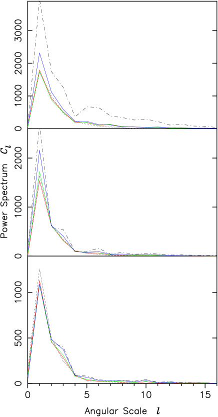
Figure 1: Power spectra (measured in $\mathrm{rad}^{2}\,\mathrm{m}^{-4}$). Red $l_{\mathrm{max}}$=15, green $l_{\mathrm{max}}$=16, blue $l_{\mathrm{max}}$=17, dotted $l_{\mathrm{max}}$=8 and 10, and dash-dot $l_{\mathrm{max}}$=18. From top to bottom: S81, B88 and F01 catalogues.

For all three catalogues, sets of spherical harmonic coefficients were calculated with $l_{\mathrm{max}}$ being set to 8, 10, 15, 16, 17 and 18. From these coefficients, RM maps were produced using the ’synfast’ routine in the HEALPix package. To see whether a RM map was displaying real features or whether the series expansion had been extended too far, we looked at the angular power spectrum of each map. The angular power spectrum is the harmonic space equivalent of the autocovariance function in real space. It is defined as

$$C_{l}=\frac{1}{2l+1}\sum_{m}|a_{l,m}|^{2}.$$ (17)

The spectra of the RM maps are shown in Figure 1. For all three catalogues, it is clear that the shape of the spectra is consistent up to $l_{\mathrm{max}}=16$. Extending the series expansion to higher values of $l_{\mathrm{max}}$ leads to fluctuations in the power on the largest-scales (low $l$). The method finds it harder to reconcile the data with the increasing number of basis functions. The result is that maxima and minima explode as too much freedom is given. This is clearly visible in the maps for $l_{\mathrm{max}}$=17 and 18 (not displayed). Although looking at the bottom sets of spectra for F01, we see the spectra for $l_{\mathrm{max}}$=17 is consistent until the octupole ($l$=3) where it spikes. This suggest that due to the larger data size of F01 it is more able to cope with the demands of increasing the series expansion. Therefore, at times throughout this section, we will focus our analysis on the RM map from the F01 catalogue with $l_{\mathrm{max}}$=16.

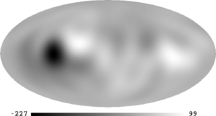
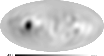
Figure 2: S81 catalogue with 540 sources. Top: $l_{\mathrm{max}}=$10. Bottom: $l_{\mathrm{max}}=$16. All maps are shown in Galactic coordinates with the Galactic centre in the middle and longitude increasing from right to left. The temperature-colour scales are measured in $\mathrm{rad\,m}^{-2}$.

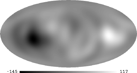
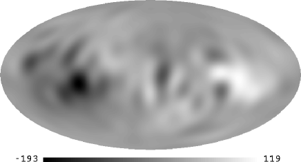
Figure 3: B88 catalogue with 644 sources. Top: $l_{\mathrm{max}}=$10. Bottom: $l_{\mathrm{max}}=$16.

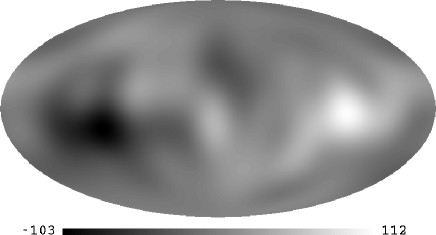
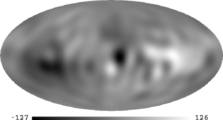
Figure 4: F01 catalogue with 744 sources. Top: $l_{\mathrm{max}}=$10. Bottom: $l_{\mathrm{max}}=$16.

In Figures 2, 3 and 4, we show the RM maps for the S81, B88 and F01 catalogues, respectively. We display only the $l_{\mathrm{max}}$=10 and 16 maps in order not to overload the reader with information. The r.m.s. values of $\cal R$ for the S81, B88 and F01 RM maps ($l_{\mathrm{max}}$=16) are 26.4, 23.5 and 21.5 $\mathrm{rad\,m}^{-2}$, respectively. Maxima (large positive ${\cal R}$) are white, whereas, minima (large negative ${\cal R}$) are black. The two limiting scales enable us to see the progress of structure as the series expansion is extended to include higher modes. We can observe how feature at small $l$ develop as the series extends. Reassuringly, the main features in the $l_{\mathrm{max}}$=16 maps are also present in the $l_{\mathrm{max}}$=10 maps. The positions of the maxima and minima remain roughly unchanged. This is compelling evidence that the observed features are real. However, comparison of the maps from the three catalogues is inhibited by the temperature-colour scale varying from map to map. Therefore, for the $l_{\mathrm{max}}$=16 maps, we force the maximum and minimum scale to be $|{\cal R}|=100\,\mathrm{rad\,m}^{-2}$ ; the results of which are shown in Figure 5.

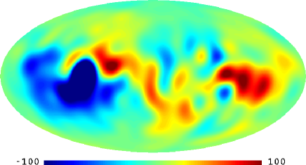
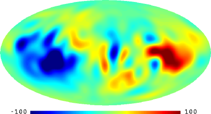
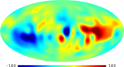
Figure 5: RM maps with identical temperature-colour scaling ($l_{\mathrm{max}}=16$). From top to bottom: S81, B88 and F01 catalogues.

From Figure 5, it is clear that the maxima at $l^{\mathrm{II}}\!\sim\!270^{\mathrm{o}}$ and minima at $l^{\mathrm{II}}\!\sim\!90^{\mathrm{o}}$ are the dominant features in all three plots (here we use $l^{\mathrm{II}}$ to denote Galactic longitude to avoid confusion with the angular scale $l$). This maxima/minima pair corresponds to the large-scale magnetic field in the local Orion spur (sometimes referred to as an arm). These two spots are displaced from the equator to negative Galactic coordinates. This asymmetry between the two hemispheres has been widely reported before (eg. Vallée & Kronberg 1975; Frick et al. 2001); it is usually attributed to the local radio Loop I (the North Galactic spur). Such local distortions are associated with interstellar magnetised superbubbles with typical diameters of 200 pc [Vallée 1997]. There is also a prominent maxima/minima pair towards the Galactic centre in the RM map formed from the F01 catalogue. The centres of the maxima and minima are at $l^{\mathrm{II}}=1^{\mathrm{o}}$ and $l^{\mathrm{II}}=346^{\mathrm{o}}$, respectively . On closer inspection, this feature is present in the RM maps from the other two catalogues. Finally, in the S81 RM map, there is a strong maxima at $l^{\mathrm{II}}\!\sim\!50^{\mathrm{o}}$ in the northern hemisphere. This feature is only suggested in the other two maps.

Figure 6: Galactic equator cross-section ($l_{\mathrm{max}}=16).$Dashed: S81 catalogue; Dotted: B88 catalogue; and Solid line: F01 catalogue

Cross-sections, along the Galactic equator, were taken of the RM maps ($l_{\mathrm{max}}$=16) in order to further understand the features. These are shown in Figure 6. Ideally, with such a slice, maxima/minima locations should indicate the tangential direction to spiral arms and directional field changes should correspond to ${\cal R}\!=\!0$. However, local distortions and flaws in the map-making process, make this not entirely true. The orion spur location is clear for all three maps. Furthermore, the maxima/minima pair towards the Galactic centre (described in the previous paragraph) is evident in all three cross-sections. However, the picture is hazy from $l^{\mathrm{II}}$=30-50^o: there is clear field reversal in S81 map; a hint of a reversal in F01 map; and none in B88 map. The maxima and minima in the cross-sections could be attributed to the named inner arms (eg. the minima near the Galactic centre to the Norma arm), however, this seems quite speculative given the variation from catalogue to catalogue.

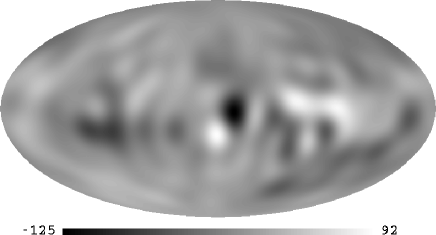
Figure 7: F01 catalogue with both the dipole and quadrupole removed ($l_{\mathrm{max}}=16$).

It is clear that the Orion spur is the dominant feature. Since the associated maxima/minima pair is separated by 180^o, it will be the main source of the dipole ($l$=1). Moreover, we see from the spectra that the quadrupole ($l$=2) is also strong. Therefore, we remove both the dipole and quadruple from the RM map ($l_{\mathrm{max}}$=16) compiled from the F01 data. The results of which are displayed in Figure 7. This enable us to view some of the smaller scale features. These details will be hard to explain solely from Galactic magnetic field models. It will be interesting to see, if these small-scale features persist with larger data sets.

A study of the global Galactic magnetic field structure would benefit from the removal of local distortions. Consequently, we applied the method with the region containing Loop I removed ($b\!>\!0^{\mathrm{o}}$, $0\!<\!l^{\mathrm{II}}\!<\!40^{\mathrm{o}}$, $270\!<\!l^{\mathrm{II}}\!<\!360^{\mathrm{o}}$) [Ruzmaikin & Sokoloff 1977]. However, the removed segment was too large to successfully reconstruct the sky given the remaining sources. The lack of restrictions in the segment meant large maxima/minima formed there. This highlights one disadvantage of spherical harmonic analysis over wavelet analysis that can be localised in both physical and wavenumber spaces. The removal of these local structures is useful for getting a clear picture of the Galactic magnetic field. In CMB foreground studies, however, these structures are essential components of a template.

We now turn to the question of errors in the derived RM maps. In principle there are two distinct types of uncertainty that could arise in the analysis we described above. The first concerns : errors intrinsic to the measurement of ${\cal R}$ and the second relates to errors resulting from sample selection.

We have tackled the first type of error by removing sources with the most extreme values of ${\cal R}$ (those with ${\cal R}>300\,\mathrm{rad\,m}^{-2}$), on the grounds that these are least likely to be galactic. We expect the remaining experimental errors to be stochastic and therefore the process of extracting information on large–scales (as we do) should be unaffected by any underlying noise. The spectrum of this noise should be flat and only dominate on scales where the “real” power is weakest. Experimental errors were addressed in some detail by Frick et al. (2001) in the construction of their catalogue and their versions of the two other catalogues used in our analysis. We feel it would be inappropriate to repeat such a detailed analysis here.

The second type of error corresponds to the sampling uncertainties. This error could be computed reliably if we had a large number of independent samples. This is, of course, impossible but even in cases of non-repeatable observations there are resampling techniques that can be used to make reasonable estimates of these errors. The purpose of resampling the data is to generate further sets with the same population distribution as the original. Small perturbations to the original data set will lead to this. For example, Ling, Frenk & Barrow (1986) apply a ’bootstrap’ resampling technique to estimate the sampling errors in the two–point correlation function estimated from galaxy and cluster redshift data. The bootstrap technique involves sampling $N$ points (with replacement) from the original data set of $N$ sources in order to create pseudo data sets. The variation over an ensemble of such resamplings is used to estimate the error in the statistic in question for the original data. We applied this method to the F01 catalogue with the intention of finding the sample errors in the RM map with $l_{\mathrm{max}}$ set to 16. In total, we produced 50 bootstrap samples from the original data set and from each of these constructed a RM map. The resampling technique is only designed to test the internal variance of the true data set. Mean values obtained from the ensemble of pseudo data sets are not expected to be good estimators of the true mean values. Therefore, from the bootstrap samples, we calculate the standard deviation $\sigma$ at each pixel position $p$

$$\sigma(p)=\sqrt{\sum_{i=1}^{50}\frac{{\cal R}_{i}(p)-\langle{\cal R}(p)\rangle}{49}},$$ (18)

where $i$ corresponds to the bootstrap sample. From this, we constructed a signal–to–noise map where the signal is taken as $|{\cal R}|$ and the noise is $\sigma$. This map is displayed in Figure 8. The map saturates at a signal–to–noise of unity so the regions with low signal to noise are more obvious. The mean signal–to–noise across the whole sky is 117. We found this value to be very stable as the number of bootstrap samples increased and this dictated the number of pseudo data sets produced. Clearly, the majority of the sky is unaffected by sample errors and we feel reassured that the features seen are not the result of sample selection. It appears that the boundaries between positive and negative regions of the sky where the signal is correspondingly low are the most susceptible to sample selection.

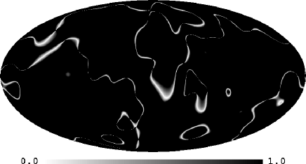
Figure 8: Signal–to–noise map constructed from 50 bootstrap samples of the F01 catalogue. Dark regions are where the estimated signal–to–noise exceeds unity.

The spherical harmonic coefficients generated for all three catalogues with $l_{\mathrm{max}}$ set to 16 are available at http://www.nottingham.ac.uk/~ppxptd/rm_maps. Hopefully, this will enable our method to be compared with other techniques and allow the maps to used in the investigation of observables affected by the Galactic magnetic field. Instructions on the generation of full–sky maps using the HEALPix package are also given at this address.

5 Correlations with CMB maps

As mentioned in the introduction, RM maps have a general importance beyond trying to map the Galactic magnetic field. In what follows, we hope to display one particular function. In this section, we focus solely on the RM map produced from the F01 catalogue with $l_{\mathrm{max}}$ set to 16. Dineen & Coles (2004) developed a diagnostic of foreground contamination in CMB maps. The method measured the cross-correlation between the RM of extragalactic sources and the observed microwave signals at the same angular position. In what follows, we seek correlations between the spherical harmonic modes of the RM map and CMB-only maps. In doing so, we shall look at the phases of the (complex) coefficients of the modes from $l$=2 to $l$=16. Phase correlations have been used before to hunt for evidence of departures in the CMB temperature field from a Gaussian random field [Coles et al. 2004]. In Dineen, Rocha & Coles (2004) a certain form of phase correlation was found to be associated with non-trivial topologies. Phase correlations between CMB and foreground maps have been sought before [Naselsky, Doroshkevich & Verkhodanov 2003, Chiang & Naselsky 2004], however, here we wish to emphasise the virtue of having independent probes of Galactic foreground contamination.

In order to seek evidence of phase correlations between the RM map and CMB data, we turned to two WMAP-derived maps. Both were constructed in a manner that minimises foreground contamination and detector noise, leaving a pure CMB signal. The ultimate goal of these maps is to build an accurate image of the last scattering surface (LSS) that captures the detailed morphology. Following the release of the WMAP 1 yr data, the WMAP team [Bennett et al. 2003], and Tegmark, de Oliveira-Costa & Hamilton (2003; TOH) have released CMB-only sky maps (see papers for details). We use the WMAP team’s internal linear combination (ILC) map and the Wiener-filtered map of TOH. The latter was chosen since the map was found to be correlated with RM values in Dineen & Coles (2004).

Two measures of phase association were used: the circular cross-correlation coefficient $R$ and Kuiper’s statistic $V$. Both statistics will be evaluated at each scale $l$ from 2 to 16. If we let $\Phi_{\mathrm{RM}}$ and $\Phi_{\mathrm{CMB}}$ be the phases of the RM and CMB maps, respectively. Then, following Fisher (1993), $R$ is defined as:

$$R(l)=l^{-1}\sum_{m=1}^{l}\cos(\Phi_{m,\mathrm{RM}}-\Phi_{m,\mathrm{CMB}}).$$ (19)

The expectation value of $R$ is 0, and hence highly correlated phases are associated with large values of $|R|$. Kuiper’s statistic is calculated from the available set of phase differences ($\Phi_{m,\mathrm{RM}}-\Phi_{m,\mathrm{CMB}}$) at a given scale. First, the phase differences are sorted into ascending order, to give the set $\{\Theta_{1},\ldots,\Theta_{p}\}$. Each angle $\Theta_{j}$ is divided by $2\pi$ to give a set of variables $X_{j}$, where $j=1\ldots p$. From the set of $X_{j}$ we derive two values $S^{+}_{p}$ and $S^{-}_{p}$ where

$$S^{+}_{p}={\rm max}\left\{\frac{1}{p}-X_{1},\frac{2}{p}-X_{2},\ldots,1-X_{p}\right\}$$ (20)

and

$$S^{-}_{p}={\rm max}\left\{X_{1},X_{2}-\frac{1}{p},\ldots,X_{p}-\frac{p-1}{p}\right\}.$$ (21)

Kuiper’s statistic is then defined as

$$V(l)=(S^{+}_{p}+S^{-}_{p})\cdot\left(\sqrt{p}+0.155+\frac{0.24}{\sqrt{p}}\right).$$ (22)

The form of $V$ is chosen so that it is approximately independent of sample size for large $p$. Anomalously large values of $V$ indicate a distribution that is more clumped than a uniformly random distribution, while low values mean that angles are more regular.

To access the significance of the values of $R$ and $V$ obtained from the comparison of the RM map with the two CMB maps, we make use of Monte Carlo (MC) skies with uniformly random phases. The statistics were calculated for 10,000 MC skies contrasted with a further 10,000 MC skies. Thus, we are left with 10,000 values of $R$ and $V$ for each scale.

The results from both CMB maps suggests that there is strong correlations between the phases at $l$=11. For the ILC, the values of $R(11)$ and $V(11)$ are greater than 99 percent of the MC values. Whereas, the values of $R(11)$ and $V(11)$ corresponding to the TOH Wiener-filtered map are greater than 97 and 98 percent of the MC skies, respectively. In Figure 9 we plot the ILC map constructed with the $a_{l,m}$ for $l$=11. Overlapping this image with that of the RM in Fig 4, we can see that the central maxima/minima pair in the RM map are similar in location, size and shape to structure in the ILC image (but with colours reversed). This is probably what determines the specific scale $l$=11. Interestingly, $l$=11 corresponds to the scale that Naselsky, Doroshkevich & Verkhodanov (2003) found the greatest level of correlation between the ILC phases and those of the foreground maps.

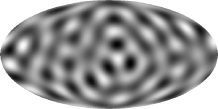
Figure 9: Internal linear combination map constructed with $a_{l,m}$ for $l$=11 only.

6 Conclusion

In this paper, we have presented a new method to generate all-sky RM maps from uneven and sparsely populated data samples. The method calculates a set of functions orthonormal to the data set. With these basis functions, the spherical harmonic coefficients are calculated and converted into sky maps using the HEALPix package. The method was applied to three catalogues; S81, B88 and F01 catalogues. Maps from each catalogue showed evidence of the magnetic field in our local Orion spur, the North-South asymmetry attributed to radio Loop I and a maxima/minima pair close to the Galactic centre that possibly corresponds to the magnetic field of two inner Galactic arms. A RM map constructed from the S81 catalogue also had a prominent maxima at $l^{\mathrm{II}}\!\sim\!50^{\mathrm{o}}$ in the northern hemisphere.

In Section 5, we showed the benefits a RM map has to CMB foreground analysis. Phase correlations were sought between RM maps and those of CMB-only maps derived from the WMAP data. For both the WMAP team’s ILC map and the Wiener-filtered map of TOH, phases corresponding to $l$=11 were found to be highly correlated. Naselsky, Doroshkevich & Verkhodanov (2003) found the same scale to display phase correlations when carrying out a similar analysis on the ILC map and foreground maps. Their detection of correlations at the same scale as our analysis, reaffirms that the RM catalogues are valuable independent tracers of CMB foregrounds [Dineen & Coles 2004].

Modelling foregrounds will play a crucial role in CMB polarisation studies. Foreground contamination is expected to be more severe than in the temperature measurements [Kosowsky 1999]. Consequently, superior templates for the individual foreground components are required. RM maps will help trace these components. Besides this, extrapolation of low frequency measurement of synchrotron polarisation to CMB frequencies has been shown to be complicated by Faraday rotation [de Oliveira-Costa et al. 2003]. Again, this underlines the importance of developing templates of the Faraday rotation of the Galactic sky. Efforts to map the RM sky will be greatly enhanced by increased source catalogues for both extragalactic sources and pulsars within our Galaxy. This may enable the formation of a 3-dimensional image of the Galactic magnetic field. Furthermore, attempts to map the RM sky will be enhanced by upcoming satellite CMB polarisation experiments which present unprecedented sky-coverage and resolution.

References

- [Barrow, Ferreira & Silk 1997] Barrow J.D., Ferreira P.G. & Silk J., 1997, Phys. Rev. Lett., 78, 3610
- [Bennett et al. 1994] Bennett C.L. et al., 1994, ApJ, 436, 423
- [Bennett et al. 2003] Bennett C.L. et al., 2003, ApJS, 148, 97
- [Broten et al. 1988] Broten N.W., MacLeod J.M. & Vallée J.P., 1988, Ap&SS, 141, 303
- [Chen et al. 2004] Chen G., Mukherjee P., Kahniashvili T., Ratra B. & Wang Y., 2004, ApJ, 611, 655
- [Chiang & Naselsky 2004] Chiang L.-Y. & Naselsky P., 2004, astro-ph/0407395
- [Coles et al. 2004] Coles P., Dineen P., Earl J. & Wright D., 2004, MNRAS, 350, 983
- [de Oliveira-Costa et al. 2003] de Oliveira-Costa A., Tegmark M., O’Dell C., Keating B., Timbie P., Efstathiou G. & Smoot G., 2003, Phys. Rev. D, 68, 83003
- [de Oliveira-Costa et al. 2004] de Oliveira-Costa A., Tegmark M., Davies R.D., Gutiérrez C.M., Lasenby A.N., Rebolo R. & Watson R.A., 2004, ApJ, 606, L89
- [Dineen & Coles 2004] Dineen P. & Coles P., 2004, MNRAS, 347, 52
- [Dineen, Rocha & Coles 2004] Dineen P., Rocha G. & Coles P., 2004, submitted to MNRAS, astro-ph/0404356
- [Draine & Lazarian 1998] Draine B.T. & Lazarian A., 1998, ApJ, 494, L19
- [Fisher 1993] Fisher N.I., 1993, Statistical Analysis of Circular Data. Cambridge University Press, Cambridge.
- [Frick et al. 2001] Frick P., Stepanov R., Shukurov A. & Sokoloff D., 2001, MNRAS, 325, 649
- [Górski 1994] Górski K.M., 1994, ApJ, 430, L85
- [Górski, Hivon & Wandelt 1998] Górski K.M., Hivon E. & Wandelt B.D., 1999, in Proceedings of the MPA/ESO Conference Evolution of Large-Scale Structure, eds. A.J. Banday, R.S. Sheth and L. Da Costa, PrintPartners Ipskamp, NL, pp. 37-42 (also astro-ph/9812350)
- [Han 2004] Han J.L., 2004, astro-ph/0402170
- [Kim, Tribble & Kronberg 1991] Kim K.-T., Tribble P.C., Kronberg P.P. 1991, ApJ, 379, 80
- [Kogut et al. 2003] Kogut A. et al., 2003, ApJS, 148, 161
- [Kosowsky 1999] Kosowsky A., 1999, New Astronomy Reviews, 43, 157
- [Kosowsky & Loeb 1996] Kosowsky A. & Loeb A., 1996, ApJ, 469, 1
- [Kovac et al. 2002] Kovac J. M., Leitch E. M., Pryke C., Carlstrom J. E., Halverson N. W. & Holzapfel W. L., 2002, Nature, 420, 772
- [Kronberg, Perry & Zukowski 1992] Kronberg P.P., Perry J.J. & Zukowski E.L., 1992, ApJ, 387, 528
- [Lewis 2004] Lewis A., 2004, accepted by Phys. Rev. D, astro-ph/0406096
- [Ling, Frenk & Barrow 1986] Ling E.N., Frenk C.S. & Barrow J.D., 1986, MNRAS, 223, 21
- [Naselsky, Doroshkevich & Verkhodanov 2003] Naselsky P., Doroshkevich A. & Verkhodanov O., 2003, ApJ, 599, L53
- [Naselsky et al. 2004] Naselsky P.D., Chiang L.-Y., Olesen P. & Verkhodanov O.V., 2004, accepted by ApJ, astro-ph/0405181
- [Ruzmaikin & Sokoloff 1977] Ruzmaikin & Sokoloff, 1977, A&A, 58, 247
- [Scannapieco & Ferreira 1997] Scannapieco E.S. & Ferreira P.G., 1997, Phys. Rev. D, 56, R7493
- [Scóccola, Harari & Mollerach 2004] Scóccola C., Harari D. & Mollerach S., 2004, astro-ph/0405396
- [Seymour 1966] Seymour P.A.H., 1966, MNRAS, 134, 389
- [Seymour 1984] Seymour P.A.H., 1984, QJRAS, 25, 293
- [Simard-Normandin et al. 1981] Simard-Normandin M., Kronberg P. & Button S., 1981, ApJS, 45, 97
- [Sofue & Fujimoto 1983] Sofue Y. & Fujimoto M., 1983, ApJ, 265, 722
- [Tegmark, de Oliveira-Costa & Hamilton 2003] Tegmark M., de Oliveira-Costa A. & Hamilton A., 2003, Phys. Rev. D, 68, 123523
- [Vallée 1997] Vallée J.P., 1997, Fundamentals of Cosmic Physics, 19, 1
- [Vallée & Kronberg 1975] Vallée J.P. & Kronberg P.P., 1975, A&A, 43, 233
- [Wasserman 1978] Wasserman I., 1978, ApJ, 224, 337
- [Widrow 2002] Widrow L.M., 2002, Rev. Mod. Phys., 74, 775
- [Wolfe, Lanzetta & Oren 1992] Wolfe A.M., Lanzetta K.M, & Oren A.L., 1992, ApJ, 388, 17