3D Continuum radiative transfer in complex dust configurations around young stellar objects and active nuclei

Constraints on the density and thermal 3D structure of the dense molecular cloud core $\rho$ Oph D are derived from a detailed 3D radiative transfer modeling. Two ISOCAM images at 7 and 15 $\mu$m are fitted simultaneously by representing the dust distribution in the core with a series of 3D Gaussian density profiles. Size, total density, and position of the Gaussians are optimized by simulated annealing to obtain a 2D column density map. The projected core density has a complex elongated pattern with two peaks. We propose a new method to calculate an approximate temperature in an externally illuminated complex 3D structure from a mean optical depth. This ”$T_{\overline{\tau}}$”-method is applied to a 1.3 mm map obtained with the IRAM 30m telescope to find the approximate 3D density and temperature distribution of the core $\rho$ Oph D. The spatial 3D distribution deviates strongly from spherical symmetry. The elongated structure is in general agreement with recent gravo-turbulent collapse calculations for molecular clouds. We discuss possible ambiguities of the background determination procedure, errors of the maps, the accuracy of the $T_{\overline{\tau}}$-method, and the influence of the assumed dust particle sizes and properties.

1 Introduction

Stars and planetary systems are believed to form within interstellar molecular clouds, from the collapse of condensations of matter often called pre-stellar cores. Despite recent observational and theoretical progress, the physical processes leading to the formation of these cores, and their collapse remain poorly known (e.g. André et al., 2000). The study of pre-stellar cores is essential to the understanding of star formation, since these objects represent the initial conditions of gravitational collapse which influence the subsequent stages of the star-forming process.

1.1 Verification of 1D models of early star formation by observations of molecular cloud cores

In the case of low-mass star-forming regions, it has traditionally been thought that stars form from the inside-out collapse of singular isothermal spheres that are initially in quasi-static equilibrium (Shu et al., 1987), supported against gravity by magnetic and thermal pressure and evolve only due to slow ambipolar diffusion processes (Mouschovias, 1991). In this case, pre-stellar cores at the onset of collapse are expected to follow a $1/r^{2}$ density profile at all radii $r$ (Shu, 1977). Then they collapse dynamically under their own weight and form a protostar, which subsequently accretes matter from its surrounding envelope.

In the last decade, much effort has been put in the understanding of these cold ($T\sim$ 5-15 K) pre-stellar objects, which emit most of their radiation in the (sub)millimeter domain with observations that benefitted from the development of millimeter bolometers, sensitive line detector systems, and infrared cameras. Those observations made it possible to derive line-of-sight integrated properties of the pre-stellar cores. Several studies using (sub-)millimeter continuum (Ward-Thompson et al., 1994; André et al., 1996; Motte et al., 1998; Launhardt et al., 2004) or mid-infrared (MIR) absorption (Bacmann et al., 2000; Abergel et al., 1996) have in particular addressed the density structure. Determining the density structure of pre-stellar objects is fundamental to understand core and protostar evolution, since it has been previously shown that the density structure of pre-stellar objects influences the proto-stellar accretion rate, i.e. after the formation of a central object. According to Henriksen et al. (1997) (see also Foster & Chevalier, 1993), non-singular density profiles in pre-stellar cores lead to accretion rates declining with time in the proto-stellar stage, whereas the accretion rate is expected to be constant if the core has singular $r^{-2}$ profiles (Shu, 1977; Shu et al., 1987).

It was found from the mm and MIR maps that column density profiles of pre-stellar objects are flattened out in their centers. Interpreted by 1D singular isothermal sphere models, the derived density distributions do not follow the $r^{-2}$-profile from the Shu et al. (1987) model, though the profiles do have an $r^{-2}$ part.

The fact that some cores even present sharp edges at large radii ($\sim 0.1$ pc, see Bacmann et al., 2000) tends to show that the reservoir of mass available for subsequent accretion is limited. Therefore to some extent, the density structure of pre-stellar cores must govern stellar masses and influence the initial mass function (Umemoto et al., 2003).

Using the 1D approximation, several types of hydrostatic and quasi-static models have been proposed to account for core formation and evolution. Comparison of the density profiles derived from the observations with the models has been used in order to discriminate between various models (e.g. Ward-Thompson et al., 1994; Ward-Thompson, 1998; André et al., 1996; Bacmann et al., 2000). In most of these studies, circular (or elliptical) averages of the dense core emission (either in the mm or in the MIR) have been performed according to the apparent (projected) geometry of the object. The azimuthal average was also used to increase the signal-to-noise ratio. The profiles thus derived were compared to various power law density models. It was found that the ambipolar diffusion models of magnetically-supported cores provide the best fits, requiring a background magnetic field ranging from 30 to 100 $\mu$G (Wolf et al., 2003).

1.2 Limitations of 1D models of early star formation

Both from observational and from the theoretical side, there are many indications that star formation is an intrinsically three-dimensional process. The profile analysis was often performed in 1D or 2D because of the difficulty of obtaining information along the 3rd dimension, as well as the substantially enhanced numerical effort in 3D star-formation simulations and 3D radiative transfer modeling.

However, the increased sensitivity of bolometer arrays as well as the observations of cores in absorption in the mid-infrared (a technique which is more sensitive to small column densities - e.g. Bacmann et al., 2000; Steinacker et al., 2004) reveals filamentary structures for the cores at large scales, which significantly differ from near-spherical approximations (Apai, 2004). Statistical analyses of core projected shapes (Jones et al., 2001; Jones & Basu, 2002) also tend to show that cores are triaxial. If 1D interpretations represent in simple cases (i.e. for isolated cores) a good approximation of the cores, they can also lead to erroneous density structures, as illustrated by Ballesteros-Paredes et al. (2003). More specifically, Steinacker et al. (2004) used non-symmetric, filamentary density distributions from a smooth particle hydrodynamics simulation of a cloud core evolution to produce MIR and mm maps. By interpreting the absorption maxima in MIR maps and emission maxima mm maps with a 1D model, they found density profiles in ostensible agreement with standard 1D core formation models, but in contradiction to the true underlying non-symmetric distribution.

Moreover, the increased sensitivity and resolution of upcoming telescopes will make it possible to see small-scale structures in these objects and make more sophisticated models more and more necessary. The 3D density structure and eventually its evolution in time is also of crucial interest for chemical models (e.g. Aikawa et al., 2003).

1.3 Gravo-turbulent star formation

The hypothesis that star formation mostly occurs in magnetically subcritical cores and is regulated by slow ambipolar diffusion processes (Shu & Adams, 1987) has been challenged from several sides (see, e.g., the reviews by Larsen, 2003; Mac Low & Klessen, 2004). It is only applicable to isolated, single stars, while it is known that the majority of stars form in small aggregates or large clusters (Adams & Myers, 2001; Lada & Lada, 2003). Furthermore, there is both observational evidence (Crutcher, 2004; André et al., 2000; Bourke et al., 2001; Henning et al., 2001; Wolf et al., 2003) and theoretical reasoning (e.g. Nakano, 1998) that cloud cores do not have magnetic fields strong enough to support the core against gravitational collapse. Also, the long lifetimes implied by the quasi-static phase of evolution in the model are currently discussed regarding, e.g., observational statistics of cloud cores (Taylor et al., 1996; Lee & Myers, 1999; Visser et al., 2002) and chemical age considerations (van Dishoeck & Blake, 1998; Langer et al., 2000). Tassis & Mouschovias (2004), however, have argued that the observational data are consistent with the predictions of the theory of self-initiated, ambipolar-diffusion–controlled star formation.

An alternative to mediation by magnetic fields as controlling agent for stellar birth is supersonic interstellar turbulence (Mac Low & Klessen, 2004). The presence of highly supersonic (and usually super-Alfvénic) turbulent motions in Galactic gas clouds is inferred from molecular line measurements. The observed line widths typically exceed the values for thermal line broadening by far (Blitz, 1993). Only on very small scales and for the so-called quiescent cores does the total linewidth become comparable to the thermal width alone. It is important to note that turbulence usually carries sufficient energy to counterbalance gravity on global scales. The presence of supersonic turbulence therefore prevents contraction of the cloud as a whole. On small scales, however, it may actually provoke localized collapse (Hunter & Fleck, 1982; Elmegreen, 1993; Padoan, 1995; Ballesteros-Paredes et al., 1999; Klessen et al., 2000; Padoan & Nordlund, 1999, 2002; Heitsch et al., 2001). Supersonic turbulence establishes a complex network of interacting shocks, where converging flows generate regions of enhanced density. The compression can be sufficient for local gravitational instability to set in. The same random flow that creates density enhancements in the first place, however, can also disperse them again. For star formation to occur, the localized compression must be fast enough for the contraction region to ‘decouple’ from the flow.

The theory of gravo-turbulent star formation predicts that molecular cloud cores form at the stagnation points of the complex turbulent flow pattern. Their density profiles are constant in the inner region, exhibit an approximate power-law fall-off further out, and usually appear truncated at some maximum radius (see Ballesteros-Paredes et al., 2003). Such configurations closely resemble equilibrium Bonnor-Ebert spheres (Ebert, 1955; Bonnor, 1956), which are popular models for interpreting observed cloud cores. The best studied example probably is the Bok globule B68 (Alves et al., 2001; Lada et al., 2003). However, supersonic turbulence does not create hydrostatic equilibrium configurations. Instead, the density structure is transient and dynamically evolving, as the different contributions to virial equilibrium do not balance (Vázquez-Semadeni et al., 2003). Numerical models predict that gravo-turbulent fragmentation of molecular cloud material will lead to cores that are generally triaxial and in many cases highly distorted. Depending on the projection angle, they often appear extremely elongated, being part of a filamentary structure that may connect several objects (Klessen et al., 2004).

It is the goal of this paper to extend our understanding of pre-stellar cores by entering the complex and difficult world of 3D modeling. The target of our investigation is the pre-stellar core $\rho$ Oph D located in the $\rho$ Ophiuchi star-forming cluster. This core was selected because it has been observed both in the MIR and mm range and the maps indicate a cloud structure deviating from spherical symmetry. We start by outlining the general strategy of the analysis in Sect. 2. In Sect. 3, we present results of a simultaneous fit of ISOCAM images at 7 and 15 $\mu$m by a series of 2D Gaussian profiles to obtain the number column density at each image pixel. The necessary background determination scheme is described and discussed. We compare the derived dust density to an IRAM 30m 1.3 mm map in Sect. 4. Presenting and applying a new method to obtain 3D density and temperature information of cores, we derive constraints on the structure of the core $\rho$ Oph D. A discussion of ambiguities and errors of the obtained distributions is given in Sect. 5. In Sect. 6, we compare the derived spatial distribution with distributions typically obtained in gravo-turbulent simulations and conclude our findings in Sect. 7.

2 General strategy of the 3D analysis

As the 3D analysis of molecular cloud cores based on continuum images is new and includes several steps and approximations, we present in this section a simplified overview of the applied method. Details, tests, and further discussion of single points have been moved to the later sections for clarity.

First, we determine the column density of the core region for each pixel of the 7 and 15 $\mu$m images. In order to estimate the background radiation that is absorbed by the core, we consider the un-absorbed background radiation near the core and interpolate it behind the core. The optical depth is calculated for each pixel and, under the assumption of dust particle size and opacities, converted to a dust column density. To model the 3D distribution of the core, we use a series of 3D Gaussian distributions with axes aligned to the Cartesian axes. The position, the half width at half maximum (HWHM) along the three axis, and the density weight contain 7 free parameters for each Gaussian. To model the column density, the position in the plane of sky, two HWHM, and the weight are varied to fit the images. The corresponding $\chi^{2}$-function is minimized using simulated annealing.

The dust density and temperature distribution along the line of sight is determined by considering mm emission of the dust particles absorbing in the MIR. The emission seen in the 1.3 mm image is obtained from a line-of-sight integral over the emission at each location in the core depending on both the local dust density and temperature. By varying the position and HWHM of the Gaussians along the line of sight, we can fit the 1.3 mm image to obtain the 3D density and temperature structure applying again the simulated annealing optimization algorithm.

The calculation of the dust temperature distribution for a given density distribution requires the application of a 3D continuum radiative transfer (CRT) code. As these computations are far too time-consuming to be repeated many times, we propose and apply an approximative relation to calculate the temperature $T$ at a location in the core from a mean optical depth $\overline{\tau}$ at 7 $\mu$m obtained by a weighted averaging over all directions. This $T_{\overline{\tau}}$-relation is obtained from a few 3D CRT runs covering average and limiting density distributions.

3 Determination of the dust number column density map from ISOCAM maps at 7 and 15 $\mu$m

3.1 Background determination

To obtain a detailed dust column density map of the core, we use the ISOCAM maps from Abergel et al. (1996), which also have been discussed in Abergel et al. (1998). The maps were observed at a central wavelength of $\sim 7$ $\mu$m (LW2 filter [5–8.5 $\mu$m]) and 15 $\mu$m (LW3 filter [12–18 $\mu$m]) with a resolution of $6^{\prime\prime}$. The MIR emission seen in the $\rho$ Oph cloud is thought to arise from very small grains or Polycyclic Aromatic Hydrocarbons (hereafter PAHs) excited on the outside of the cloud by far-UV radiation. The PAHs then re-emit the absorbed energy in the form of spectral bands in the MIR, of which several are encompassed in the ISOCAM filters. Since the extinction in the far-UV is very high and does not penetrate further than $A_{V}\sim 1$ mag, the core itself should be free of PAH emission, the bulk of the observed MIR emission arising from the outer parts of the cloud. For the same reason, emission of the cold dust particles within the core in the 7-15 $\mu$m domain is highly unlikely (the core temperature is lower than 20 K). The radiation received can be modeled as follows (see also Fig. 1):

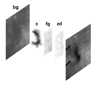
Figure 1: Sketch of the possible layers of matter altering the background radiation on its way through the dense core.

1. A background layer at the origin of excited PAH emission from the outer cloud parts (labeled $bg$), 2. The dense core absorbing this background radiation in the MIR (labeled $c$), 3. A foreground layer similar to the background layer containing absorbing cold dust and a layer of emitting small particles at the border of the cloud ($fg$), and 4. A layer of zodiacal dust with emission and absorption ($zd$). With this approximative decomposition, the total intensity along the line of sight can be written as

$$I_{obs}=\left(I_{bg}\ e^{-\tau_{c}}\ e^{-\tau_{fg}}+I_{fg}+I_{zd}\right)\ e^{-\tau_{zd}}$$ (1)

where $\tau$ is the optical depth.

The $\rho$ Oph cloud is illuminated from behind by the B2V-star HD147889 (Liseau et al., 1999) exciting the PAHs of the background layer. As there is no star in the vicinity of the cloud illuminating the foreground layers, the PAH emission arising from the foreground layer is supposed to be negligible. This is in agreement with the results of Bacmann et al. (2000) who found that the entire foreground emission came from zodiacal dust. The zodiacal dust emission was determined by Abergel et al. (1996) to be 5.7 and 39 MJy/sr for the LW2 (7 $\mu$m) and LW3 (15 $\mu$m) maps, respectively, and has been subtracted from the map. Currently, a possible absorption by cloud dust in front of the core can not be distinguished unambiguously from the core absorption. We note that a small part of the dust distribution derived from the maps might belong to the foreground cloud rather than to the core itself. In that sense, the derived dust densities will be an upper limit to the real densities.

To determine $\tau_{c}$ and the dust column density map, the background behind the core has to be interpolated from the observed background in the vicinity of the core. We assume that the background behind the core follows the gradients that are visible in the maps. After excluding bad pixels containing contamination from previous observations and periodic remnants, we determine a first background approximation by manually masking the core area and interpolating the outer background into the masked area. The background at a given pixel was interpolated as the average of all non-masked pixels within a given radius. This radius was chosen to be 1/3 of the map extent. This reproduces well the background gradient throughout the map without emphasizing local noise features. After having defined this first-order background, we redefine the core area to be the range of pixels where the absorption of this background is larger than $1/e$. Again, the nearby background is interpolated into this new core area. We have verified the stability of the results of our fitting procedure by varying the averaging radius and the size and shape of the initial manually-determined mask of the core area.

3.2 Determination of the optical depth and column density map

The interpretation of the obtained optical depth along lines of sight through the core is ambiguous. The absorption coefficient of dust particles $\kappa$ is a function of their chemical composition $C$, of their size $a$, the temperature $T$, the wavelength $\lambda$, and (via $C$, $a$ and $T$) the location in space. As the temperature range of roughly 5-20 K is small (see, e.g., Stamatellos et al., 2004), we neglect temperature dependencies for the absorption coefficient. As far as dust size is concerned, the dust may grow in the innermost parts of the core changing both its size and chemical composition and hence its optical properties. A mixing of the dust particles due to gas motion countering spatial dependencies is possible but hard to model due to the complex turbulent motions in these cores. A minimum modeling of the dust evolution and the gas motion would be required (see Ossenkopf & Henning, 1994), but it would introduce a wealth of more parameters into the fitting procedure. Since in this paper, we would like to emphasize the detailed structure that was often neglected in former models, we assume that absorption is dominated by dust of a typical size $a$ and refer to a forth-coming paper dealing with a possible spatial variation of the dust size and absorption coefficient.

The dust number column density is calculated by ray-tracing the background intensity through a given spatial 3D dust number density distribution representing the core. There are several useful basis functions that can be used to describe the spatial 3D dust density distribution $n(x,y,z)$ of the core in a series expansion in Cartesian coordinates. Here, we choose a series of $g$ 3D Gaussians with their main axis aligned with the coordinate axis, having the form

$$n(x,y,z)=\sum\limits_{i=1}^{g}G_{i}\exp\left[-d_{i}(x,y,z)\right]$$ (2)

with the argument

$$d_{i}(x,y,z)=\left(\frac{x-x_{i}}{a_{i}}\right)^{2}+\left(\frac{y-y_{i}}{b_{i}}\right)^{2}+\left(\frac{z-z_{i}}{c_{i}}\right)^{2}.$$ (3)

The parameterization contains $7*g$ free parameters (weights $G_{i}$, translations $x_{i}$, $y_{i}$, $z_{i}$, and size parameters $a_{i}$, $b_{i}$, $c_{i}$). This representation has the advantage that the Gaussian profiles are a good approximation for the flattened innermost part of the cores that is seen for many cores (for profiles see, e.g., Bacmann et al., 2000), and include the spherically symmetric case. For the outer parts, the gradients of the density profile have a large uncertainty as projection effects severly change the profiles that are obtained from column density modeling (see, e.g., Steinacker et al., 2004). Therefore, it is currently uncertain if the density follows a powerlaw or an exponential. To keep the inversion method proposed in this paper numerically feasible, we have chosen the number of Gaussians $g$ to be 30, and the implications of this choice are discussed in Sect. 4.2 and Sect. 5.1. We also have tested a series of Gaussians with axes inclined to the line of sight and got the same overall column density distribution with a lower number of Gaussians. The numerical effort is higher, however, since the formula for Gaussians with axes inclined to the line of sight is substantially more complicated. Moreover, for a given number density $n(x,y,z)$, conveniently, the number column density

$$N(y,z) = \int\limits_{-\infty}^{+\infty}dx\ n(x,y,z)$$ (4)

$$= \sqrt{\pi}\sum\limits_{i=1}^{g}a_{i}G_{i}\exp\left[-d(x_{i},y,z)\right]$$ (5)

can be calculated analytically if the line of sight is chosen to be, e.g., along the x-axis. An interclump medium represented by a constant density component has not been added to the density as the Gaussians include this case for large size parameters. Assuming dust particles with an internal density of $\rho_{d}$, the corresponding total dust mass in the core is

$$M=\frac{4}{3}\pi^{5/2}a^{3}\rho_{d}\sum_{i}^{g}G_{i}a_{i}b_{i}c_{i}.$$ (6)

The optical depth between two points $x_{1}$ and $x_{2}$ on the line of sight is

$$\tau_{x}(x_{1},x_{2},y,z,\lambda)=\sigma(\lambda)\int\limits_{x_{1}}^{x_{2}}dx\ n(x,y,z)$$ (7)

with the absorption cross section $\sigma(\lambda)$. For a ray crossing the entire core, we find

$$\tau_{x}(-\infty,\infty,y,z,\lambda)=\sigma(\lambda)N(y,z).$$ (8)

Summing over all pixels k and maps l, we define the $\chi^{2}$-function of the fit to be

$$\chi^{2}=\sum\limits_{l=1}^{m}\sum\limits_{k=1}^{N_{l}}\left(F_{l}(k)-D_{l}(k)\right)^{2}$$ (9)

where $D_{l}$ contains the flux values of each pixel of the two images, $F_{l}$ is the background flux after undergoing absorption due to the model core, $m=2$ is the number of maps, and $N_{l}$ is the number of pixels of map $l$.

The optimization of the 150 parameter dust number density by fitting about 1430 pixels of the MIR maps was performed with a code based on the simulated annealing algorithm (Kirkpatrick et al., 1983; Vanderbilt & Louie, 1984; Thamm et al., 1994; Steinacker & Thamm, 1996; Steinacker & Henning, 2003) which is able to both find minima in the manifold parameter space and to find the deepest minima.

Figure 2: Relative locations and sizes of the individual Gaussians for the optimized number column density distribution. The ellipses are cuts of the Gaussians for $x=x_{i}$ and $n_{i}=G_{i}/e^{2}$. The thick-lined ellipses indicate the most dense Gaussians.

In Fig. 2, the relative location and size of the individual Gaussians is indicated by ellipses having HWHM of size $a_{i}$ and $b_{i}$. The line thickness of the ellipses is logarithmically proportional to the density weight of the Gaussians. The general form of the core is an elongated structure with two peaks and a ratio of projected axis of about 4:1. The larger southern peak is well described by three almost spherical Gaussians. The northern peak has a complex shape and a correct representation of its density structure may require more Gaussians than used in this analysis.

Figure 3: Map of the optical depth $\tau_{x}$ at 7 $\mu$m of the cloud core derived from simultaneously fitting ISOCAM maps at wavelengths of 7 and 15 $\mu$m. Each pixel has a size of 960 AU.

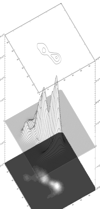
Figure 4: Representations of the number column density of the cloud core derived from simultaneously fitting ISOCAM maps at wavelengths of 7 and 15 $\mu$m.

The number column density map is shown in Fig. 3 as a function of the pixel index of the map (one pixel has a size of 960 AU). The double-peaked structure is pronounced, with the southern peak being the denser part.

In Fig. 4, the optical depth map for 7 $\mu$m is shown as a function of the pixel number. The contours are labeled with the optical depth value $\tau_{x}$ along rays completely crossing the core, reaching a maximum of about 0.5 in the southern maximum and less than 0.4 in the northern maximum. The optical depth does not exceed 0.14 in the region between the two maxima.

Figure 5: ISOCAM images of the dense molecular cloud core $\rho$ Oph D at $\lambda=7\ \mu$m (upper left) and $\lambda=15\ \mu$m (lower left) and maps resulting from fitting all maps with the same number density distribution (right). The white line in the upper left panel indicates a spatial length scale of about 0.13 arcmin or 0.1 pc (20000 AU).

The resulting fit maps using the optimized number density distribution are given in Fig. 5 along with two of the original ISOCAM images (upper and lower left panel shows 7 and 15 $\mu$m, respectively). The white line in the upper left panel represents a spatial scale of about 0.13 arcmin or 0.1 pc (20000 AU). The fit is not able to reproduce the small-scale noise that is part of the real maps but resembles well the overall appearance of the cloud core.

With 30 Gaussian basis functions involved, the fit is ambiguous. The most obvious ambiguity when running the optimization procedure arises from identical density structures where Gaussians just have been exchanged. Moreover, there are several possibilities to arrange the Gaussians to represent the complex extended double-peak structure of such a core. These correspond to different local minima in the parameter space and it requires a special minimization scheme like the simulated annealing algorithm as used in this modeling to find the global minimum of the $\chi^{2}$-function. A more detailed error analysis is given in Sect. 5.

4 Determination of constraints on the 3D density and temperature distribution

4.1 The $T_{\overline{\tau}}$-method

In this section, we want to use a mm map to further constrain the density and temperature distribution of the dust. However, the dust particles absorbing the radiation at 7 and 15 $\mu$m are not obviously the ones dominating emission in the mm range. We assume in first approximation that the absorption and emission is dominated by particles of size a. The absorption in the MIR is described by the optical depth along the line of sight

$$\tau(y,z)=\sigma\int\limits_{-\infty}^{+\infty}n(x,y,z)\ dx=\frac{\sigma\ M_{c}(y,z)}{m_{d}}=\frac{3}{4\rho_{d}}\frac{Q}{a}M_{c}(y,z)$$ (10)

with the total column dust mass $M_{c}$, the dust particle mass $m_{d}$, and the absorption factor $Q$. For pre-stellar cores, the dust sizes are presumably small enough so that the Rayleigh limit $2\pi a\ll\lambda$ is fulfilled for wavelengths around 1 mm and commonly assumed chemical composition of astrophysical dust. Hence, $Q\propto a$, and the optical depth is independent of the dust size as long as the total dust mass is not changed.

The intensity of the mm emission is

$$I_{mm}(y,z)\propto\sigma\int\limits_{-\infty}^{+\infty}n(x,y,z)\ B_{\lambda}[T(x,y,z)]\ dx$$ (11)

where $B$ is the Planck function and $T$ is the temperature of the dust particles (a detailed description of the mm emission is given in Sect. 4.2). The temperature of the dust particles can vary with particle size when the dust is exposed to strong UV and optical radiation. Pre-stellar cores like $\rho$ Oph D are shielded from the short-wavelength part of the spectrum which reduces differences in the dust temperature of different dust sizes. For this application, we assume a temperature depending on the location but not on grain size. Therefore, the emission in the mm is also proportional to the optical depth and it is reasonable to use the spatial dust particle distribution found by fitting maps in the MIR to model the mm emission.

To analyze the mm map, an important parameter is the temperature of the dust in the core with a column density determined from the MIR fit. Temperature distributions of embedded and non-embedded spherically symmetric cores have been calculated by Stamatellos & Whitworth (2003) ranging from 6.5 to 18 K. Zucconi et al. (2001) have discussed both 1D temperature distributions and temperatures in disk-like structures.

The core $\rho$ Oph D clearly has a more complex structure. The temperature of the dust at a certain location $\@vec{x}$ within the core is determined by the local power density balance of incoming and outgoing radiation

$$\int\limits_{0}^{\infty}d\lambda\ 4\pi\ a^{2}\ Q_{abs}(\lambda)\ n(\@vec{x})\ B_{\lambda}[T(\@vec{x})]=$$ (12)

$$\int\limits_{0}^{\infty}d\lambda\ \pi\ a^{2}\ Q_{abs}(\lambda)\ n(\@vec{x})\ \frac{1}{4\pi}\int\limits_{0}^{2\pi}d\phi\int\limits_{0}^{\pi}d\theta\sin\theta\ I(\lambda,\@vec{x},\theta,\phi)$$ (13)

with the intensity $I$ and the direction described in spherical coordinates $\theta$ and $\phi$. Generally, the radiation intensity within the core depends both on the external irradiation and the re-emission of the dust particles, coupling $I$ and $T$ over all wavelengths, locations, and directions. For a complex density structure like the core $\rho$ Oph D, a 3D CRT calculation with self-consistent temperature iteration is required. However, the numerical effort of these codes strongly prohibits any fitting of multi-parameter distributions, as the temperature distribution has to be determined many thousand times in order to find the optimal multi-parameter set in the solution space.

To estimate the range of the temperatures within $\rho$ Oph D, we calculated the radiation field emerging from several density distributions with Gaussians being stretched and translated along the line of sight, but with a fixed extent and column density in the plane of sky to fit the MIR map. The calculations have been performed by a 3D CRT code presented in Steinacker et al. (2003) (see also Steinacker et al., 2002a, b). We followed Zucconi et al. (2001) in assuming an embedding envelope around the core distribution mimicking the true molecular cloud around $\rho$ Oph D. This outer matter shields the core against UV and parts of the optical outer radiation leading to one magnitude of optical extinction. As outer radiation field, the mean interstellar radiation field given in Black (1994), an MIR power law distribution as suggested in Zucconi et al. (2001), and the radiation field of the nearby B2V star were used (Liseau et al., 1999). Numerically, the direction integral was performed using $N_{d}=49$ equally distributed nodes $(\theta_{j},\phi_{j})$ on the unit sphere along with optimized integration weights $\omega_{j}$ (Steinacker & Thamm, 1996).

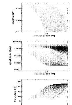
Figure 6: Results from a 3D CRT calculation of the density fitting the MIR maps. The third unknown extent of the single Gaussian was assumed to be the average of the extent in the two other directions. The top panel gives the density of the grid cells as a function of the distance from the southern density peak. The northern density peaks are visible at a distance of about 20000 AU. The middle and lower panel show the limits of the optical depth at 7 $\mu$m and the temperature of the grid cells as function of the distance from the southern density peak, respectively.

Fig. 6 shows results of a first 3D run where we defined for all Gaussians the HWHM along the x-axis (line of sight) to be the mean of the HWHM along the other two axis. A priori, there is no reason to believe that the distribution along x is substantially different from the other two axis, so this is an appropriate first guess. The Gaussians were not translated along the line of sight in this run ($t_{i}=0$). The top plot in Fig. 6 gives the density as a function of the distance to the southern density peak. As the slope of the structure has different gradients in different directions, the distribution broadens quickly towards larger radii, with other maxima at distances of about 20000 AU from the southern peak. The optical depths for all grid points leading from outside the core to the point $\@vec{x}$ along a direction described by the unit vector $\@vec{e}_{\theta,\phi}$ and the parameterization $s$ is

$$\tau_{\theta,\phi}(0,\infty,\lambda)=\sigma(\lambda)\int\limits_{0}^{\infty}ds\ n\left(\@vec{x}-s\@vec{e}_{\theta,\phi}\right).$$ (14)

For $\lambda=7\ \mu$m, the resulting dependency on the distance of $\@vec{x}$ from the southern density maximum is shown in the middle panel of Fig. 6 for all grid cells. Due to the large number of cells and directions, we have plotted, for each grid cell, only the minimal and maximal optical depth when varying the direction. Absorption leads to a maximal optical depth $<$ 2 for photons reaching or crossing the densest part of the core, but again the distribution of possible optical depth is broad. The bottom panel of Fig. 6 gives the temperature at all grid cells as a function of the distance to the density maximum. In the outer parts, $T$ reaches some 15 K, while at the maximal density, it drops below 9 K. Inbetween, temperatures vary strongly depending on the shielding of the different grid cells, and no simple approximation of the temperature can be derived from this plot.

In order to perform a fit of the mm emission of the core density distribution to the observed mm map, an approximative way to find the temperature with moderate numerical effort is required, but not obvious in view of the large spread in the temperature distributions discussed above. In the following, we introduce an approximate method to determine temperatures for pre-stellar cores. Due to the low dust temperatures, the core emits only in the FIR and mm. As the core is optically thin to this emission, we neglect heating of the inner parts by the outer low-density parts. The intensity of the illuminating radiation from the optical to the FIR, therefore, can be written as

$$I(\lambda,\@vec{x},\theta,\phi)=I_{bg}(\lambda)\exp\left[-\tau_{\theta,\phi}(0,\infty,\lambda)\right].$$ (15)

with the background intensity $I_{bg}(\lambda)$. The direction integral on the right-hand side of Eq. (12) can be interpreted as a weighted averaging over different optical depths, so we define a mean optical depth

$$\overline{\tau}(\lambda)\approx-\ln\left\{\sum_{j=1}^{N_{d}}\omega_{j}\exp\left[-\tau_{\theta_{j},\phi_{j}}(0,\infty,\lambda)\right]\right\}.$$ (16)

For a point in space being surrounded by matter with equal column density in all directions, the mean optical depth is identical to the optical depth in any direction as required. For an embedded point in a core with a gap in a certain direction $h$, we correctly find $\overline{\tau}(\lambda)\approx\tau_{\theta_{h},\phi_{h}}(\lambda)$.

Figure 7: Temperature of the grid cells as a function of the mean optical depth at 7 $\mu$m. The solid line indicates the slope of a power law of the form $\tau T^{4}=$const. The dashed line indicates the maximal temperature of grid cells outside the core but inside the cloud.

Fig. 7 gives the relation between the temperature and the mean optical depth at 7 $\mu$m. Hereinafter, we will call this graph the ”$T_{\overline{\tau}}$-diagram”. The relation shows surprisingly little spread. For low optical depth $\overline{\tau}<0.04$, the dust is exposed to the NIR background radiation field and the derived temperature of 15.5 K becomes independent of the absorption (dashed line). For larger optical depth $\overline{\tau}>0.1$, the distribution roughly follows a $\overline{\tau}\sim T^{4}$-law (solid line). This law depends on both the background field $I_{bg}(\lambda)$ and the assumed absorption coefficient $\kappa(\lambda)$. In our case, the re-emission of the dust with a temperature of 7-15 K will occur in the FIR where the assumed absorption law approximately follows $\kappa\propto\lambda^{-2}$. The integral on the left-hand side of Eq. (12) (representing the power density of the radiation emitted by the dust) has then an analytical solution $\propto\zeta(6)\ \Gamma(6)\ T^{6}$ with the zeta function $\zeta$ and the gamma function $\Gamma$. The power density of the incoming radiation on the right-hand side of Eq. (12) contains the sum of two exponentially-dropping contributions from the NIR and FIR peaks of the interstellar radiation field, and is $\sim\overline{\tau}_{7\mu\rm m}^{-6/4}$ for the background field discussed here. This yields the relation $T\sim\overline{\tau}_{7\mu\rm m}^{1/4}$ as seen in Fig. 7. The T($\overline{\tau}$)-correlation can be found for other wavelengths as well. However, for $\lambda<7\ \mu$m, due to the high optical depth, the radiation is no longer contributing substantially to the heating which broadens the distribution. For $\lambda>7\ \mu$m, the relation holds but has more scatter as the dust is absorbing less efficiently.

We will base the following analysis on assuming that the relation established in the $T_{\overline{\tau}}$-diagram will hold even when the detailed 3D structure of the core is changed. The key point is that the heating is mainly related to the mean optical depth and not so much to the actual spatial dust distribution that is leading to this mean optical depth.

Figure 8: Normalized grid cell number at 7 $\mu$m as a function of the temperature for an optical depth of 0.03, 0.05, 0.07, and 0.09, respectively, for 4 different configurations sketched in the inset (30 unperturbed Gaussians, shifted, stretched, and shifted/stretched). The HWHM can be read from the dashed line.

We have tested this assumption by moving and deforming the 30 Gaussian 3D distributions representing our core. The outcome of the calculations is shown for four typical examples in Fig. 8. To test if the $T_{\overline{\tau}}$-relation holds we have plotted the HWHM of the distribution of grid cells having a temperature T, corresponding to vertical cuts through the $T_{\overline{\tau}}$-diagram, for a mean optical depth at 7 $\mu$m of 0.03, 0.05, 0.07, 0.09, respectively. For convenience, the peaks were normalized to 1. The top left panel gives the HWHM for the non-translated and non-perturbed density distribution as derived from the fit of the MIR map and a Gaussian HWHM along the line of sight that is the mean of the two other HWHM of the Gaussians. The right top panel shows the results for a density distribution where we have moved the Gaussians in alternating direction along the line of sight. In the lower left panel, the Gaussians have been stretched by a factor of 2, and in the lower right panel, they were stretched and shifted simultaneously. Evidently, for all four cases, the HWHM of the grid cell distribution are around or less than 1 K, with the trend that stretching of the Gaussians is decreasing the HWHM of the grid cell distribution. The peaks are moved by less than 0.6 K compared to the first case. We conclude that the $T_{\overline{\tau}}$-diagram can be used to determine the temperature approximately from the mean optical depth for all configurations where the Gaussians are shifted and stretched within these limiting cases.

4.2 Fit of the mm map

To fit the 1.3 mm map of $\rho$ Oph D, we applied the background determination method described already for the 7 and 15 $\mu$m maps, and obtained a weak background emission intensity $I_{bg}(y,z)$ in the plane of the sky. The solution of the radiative transfer equation including absorption and emission along a ray parallel to the x-axis is

$$I(+\infty,y,z)=$$ (17)

$$I_{bg}(-\infty,y,z)\ e^{-\sigma(\lambda)N(y,z)}\ +$$ (18)

$$\sigma(\lambda)\int\limits_{-\infty}^{+\infty}dx^{\prime}\ n(x^{\prime},y,z)\ B_{\lambda}[T(x^{\prime},y,z)]\ e^{-\tau_{x}(x^{\prime},+\infty,y,z,\lambda)}.$$ (19)

For wavelengths in the mm range, the optical depth will be small ($\tau_{x}<10^{-4}$) and the exponentials are approximately 1. The solution Eq. (17) contains the unknown number density along the ray $n$ as well as the temperature distribution $T$. Assuming 3D Gaussians with 30 main axes and 30 relative translations along the line of sight, we know the full 3D density $n$. The mean optical depth $\overline{\tau}_{7\mu\rm m}$ can be found and translated into a temperature using the $T_{\overline{\tau}}$-diagram by ray-tracing from different directions. Finally, we integrate along the line of sight according to Eq. (16) to find the intensity. By varying the translation and HWHM of the Gaussians along the line of sight with the simulated annealing technique, we perform a fit of the mm map.

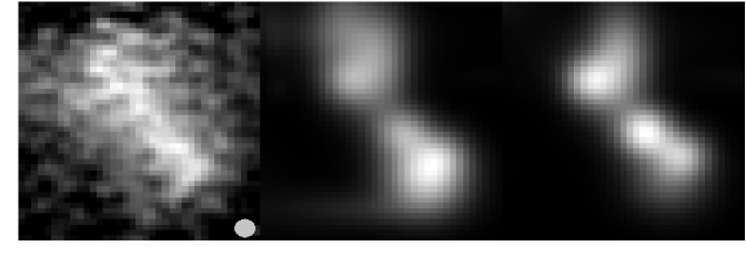
Figure 9: Original 1.3 mm map (left), theoretical map for a column density obtained from the MIR-map fit and a constant temperature of T=10 K (middle), and the fitted map using the $T_{\overline{\tau}}$-relation (right). The grey circle in the left image represents the beam size.

The resulting fit to the mm map is shown in Fig. 9. The left image shows the observed map. Assuming a constant dust temperature of 10 K, the column density map derived from the MIR image can be used to calculate a corresponding mm map (middle image). Aside from the noise of the map, comparison of the map reveals several differences. While the observed map has a more bar-like structure with an approximately constant flux level along the middle of the bar, the mm map for constant temperature has a clear gap between the two main emission maxima seen in MIR. Moreover, the peak flux value of the northern maximum is lower compared to the maximum flux in the lower part of the image. Allowing the program to vary the extent of the Gaussians along the line of sight, the mm emission can be increased by stretching individual clumps. This way, the optical depth to the considered point in space is lowered allowing a more efficient heating and a rise in temperature. While the density is slightly lowered by the stretching, the overall effect is to increase the emissivity. The optimization program therefore stretched the Gaussians in regions where the observed image was brighter, especially in-between the two MIR-emission maxima. Also, the Gaussians forming the maximum in the northern part of the image have been stretched and moved away from each other to decrease the mean optical depth and to increase the emissivity. The right image in Fig. 9 shows the results of shifting and stretching/compressing the Gaussians along the line of sight to fit the mm map. The emission pattern now is more bar-like, but still a gap is visible that cannot be seen in the observed picture. The brightness of the two maxima is equalized, and flux is moved from the southern emission maximum towards the middle structure.

Discussing the deviations, one important point has to be raised in the beginning. A much better fit could be achieved when the Gaussians would be allowed to move in the plane of sky. But as the method is designed to fit both the MIR and mm maps, the Gaussians are fixed in the plane of the sky to enforce a simultaneous fit of the MIR map. This includes that the total mass of each Gaussian is fixed.

The freedom in the fit is reduced due to the limited number of Gaussians, and a better fitting especially in-between the two MIR-emission maxima could be expected from a run with more Gaussians. 3D radiative transfer, even when using the $T_{\overline{\tau}}$-method and combined use of simulated annealing is at the limit of the currently available computer powers so that a substantial increase of the number of Gaussians is not feasible. In addition, the low-resolution mm map used for the fit has a sub-structure that prohibits unambiguous identification of fine-structure in the image. We hope to improve this with upcoming new mm maps. A deeper discussion of the various uncertainties, errors, and approximations is given in the next section.

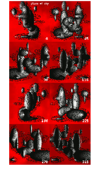
Figure 10: Iso-density surfaces of the 3D dust density structure of the cloud core $\rho$ Oph D at 5% (solid) and 1 % (semi-transparent) of the maximal density for different viewing angles ranging from 0 to 320 degrees with respect to the line of sight seen against an artificial background.

In Fig. 10, we have visualized the 3D dust density structure of the core by showing two iso-density surfaces at 5% (solid surface) and 1 % (semi-transparent surface) of the maximal density and rotating it against an artifical background. The lower density maximum is compact with an extension to model the MIR emission seen in the left lower part of the MIR image. The northern structure is more complex and extended to model both the broader structure seen in the MIR and the high emissivity seen in the mm. In Tab.1, we summarize the overall properties of the cloud.

Table 1: Derived overall properties of the core $\rho$ Oph D

$$\begin{array}[]{p{0.5\linewidth}l}\hline\cr\vskip 3.0pt plus 1.0pt minus 1.0pt\cr Spatial extent&0.22\ {\rm pc}\\ Total gas mass&2.3\ {\rm M}_{\sun}\\ Total gas mass of northern peak&0.8\ {\rm M}_{\sun}\\ Total gas mass of southern peak&1.5\ {\rm M}_{\sun}\\ Maximal density at southern peak&30\ {\rm m}^{-3}\\ Main axes aspect ratio&2:2:1\\ Mean gas density&8\times 10^{-16}\ {\rm kg\ m}^{-3}\\ Temperature range&10-15\ {\rm K}\\ \vskip 3.0pt plus 1.0pt minus 1.0pt\cr\hline\cr\end{array}$$

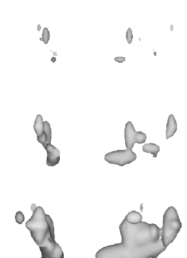
Figure 11: Iso-temperature surfaces of the 3D dust temperature structure of the cloud core $\rho$ Oph D. The left panel shows the distribution seen along the line of sight, while, for the right panel, the view has been rotated by 90^∘. The iso-temperatures are 12 K, 12.8 K, and 13.8 K, respectively (top to bottom).

The 3D dust temperature distribution is visualized in Fig. 11 by showing iso-temperature surfaces for increasing temperature. The left panel gives the view along the line of sight (corresponding to the top left image in Fig. 10), while in the right panel, the configuration is rotated by 90^∘ in a plane perpendicular to the plane of the sky (corresponding to the image with the label ”135” in Fig. 10). The iso-temperatures are 12 K, 12.8 K, and 13.8 K, respectively (top to bottom). In general, the distribution follows the density distribution, as the densest parts are well-shielded and have low temperatures. In the northern part, however, there is a low-temperature region that is not only caused by shielding due to matter around the local density maximum, but also by other nearby local density maxima. This effect becomes important when the density distribution consists of many clumps with comparable maximal density values as in the northern clump. We note that such a realistic temperature distribution including shielding effects can only be obtained doing RT calculations, but that the proposed fast $T_{\overline{\tau}}$-method includes this effect. Animations showing the density and temperature structure are displayed at http://www.mpia-hd.mpg.de/homes/stein/Ani/movief.htm.

5 Ambiguity and error discussion for the 3D modeling

Deriving the complex 3D structure of pre-stellar cores from projected images is a difficult and challenging task. The method and results presented in this paper are a first step to enter this rich 3D world. While the advantage over a 1D or 2D approach is obvious in view of the complex structures of observed cloud cores, the various errors arising from approximations and limited knowledge of the physical conditions make a careful error analysis inevitable. Lacking any analytical solution, however, a quantitative error estimate is often not possible. In turn, many of these errors or ambiguities might be reduced when maps of higher resolution, sensitivity, and dynamical range at the considered wavelengths or images at other wavelengths become available (e.g. by SPITZER, HERSCHEL, JWST, ALMA), or when independent information, e.g., about the background radiation field can be added to the currently available information.

In the following, we will discuss the ambiguities and errors arising from usage of the numerical algorithms, from the approximations and assumptions, and from the observational errors.

5.1 Numerical errors

The column density and emission integrations for given density and temperature distributions are performed with a 5th-order Runge-Kutta scheme incorporating adaptive step size control. The error of this ray-tracing can be neglected compared to the other sources of error.

The density distribution contains 30 three-dimensional Gaussians. In Sect. 6, we already concluded that the number of Gaussians might be too low to resolve the material between the two MIR peaks sufficiently, causing deviations in the mm emission from this region of the core. We did extensive tests including Gaussians with arbitrary orientation in space. Indeed, a smaller number of Gaussians of this type is required to fit a density distribution than for Gaussians with axes along the Cartesian axes. However, the formula for Gaussians with arbitrary orientation in space is substantially more complex increasing the run time of the fitting routine beyond current computer capabilities. We are currently elaborating, if the code can be accelerated by other means to be able to increase the number of Gaussians.

The 3D CRT code has been tested in the framework of the 2D spectral benchmark published in Pascucci et al. (2004), the first benchmark to test five Monte-Carlo and grid/ray-tracing CRT codes by calculating the spectral energy distribution of a star surrounded by a circumstellar dust disk. The deviations of the results for optical depths considered here were below 10%, and most of the deviations were caused by the scattering term, whereas scattering plays no important role for the heating of pre-stellar cores. Nevertheless, we point out that there is no 2D CRT benchmark comparing images nor a 3D CRT benchmark of any kind.

The limitations and possible errors of the proposed $T_{\overline{\tau}}$-method have been discussed already in Sect. 4 for the application to the cloud core $\rho$ Oph D with an approximate total error of about 1 K or less. In general, the method requires to rerun the full 3D CRT code for any newly considered background radiation field in order to obtain the $T_{\overline{\tau}}$-relation. In cases of strong sub-structure of the core material, the number of considered directions for the averaged optical depth might have to be increased. The possible errors arising from additional, but unresolved shielding can be neglected in most cases, but for structures with holes, the method might underestimate the temperature when missing to resolve the illumination through the hole. Comparing the scale of the sub-clumps with the spatial resolution of 1000 AU/pixel for cores in $\rho$ Oph with MIR-instruments like ISOCAM, it is evident, though, that such a strong sub-clumping is currently not observed.

Operating in a complex 210-parameter space, the main question is the ambiguity of the derived optimized parameter set. Optimization algorithms like the gradient search usually succeed in finding a local minimum, but often fail in localizing the deepest minimum of the $\chi^{2}$-function of the fit. For this purpose, more sophisticated methods like simulated annealing or genetic algorithms are applied which have a higher probability in finding the deepest minimum. A prove for completeness is impossible in our case, but from our former experience in applying the method (Thamm et al., 1994; Steinacker & Thamm, 1996; Steinacker & Henning, 2003) as well as from exploring different initial parameter sets, we are confident that the solutions are close to the density structure presented here. Nevertheless, it is correct to state that we can only show that the derived density structure simultaneously fits the three images discussed here, but that we can not exclude that there is another distribution with a comparable $\chi^{2}$-value. We note that the presented density distribution is a valuable working hypothesis for further studies and that we intend to remove some of the ambiguity when more data become available.

The proposed method has another ambiguity that is common in interpreting projected images of 3D configurations. As soon as Gaussians are separated along the line of sight (e.g. when the distance of the maxima is much larger than the HWHM) and not indirectly connected by other Gaussian, there is no way to determine the distance of the clumps. This is because the mm fit uses the temperature difference arising from overlapping Gaussians, and therefore, the temperature is constant for all clumps of large separation. Moreover, separated clumps can be exchanged in their position along the line of sight without changing the observed MIR and mm flux.

For the density structure derived here, this is the case only for a few low-density Gaussians. Hence, we conclude that this ambiguity does not affect the derived distribution of $\rho$ Oph D.

5.2 Approximation and assumption errors

The assumptions concerning dust properties have already been discussed in Sect. 3 and the beginning of Sect. 4. As the total dust mass derived from the MIR maps does not strongly depend on the particle size, we expect the uncertainties in the optical properties of the dust and the gas/dust ratio to dominate the error in the mass. It should be noted that another small error has been introduced by comparing a flux that has been observed through the wavelength filters of ISOCAM to images calculated for a single wavelength. An advanced modeling of the dust properties will be subject to a forthcoming project.

It might be objected that the expansion of the density distribution may cause substantial errors when fitting filamentary structures, especially when inclined to the Cartesian axes. Firstly, the images with the 1000 AU/pixel resolution do not resolve such strongly elongated structures. Secondly, in order to avoid un-physically flat structures, the fitting algorithm allows main axes ratios of up to 10. The maximal ratio obtained in the fits is about 5. Moreover, elongated structures inclined to the Cartesian axes are fitted by several Gaussians with moderate main axes ratios. We therefore argue that the expansion into 3D Gaussians does not produce large fitting errors.

For the determination of the column density from the MIR images, we assume that the invisible background behind the core can be extrapolated from the visible background in the vicinity of the core (the details of the used 2 step-interpolation are given in Sect. 3). The stability of the method was tested by varying interpolation radius and core area. The local variations within the interpolation radius are of the order of 10-15% arising either from variations in the illuminating MIR flux of the photo-dissociation region or from low-density molecular cloud structures along the line of sight.

The exact temperature distribution depends on the assumed properties of the external illuminating radiation field. The 3D radiation field for a core within $\rho$ Oph is not known precisely, as the position within the cloud along the line of sight is unknown, and the MIR flux of the photo-dissociation region and nearby other cores has not been modeled in detail. We note that our approach to have a composition of interstellar radiation field, MIR power law component and nearby B2V star is more realistic than a 1D background field as it is assumed in 1D fits.

5.3 Observational errors

The noise of the MIR images is about 0.3 MJy/sr for the LW2 ISOCAM filter, so that the MIR flux is uncertain to a relative error of less than 10 %. For the mm image, the noise is 6 mJy/13” beam for the core center and the relative flux error is of the order of 15 %.

The simultaneous fit of different images requires an accurate pointing. This is especially valid for the comparison of the MIR and mm image, as the Gaussians are not free to move in the plane of sky when performing the fit to the mm map. An offset would cause the fitting procedure to compensate deviations in position by varying the temperature un-physically. The absolute pointing error in the images was less than 1.4” (2$\sigma$) for the ISO telescope and 3” (1$\sigma$) for the IRAM 30m telescope, which is less than the typically obtained HWHM of the Gaussians.

The technique used for the IRAM 30m 1.3 mm bolometer observations (”dual beam”) is known to filter out some of the extended emissions (e.g. André et al., 1996). Motte & André (2001) have simulated the effects of the dual-beam technique on model objects with intensity profiles following simple power laws and calculated the loss of flux arising in these observations. The flux loss is greater for low power-law indices and increases with increasing radius. We used their modeling to evaluate the flux loss in $\rho$ Oph D and found it to be negligible.

In Sect. 3, we have used a zodiacal light component being constant over the observed area which has an uncertainty of about 20%. Due to the large contribution of the zodiacal light to the total flux and its large error, this foreground flux is dominating the uncertainties in the modeling that arise from observational errors.

6 Comparison with 3D density distributions from gravo-turbulent star-formation models

In the picture of gravo-turbulent star formation, molecular cloud cores are not quasi-static equilibrium objects. Rather they are dynamically evolving as part of the overall turbulent cascade. The same complex and stochastic flow that forms a core at first place continuously reshapes its structure and even may disperse it again. Those cores with an excess of gravitational energy collapse rapidly to form stars, while the others with sufficiently large internal or kinetic energies re-expand once the turbulent compression subsides (Taylor et al., 1996; Vázquez-Semadeni et al., 2004). Consequently, molecular cloud cores are observed having a variety of different shapes, ranging from highly elongated filaments via cometary-shaped structures to very roundish spherically symmetric cores (see e.g. Myers, 1999). This sequence roughly reflects the increasing importance of self-gravity compared to turbulent kinetic energy. Objects that are dominated by turbulent ram pressure tend to have on average more complex morphological appearance than more quiescent cores on the verge of gravitational collapse (Klessen et al., 2004). The latter usually have a rather generic density structure with flat inner profile, followed by an approximate power-law fall-off further out, and apparent truncation at some maximum radius.

The double-peaked and elongated nature of the core $\rho$ Oph D places it somewhere in between these two extremes. Its 3D density structure is typical for pre-stellar cores in their early phases of evolution when the dynamics is still dominated by external compression rather than by self-gravity (Klessen et al., 2004). The relatively small density contrast of about 30 is additional evidence for that. To illustrate this point, Fig. 12 shows the column density map of a typical pre-stellar core in a smooth particle hydrodynamics (SPH) simulation of a self-gravitating supersonically turbulent molecular cloud for comparison (integration along the Cartesian axes).

Figure 12: Column density map of a typical pre-stellar core based on a SPH simulation of a self-gravitating supersonically turbulent molecular cloud. The density is integrated along the three Cartesian axes.

The computation focuses on a cubic volume within the cloud and follows the evolution using smooth particle hydrodynamics (SPH; see Benz, 1990; Monaghan, 1992). This is a particle-based scheme to solve the equations of hydrodynamics well-suited for complex flows with large density contrasts. Turbulence is continuously driven on large scales using a non-local Gaussian field such that the root mean square Mach number is constant (Mac Low, 1999) with value ${\cal M}\approx 6$. Details of the numerical method and associated resolution issues are discussed, e.g., by Klessen & Burkert (2000) and Klessen et al. (2000). The gas is taken to be isothermal with temperature $T=11.3\,$K, corresponding to a sound speed $c_{\rm s}=0.2\,$km s^-1. The computational domain corresponds to a cube of $2.5$ pc length, containing $1140\ M_{\odot}$ of molecular cloud gas. Note, Figure 12 shows only a fraction of $1/103$ of the total volume centered on the considered protostellar core. Complementary aspects of the adopted model are discussed by Ballesteros-Paredes et al. (their model LSD at time $t_{1}$, 2003), Schmeja & Klessen (model M6k2, 2004), Jappsen & Klessen (model M6k2, 2004), and Klessen et al. (model LSD, 2004).

The model core in Fig. 12 is selected because its morphological appearance closely resembles that of $\rho$ Oph D. At the depicted time it is gravitationally unstable and will collapse to build up a protostar during its subsequent evolution. However, due to the highly stochastic nature of compressible turbulent flows the fate of a molecular cloud core is predictable only in a statistical sense. The selected model core, therefore, can at best be indicative of what may happen to $\rho$ Oph D in the next $10^{5}$ years. Nevertheless, it is fair to speculate that gas around the southern density maximum will go into collapse. The fate of the more extended and less dense northern core is hard to predict without further study of possible infall motion. When collapsing into two fragments, the core $\rho$ Oph D would give rise to a wide binary system. A detailed investigation of the dynamical evolution of the core based on the observational data will be the subject of future studies. This will require a combined modeling of the continuum and line data to incorporate velocity informations.

7 Conclusion and Outlook

In this paper, we propose a new method to model the three-dimensional dust density and temperature structure of dense molecular cloud cores. The method is based on the fits of multiple continuum images in which the core is seen in absorption and emission and requires only a few computations with a 3D CRT code. The large parameter space of a three-dimensional structure is covered using simulated annealing as optimization algorithm. One of the key points of the proposed method is the use of a $T_{\overline{\tau}}$-relation that has been derived from the 3D CRT runs. It links the mean optical depth at a given wavelength from outside to a spatial point within the core to the dust temperature at this point, making a fast evaluation of the mm emission along the line of sight possible.

We have applied the method to model the dense molecular cloud core $\rho$ Oph D. In the MIR, the core is seen in absorption against a bright background from the photo-dissociation region of the nearby B2V star, illuminating the cloud from behind. Two ISOCAM images at 7 and 15 $\mu$m have been fitted simultaneously by representing the dust distribution in the core with a series of 3D Gaussian density profiles. The background emission behind the core was interpolated from nearby regions of low extinction. Using simulated annealing, we have obtained a 2D column density map of the core. The column density of the core has a complex elongated pattern with two peaks, with the southern peak being more compact. To retrieve the full three-dimensional structural information, we have calculated the temperature structure of the core with a 3D CRT code, assuming several limiting cases of core extent along the line of sight. It was shown that, for a given position in the core, the relation between the dust temperature and the mean optical depth from outside to this position varies within less than 1 K, when changing the shape of the core along the line of sight. Therefore, the $T_{\overline{\tau}}$-relation was used to estimate quickly the temperature at a given point by a fast direction averaging over the optical depth at just one wavelength. Using this mean, we have varied extent and position of the Gaussian components of the density along the line of sight until a fit of both the MIR and a 1.3mm map, obtained with the IRAM 30m telescope, could be achieved. We have presented the three-dimensional dust density and temperature structure, revealing a condensed southern part and a more extended and complex northern part. We have addressed several sources of errors, namely the background determination method, the assumed dust particle properties, errors in the maps, the ambiguity in the derived distribution, and the approximation error of the $T_{\overline{\tau}}$ method. As we did not reach a perfect fit of the mm image between the two maxima due to the low number of Gaussians, we expect that the detailed 3D structure in-between the density maxima might change when using a higher number of Gaussians. The general structure of a condensed southern maximum and a complex northern multi-clump region, however, is clearly resolved within the limits of the presented analysis. This structure is in general agreement with recent gravo-turbulent collapse calculations for molecular clouds. We speculate that the southern condensation belongs to the category of cloud clumps which are dominated by self-gravity. It may be collapsing to form a star in the near future. The northern clumps, however, may still have sufficiently large internal or kinetic energy to re-expand and merge into the ambient medium once the turbulent compression subsides.

In this application, we determine about 210 free parameter to fit about 2000 pixels simultaneously, but hidden in the assumptions are many more free parameter like the dust properties or details of the illuminating background. It has to be kept in mind, though, that the hidden parameters are present in any other, more simple modeling as well, and often with more unrealistic approximations. The $\rho$ Oph cloud is illuminated from behind in contradiction to a 1D boundary condition for the incoming radiation.

The perspective of applying the method is promising. There are a number of well-observed cores where images at more than two wavelengths are available. With every additional image, the ratio of new unknown background parameter versus constrained parameter decreases, as the density parameters are unchanged. This will increase the accuracy of the determined density structure. Moreover, the derived $T_{\overline{\tau}}$-relations for $\rho$ Oph D can be used in other applications incorporating the temperature.

The ultimate goal of applying the method to well-observed cores, however, will be to address the key question of early star formation, namely if the considered cores have in-falling material. The current line observations provide the molecular line emission flux integrated over all moving gas cells along the line of sight. In the general case, gas motion and emissivity of the cells can not be disentangled, and the 1D approximation or shearing layers are assumed to unfold it. Without unfolding it, infall motion can be mixed up with rotational motion leaving it undecided if the core shows any sign for the onset of star formation. This is changed if the core has been investigated with the $T_{\overline{\tau}}$-method. Knowing the full 3D structure in dust density and temperature, the line of sight-integral can be inverted providing the complete kinematical information if the considered line is optically thin and a model for the depletion of the considered molecules is used. This direct verification of infall motion will be subject to a forthcoming publication.