A new method of measuring the peculiar velocity power spectrum

Abstract

We show that by directly correlating the cluster kinetic Sunyaev Zeldovich (KSZ) flux, the cluster peculiar velocity power spectrum can be measured to $\sim 10\%$ accuracy by future large sky coverage KSZ surveys. This method is almost free of systemics entangled in the usual velocity inversion method. The direct correlation brings extra information of density and velocity clustering. We utilize these information to construct two indicators of the Hubble constant and comoving angular distance and propose a novel method to constrain cosmology.

1. Introduction

The large scale peculiar velocity field, arising from primordial density perturbation, is a fair tracer of the large scale structure of the universe and is of great importance to constrain cosmology and the nature of gravity. But the huge Hubble flow contamination makes its measurement extremely difficult, though several important progresses have been made (e.g. Davis & Peebles (1983); Feldman et al. (2003)). The cluster kinetic Sunyaev Zeldovich (KSZ) effect, which directly measures the cluster peculiar momentum with respect to the CMB, opens a new window for the measurement of the peculiar velocity $v_{p}$ (Haehnelt & Tegmark, 1996; Kashlinsky & Atrio-Barandela, 2000; Aghanim et al., 2001; Atrio-Barandela et al., 2004; Holder, 2004). But the direct inversion of $v_{p}$ requires extra measurements of the cluster Thomson optical depth $\tau$ and cluster temperature. Contaminations in the thermal Sunyaev Zeldovich (TSZ) effect and KSZ measurements and inappropriate assumptions involved in this process put a systematic limit of $\sim 200$ km/s to the inferred $v_{p}$ (Knox et al., 2003; Aghanim et al., 2004; Diaferio et al., 2004).

A natural solution is to avoid the $v_{p}$ inversion, but use the KSZ flux, the direct observable. Contaminations to the cluster KSZ flux have different clustering properties and can be applied to disentangle KSZ signal from contaminations. In the direct correlation estimator of the KSZ flux, many contaminations automatically vanish and most remaining contaminations can be subtracted. We will show that at $z\gtrsim 0.3$, the systematics become sub-dominant and the statistical errors, at $\sim 10\%$ level for South Pole telescope (SPT), dominates. We further derive a novel method, which measures the Hubble constant and comoving distance and thus least model dependent, to constrain cosmology. Throughout this paper, we assume $\Omega_{m}=0.3$, $\Omega_{\Lambda}=1-\Omega_{m}$, $\sigma_{8}=0.9$ and adopt BBKS transfer function (Bardeen et al., 1986).

2. The flux power spectrum

The KSZ cluster surveys directly measure the sum of cluster KSZ flux $S_{\rm KSZ}$ and various contaminations, such as intracluster gas internal flow, radio and IR point sources, primary CMB, cosmic infrared background (CIB), etc. The signal is

$$S_{\rm KSZ}=\frac{\partial B_{T}(\nu)}{\partial T}T_{\rm CMB}\langle\tau\rangle v_{p}\Delta\Omega_{A}=S_{100}v_{100}\ .$$ (1)

Here, $\langle\tau\rangle$ is the $\tau$ averaged over the solid angle $\Delta\Omega_{A}$, $S_{100}$ is the KSZ flux assuming $v_{p}=100{\rm km}/s$ and $v_{100}\equiv v_{p}/100{\rm km}/s$. Since at $\nu\sim 217$ Ghz, the non relativistic TSZ effect, which is one of the major contaminations of the KSZ, vanishes, throughout this paper, we focus on this frequency. At $\nu\sim 217$Ghz, $\partial B/\partial T=540\ {\rm Jy}\ {\rm sr}^{-1}\ {\rm uK}^{-1}$.

Optical follow up of KSZ surveys such as dark energy survey will measure cluster redshift $z$ with uncertainty $\lesssim 0.005$. The $z$ information allows the measurement of 3D correlation

$$\xi_{S}(r) \equiv \langle(S_{i}-\bar{I}\Delta\Omega_{i})(S_{j}-\bar{I}\Delta\Omega_{j})\rangle$$

$$= \langle S_{{\rm KSZ},i}S_{{\rm KSZ},j}\rangle+\cdots\ .$$

Here, $\bar{I}=\sum S_{i}/\sum\Delta\Omega_{i}$ and $\Delta\Omega$ is the solid angle of each cluster. In the correlation estimator, many contaminations such as internal flow and instrumental noise vanish. The majority of remaining systematics can be subtracted directly and the residual systematics is generally (much) less than the statistical errors (§3).

Since $\langle S_{\rm KSZ}S_{\rm KSZ}\rangle$ is cluster number weighted and since $v_{100}$ is correlated at large scale, the corresponding KSZ power spectrum $\Delta^{2}_{\rm KSZ}$ has contributions from both the velocity power spectrum $\Delta^{2}_{v_{100}}$ and the power spectrum $\Delta^{2}_{\delta v\delta v}$ of $\langle\delta_{1}v_{1}\delta_{2}v_{2}\rangle$, where $\delta$ is the matter overdensity. We then have

$$\Delta^{2}_{\rm KSZ}(k) = \left(\int_{m_{\rm low}}S_{100}(m)\frac{dn}{dm}dm\right)^{2}\Delta^{2}_{v_{100}}(k)$$

$$+ \left(\int_{m_{\rm low}}S_{100}(m)b_{n}(m)\frac{dn}{dm}dm\right)^{2}\Delta^{2}_{\delta_{1}v_{1}\delta_{2}v_{2}}\ .$$

Here, $dn/dm$ is the cluster mass function. Throughout this paper, we assume a unity velocity bias and cluster number density bias $\langle b_{n}\rangle=3$. $\Delta^{2}_{v_{100}}$ is given by the linear theory prediction

$$\Delta^{2}_{v_{100}}(k)=\frac{1}{3}\beta^{2}E^{2}(a)a^{2}\frac{\Delta^{2}_{\rm DM}(k,z)}{k^{2}}\ .$$ (4)

Here, $k$ is in unit of $h/$Mpc and $\beta\equiv(a/D)dD/da$ where $D$ is the linear density growth factor. $E(a)$ is the evolution of Hubble constant normalized to $E(a=1)=1$. $\Delta^{2}_{\rm DM}$ is the dark matter power spectrum (variance). We have assumed that two lines of sight are parallel to each other. For less than $10^{\circ}$ angular separation, the accuracy of this assumption is better than $\sim 1\%$. Because of the large bias $\langle b_{n}\rangle$, the $\langle\delta_{1}v_{1}\delta_{2}v_{2}\rangle$ term becomes dominant even in the linear regime at $k\gtrsim 0.06h/$Mpc. Because the nonlinear scale at $z\sim 1$ is $k\simeq 0.5h/$Mpc, we can still using the perturbation theory to predict

$$\Delta^{2}_{\delta_{1}v_{1}\delta_{2}v_{2}}({\bf k}) = \frac{1}{6}\beta^{2}E^{2}(a)a^{2}\frac{k^{3}}{2\pi^{2}}\times$$

$$\int P_{\rm DM}(|{\bf k}-{\bf k}_{2}|)\frac{k^{2}}{|{\bf k}-{\bf k}_{2}|^{2}}\frac{\Delta^{2}_{\rm DM}(k_{2})}{k_{2}^{2}}d^{3}k_{2}$$

$$\rightarrow \frac{1}{2}\Delta^{2}_{\rm DM}(k,z)\sigma^{2}_{v}(z)\ \ \ {\rm when}\ k\gtrsim 0.15h/{\rm Mpc}$$

Here, $\sigma_{v_{100}}^{2}$ is the one dimensional velocity dispersion in unit of $(100{\rm km}/s)^{2}$. $v_{p}$ is determined by large scale gravitational potential, so it decouples from small scale density fluctuation. Thus the last expression of Eq. 2 holds even in the nonlinear regime, if substituting the two quantities with the corresponding nonlinear ones.

The KSZ signal is amplified in the correlation, with respect to many contaminations due to three reasons. (1) Because of the $k^{2}$ denominator, $\Delta^{2}_{v}$ peaks at $k\sim 0.05h/$Mpc, while $\Delta^{2}_{\rm DM}$, which many contaminations follow, keeps decreasing toward large scales. (2) The extra $\Delta^{2}_{\delta_{1}v_{1}\delta_{2}v_{2}}$ term causes $\Delta^{2}_{\rm KSZ}$ to keep increasing toward large $k$. (3) $\Delta^{2}_{\rm KSZ}$ has much weaker $z$ dependence at $k\lesssim 0.03h/$Mpc (Fig. 1), comparing to $\Delta^{2}_{\rm DM}$.

We have not considered the effect of redshift distortion in the above calculation. One can show that the redshift distortion is negligible at $k\lesssim 0.1h/$Mpc in the $\Delta^{2}_{v}$ part. Its effect to $\Delta^{2}_{\delta v\delta v}$ can be dealt with by usual methods (e.g. Kaiser (1987)). While the overall effect of the redshift distortion is to increase the signal at $k\lesssim 0.4h/$Mpc, it reduces the signal at $k\gtrsim 0.4h/$Mpc and thus makes the measurement of $\Delta^{2}_{\rm KSZ}$ more difficult. Since we are mainly interested in the linear regime, for simplicity, we disregard this effect.

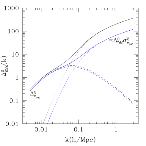
Figure 1.— The normalized KSZ cluster flux power spectra at $z=0$ (black line) and $z=1$ (blue) respectively. The dash lines are the contributions from the $vv$ term and the dot lines are the contributions from the $\delta v\delta v$ term. The solid line is the sum of them.

3. Noise estimation

We target at SPT to estimate the accuracy of $\Delta^{2}_{\rm KSZ}$ measurement. We assume that SPT will cover the $217$ Ghz range and $4400\ {\rm deg}^{2}$ with arc-minute resolution. We discuss the three dominant error sources, diffuse foregrounds and backgrounds (§3.1), sources associated with clusters (§3.2) and cosmic variance and shot noise (§3.3). We assume redshift bin size $\Delta z=0.2$ and $k$ bin size $\Delta k=0.5k$.

3.1. Diffuse foregrounds and backgrounds

The KSZ signal has typical $\Delta T_{\rm KSZ}\simeq 20\mu K\langle\tau\rangle/0.01$. Primary CMB, which is indistinguishable from the KSZ signal in frequency space, has intrinsic temperature fluctuation $\Delta T\sim 100\mu$K. The CIB has mean $T\sim 20\mu$K, if scaled to $217$ Ghz (Fixsen et al., 1998). A cluster KSZ filter can be applied to filter away the mean backgrounds while keeping the KSZ signal. This filter must strongly match the cluster KSZ profile while having zero integrated area. Since the angular size of clusters are generally several arc-minute, such filter naturally peaks at multipole $l$ around several thousands and thus naturally filters away the dominant CMB signal, which concentrates at $l\lesssim 1500$. For such filters, at $\sim 217$ Ghz, the galactic synchrotron, free-free foregrounds, the galactic dust emission, the radio background, the TSZ background are all negligible due to their frequency or scale dependence (see, e.g. Wright (1998); Bennett et al. (2003)). So we only discuss the contaminations of the primary CMB, CIB and background KSZ.

The optimal filter can be constructed from the intracluster gas profile inferred from the TSZ survey. For simplicity, we choose the electron density profile as $n_{e}(r)\propto(1+r^{2}/r^{2}_{c})^{-1}$ and a compensate Gaussian filter $W(l)=6(l/l_{f})^{2}\exp(-(l/l_{f})^{2})$. For these particular choices, filtered KSZ temperature, $\tilde{\Delta}T_{\rm KSZ}$, peaks at $l_{f}\sim 1.1/\theta_{c}\sim 3800(1^{{}^{\prime}}/\theta_{c})$, where $\theta_{c}$ is the angular core radius, and the peak value is $\tilde{\Delta}T_{\rm KSZ}\simeq\Delta T_{\rm KSZ}\simeq 9v_{100}[\langle\tau\rangle/0.01]\mu K$. For simplicity, we adopt this $l_{f}$ and $\theta_{c}=0.4{\rm Mpc/h}/\chi(z)$ to estimate the noise. Here, $\chi(z)$ is the comoving angular distance.

The correlations of filtered backgrounds (with zero mean flux), originating from both their intrinsic correlations and cluster clustering, are $\tilde{\xi}_{b}(r)\sim[\int_{m_{\rm low}}\Delta\Omega_{A}dn]^{2}[1+\langle b_{n}\rangle^{2}\xi_{\rm DM}(r)]\tilde{w}_{b}(\theta\sim r/\chi)$, where $\tilde{w}_{b}(\theta)$ is the corresponding (filtered) background angular correlation function.

The CMB contamination is sub-tractable and does not cause systematic error. The same cluster survey measures both $\int\Delta\Omega_{A}dn$ and $\langle b_{n}\rangle^{2}\xi_{\rm DM}$, while the CMB $C_{l}$ has been precisely measured by WMAP and can be precisely predicted by CMBFAST (Seljak & Zaldarriaga, 1996). Thus the CMB contamination $\tilde{\xi}_{\rm CMB}$ can be straightforwardly predicted and subtracted from the correlation estimator. Thus only the statistical errors caused by the CMB intrinsic fluctuation over cluster regions remains.

The CIB and KSZ contaminations are in principle sub-tractable, too. But since both the amplitude and shape of CIB and KSZ power spectra are highly uncertain, we do not attempt to subtract their contribution from the correlation estimator. The CIB power spectrum is $C_{l}^{\rm CIB}l^{2}/(2\pi)\simeq(4\mu{\rm K})^{2}(l/10^{3})^{0.7}$ (see, e.g. Zhang (2003)) and the kinetic SZ power spectrum is $C_{l}^{\rm back-KSZ}l^{2}/(2\pi)\simeq(2.7\mu{\rm K})^{2}$ (Zhang et al., 2004). The upper limit of the fractional systematic error they cause is

$$\eta \sim \frac{\left[\sum_{b={\rm CIB,KSZ}}C^{b}_{l}\frac{l^{2}}{2\pi}W^{2}(l,l_{f})\right]_{l\sim k\chi}}{[9(\langle\tau\rangle/0.01)\mu K]^{2}}\times$$ (6)

$$\frac{1+\langle b_{n}\rangle^{2}\Delta^{2}_{\rm DM}(k)}{\Delta^{2}_{v_{100}}(k)+\langle b_{n}\rangle^{2}\Delta^{2}_{\delta_{1}v_{1}\delta_{2}v_{2}}}\ ,$$

which is at most several percent at $k\lesssim 1h/$Mpc (Fig. 2).

Figure 2.— The dominant errors of the cluster KSZ power spectrum measurement. The solid lines are the errors caused by the cosmic variance and shot noise. The short dash lines are the systematic errors caused by the CIB and KSZ background. The long dash lines are the statistical errors caused by the primary CMB. The dot lines (which are visible only in the upper left panel) are the statistical errors caused by sources associated clusters. Systematic errors are sub-dominant at $k\lesssim 1h/$Mpc.

3.2. Sources associated with clusters

The map filter does not filter away the contaminations from sources associated with clusters. At $217$Ghz, the non-relativistic TSZ vanishes. But the relativistic correction of cluster TSZ effect shifts the cross over point slightly to higher frequency and thus in principle introduces a residual thermal SZ signal in $\sim 217$Ghz band. We assume an effective $\Delta T_{\rm TSZ}\sim 1\mu$K, or, $\sim 1\%$ of the TSZ at Rayleigh-Jeans regime. This gives a flux $S_{\rm res-SZ}\sim 540\ {\rm Jy}\ {\rm sr}^{-1}$. The flux of radio sources and IR sources associated with cluster is $\sim 10^{3}{\rm Jy}{\rm sr}^{-1}$ at $217$ Ghz (see, e.g. Aghanim et al. (2004)). By multi-frequency information and resolved source subtraction, one is likely able to subtract much of these contaminations. Rather conservatively, we assume that, at $\nu\sim 217$Ghz, the total flux contributed by those sources associated with clusters is less than $\sim 5\times 10^{3}{\rm Jy}{\rm sr}^{-1}$ at $z=0.5$ and scale it to other redshifts assuming no intrinsic luminosity evolution.

The mean flux of these sources is subtracted in our estimator (Eq. 2). Since the cluster thermal energy, IR and radio flux should be mainly determined by local processes, one can omit the possible large scale correlation of these quantities. Thus these sources do not cause systematic errors. But since $\langle\delta S_{\rm clst}^{2}\rangle\neq 0$, they do contribute to statistical errors. The fractional error they cause is

$$\eta \sim \frac{\langle\delta S_{\rm clst}^{2}\rangle}{S^{2}_{100}}\frac{\langle b_{n}\rangle^{2}\Delta^{2}_{\rm DM}2\pi[Vk^{2}\Delta k]^{-1/2}}{\Delta^{2}_{v_{100}}+\langle b_{n}\rangle^{2}\Delta^{2}_{\delta_{1}v_{1}\delta_{2}v_{2}}}$$ (7)

$$\lesssim 5\times 10^{-3}\frac{\langle\delta S_{\rm clst}^{2}\rangle}{S^{2}_{100}}z^{-1}\sqrt{\frac{\Delta z}{0.2}\frac{\Delta k/k}{0.5}}$$

Here, $V$ is the survey volume in the adopted redshift bin. It is reasonable to assume that $\langle\delta S^{2}_{\rm clst}\rangle^{1/2}\lesssim\langle S_{\rm clst}\rangle$. Thus the error caused by the sources associated with clusters is negligible at almost all scales and redshifts (Fig. 2)

3.3. Cosmic variance and shot noises

The signal intrinsic cosmic variance dominates at large scales. The amount of cluster is very limited, so the shot noise is large, even in the linear scales. The signal, the instrumental noise, the rms flux fluctuations of any contaminations projected onto or associated with clusters, such as primary CMB, IR and radio sources, all contribute to the shot noise, whose power spectrum is

$$\tilde{\Delta}^{2}_{\rm short}=\frac{k^{3}}{\bar{n}2\pi^{2}}\left(\tilde{\sigma}^{2}_{\rm CMB}+\tilde{\sigma}^{2}_{\rm CIB}+\tilde{\sigma}^{2}_{\rm KSZ}+\tilde{\sigma}^{2}_{\rm clst}+\cdots\right).$$ (8)

Here, $\bar{n}$ is the mean number density of observed clusters, which can be calculated given the halo mass function, the survey specification and the gas model. For simplicity, we assume $\bar{n}(z)=3\times 10^{-5}/(1+z)^{3}(h/{\rm Mpc})^{3}$. We only consider the listed 4 dominant sources, where $\tilde{\sigma}_{\rm CMB}\sim\tilde{\sigma}_{\rm CIB}\sim\tilde{\sigma}_{\rm KSZ}\sim 20\mu K$ and $\tilde{\sigma}_{\rm clst}\sim 5\mu K$. The beamed and filtered SPT instrumental noise has rms $\sim 1\mu$K and is thus negligible. For SPT, the error caused by the cosmic variance and shot noise ($\sim 10\%$) dominates over all other errors. The systematic errors are (almost) always sub-dominant. In this sense, our method is optimal to measure the cluster peculiar velocity. For a future all sky survey, total error can be reduced to several percent level.

Figure 3.— The time variation of $F_{1}(k=0.015h/$Mpc (solid lines) and $F_{2}(k=0.2h/{\rm Mpc},k_{o}=0.015h/{\rm Mpc}$ (dash lines) caused by wrong assumed cosmological parameters. Our fiducial model (black straight line) has $\Omega_{m}=0.3$ and $\Omega_{\Lambda}=0.7$. Blue, magenta, red and black curves correspond to $(\Omega_{m},\Omega_{\Lambda})=(1.0,0.0),(0.3,0.0),(0.5,0.5)$ and $(0.1,0.9)$, respectively.

4. Constraining cosmology

There are several ways to constrain cosmology from the KSZ observations, such as directly comparing the theoretical prediction of Eq. 2 with observations. Extra information contained in the correlation allows us to develop a least model dependent method. Defining $\eta(k)\equiv\Delta^{2}_{\rm KSZ}(k)/\Delta^{2}_{n}(k)$, utilizing the asymptotic behavior that $\eta(k\rightarrow 0)\rightarrow\langle S_{100}\rangle^{2}\beta^{2}E^{2}a^{2}/\langle b_{n}\rangle^{2}3k^{2}$ and $\eta(k\rightarrow\infty)\rightarrow\langle S_{100}\rangle^{2}\sigma_{v}^{2}$, we obtain two observables, $F_{1}(k)=\Delta^{2}_{\rm KSZ}(k)/\eta(k\rightarrow\infty)=\Delta^{2}_{v}(k)/\sigma^{2}_{v}$ in the regime where $k\lesssim 0.03h/{\rm Mpc}$, and $F_{2}(k,k_{o})=\Delta^{2}_{n}(k)/[\eta(k\rightarrow\infty)/\eta(k_{o}\rightarrow 0)]=\Delta^{2}_{\rm DM}(k)/[3\sigma^{2}_{v}k_{o}^{2}/\beta^{2}E^{2}a^{2}]$ in the linear regime where $k\lesssim 0.3h/$Mpc. $F_{1,2}$ should be $z$ independent. Redshift distortion and possible velocity bias do not change this characteristic behavior. But if the cosmology one choose is different from the real cosmology, $k_{w}/k_{r}$, the ratio of determined wave-vector $k_{w}$ with respect to the real $k_{r}$, will evolve with $z$. Because of the $k$ dependence of $F_{1}(k)$ and $F_{2}(k)$, a wrong cosmology will cause the determined $F_{1}$ and $F_{2}$ to vary with $z$. This behavior can be applied to constrain cosmology. One can show that $k_{\parallel,w}/k_{\parallel,r}=E_{w}(z)/E_{r}(z)=g_{\parallel}(z)$ and $k_{\perp,w}/k_{\perp,r}=\chi_{r}(z)/\chi_{w}(z)=g_{\perp}(z)$. Any measured quantity $\Psi(k)$ are then the corresponding quantity averaged over all configurations, namely, $\langle\Psi(k,u)\rangle\equiv\int_{-1}^{1}\Psi\left[k\sqrt{u^{2}/g_{\parallel}^{2}+(1-u^{2})/g^{2}_{\perp}}\right]du/2$. We obtain

$$\frac{F_{1,w}(z)}{F_{1,w}(z_{0})}|_{k} = \frac{\langle\Delta^{2}_{v}(k,u)\rangle}{\Delta^{2}_{v}(k)}$$ (9)

$$\frac{F_{2,w}(z)}{F_{2,w}(z_{0})}|_{k,k_{o}} = \frac{\langle\Delta^{2}_{\rm DM}(k,u)\rangle}{\Delta^{2}_{\rm DM}(k)}\frac{\Delta^{2}_{\rm DM}(k_{o})}{\langle\Delta^{2}_{\rm DM}(k_{o},u)\rangle}\frac{\langle\Delta^{2}_{v}(k_{o},u)\rangle}{\Delta^{2}_{v}(k_{o})}\ .$$

Fig. 3 shows the $z$ dependence of $F_{1,2}(z)$ for various assumed cosmologies. This variation can reach $\sim 20\%$ and thus should be detected by SPT. A future all sky survey would measure this variation to better than $\sim 5\%$ accuracy and should provide a tight and independent cosmology check. The nonlinearity correction, the parallel line of sight approximation, etc. may cause non-negligible systematics. But these effects are straightforward to predict and correct, so we postpone the discussion of these effects in this paper.

5. Conclusion

We present a new method to measure the peculiar velocity power spectrum $\Delta^{2}_{v}$ by directly correlating the KSZ flux. The cluster peculiar velocity signal is amplified in the direct correlation. Many systematics involved in the usual $v_{p}$ inversion disappear and the majority of remaining systematics can be easily subtracted. The correlation method is optimal to measure $\Delta^{2}_{v}$, in the sense that statistical error, dominates over systematics at almost all $k$ and $z$ range. We estimate that SPT can measure $\Delta^{2}_{v}$ to $\sim 10\%$ accuracy and a future all sky survey can improve this measurement by a factor of several. The KSZ flux correlation contains extra information on the velocity dispersion. This extra information helps to construct two independent observables as indicators of Hubble constant and comoving angular distance, with only minimal amount of assumptions. These observables should put independent constraints on cosmology.

Acknowledgments: P.J. Zhang and A. Stebbins are supported by the DOE and the NASA grant NAG 5-10842 at Fermilab.

References

• Aghanim et al. (2001) Aghanim, N., Gorski, K.M., & Puget, J.-L., 2001, A&A, 374
• Aghanim et al. (2004) Aghanim, N., Hansen, S., & Lagache, G., 2004, astro-ph/0402571
• Atrio-Barandela et al. (2004) Atrio-Barandela, F., Kashlinsky, A., & Mucket, J.P., 2004, ApJ, 601, L111
• Bardeen et al. (1986) Bardeen, J.M., et al., 1986, ApJ, 304, 15
• Bennett et al. (2003) Bennett, C.L., et al. 2003, ApJs, 148, 97
• Davis & Peebles (1983) Davis, M.Β & Peebles, P.Β J.Β E.Β 1983, ApJ, 267, 465
• Diaferio et al. (2004) Diaferio, A., et al. 2004, astro-ph/0405365
• Feldman et al. (2003) Feldman, H., et al.Β 2003, ApJ, 596, L131
• Fixsen et al. (1998) Fixsen, D.J., et al., 1998, ApJ, 508, 123
• Haehnelt & Tegmark (1996) Haehnelt, M.G., & Tegmark, M., 1996, MNRAS, 279, 545
• Hansen et al. (2002) Hansen, S.H., Pastor, S., & Semikoz, D.V., 2002, ApJ, 573, L69
• Holder (2004) Holder, G., 2004, ApJ, 602, 18
• Hu & Lou (2004) Hu, J., & Lou, Y.Q., 2004, ApJ, 606, L1
• Kaiser (1987) Kaiser, N.Β 1987, MNRAS, 227, 1
• Kashlinsky & Atrio-Barandela (2000) Kashlinsky, A., & Atrio-Barandela, 2000, ApJ, 536, L67
• Knox et al. (2003) Knox, L., Holder, G., & Church, S., 2003, astro-ph/0309643
• Seljak & Zaldarriaga (1996) Seljak, U., & Zaldarriaga, M., 1996, ApJ, 469, 437
• Wright (1998) Wright,E., 1998, ApJ, 496, 1
• Zhang (2003) Zhang,P., 2003, astro-ph/0307440
• Zhang et al. (2004) Zhang, P., Pen, U.L., & Trac, H., 2004, MNRAS, 347, 1224