The CIDA Variability Survey of Orion OB1. I: the low-mass population of Ori OB 1a and 1b

Abstract

We present results of a large scale, multi-epoch optical survey of the Ori OB1 association, carried out with the QuEST camera at the Venezuela National Astronomical Observatory. We identify for the first time the widely spread low-mass, young population in the Orion OB1a and OB1b sub-associations. Candidate members were picked up by their variability in the $V$-band and position in color-magnitude diagrams. We obtained spectra to confirm membership. In a region spanning $\rm\sim 68\Box^{\circ}$ we found 197 new young stars; of these, 56 are located in the Ori OB1a subassociation and 142 in Ori OB1b. The spatial distribution of the the low mass young stars is spatially coincident with that of the high mass members, but suggests a much sharper edge to the association. Comparison with the spatial extent of molecular gas and extinction maps indicates that the subassociation Ori 1b is concentrated within a ring-like structure of radius $\sim$ 2${}^{\circ}(\sim$ 15 pc at 440 pc), centered roughly on the star $\epsilon$ Ori in the Orion belt. The ring is apparent in ¹³CO and corresponds to a region with an extinction $A_{V}\geq 1$. The stars exhibiting strong H$\alpha$ emission, an indicator of active accretion, are found along this ring, while the center is populated with weak H$\alpha$ emitting stars. In contrast, Ori OB1a is located in a region devoid of gas and dust. We identify a grouping of stars within a $\rm\sim 3\>deg^{2}$ area located in 1a, roughly clustered around the B2 star 25 Ori. The Herbig Ae/Be star V346 Ori is also associated with this grouping, which could be an older analog of $\sigma$ Ori. Using using several sets of evolutionary tracks we find an age of 7 - 10 Myr for Ori 1a and of $\sim 4-6$ Myr for Ori OB1b, consistent with previous estimates from OB stars. Indicators such as the equivalent width of H$\alpha$ and near-IR excesses show that the number of accreting low-mass stars decreases sharply between Ori 1b and Ori 1a. These results indicate that while a substantial fraction of accreting disks remain at ages $\sim 5$ Myr, inner disks are essentially dissipated by 10 Myr.

1 Introduction

The Orion OB1 Association, located at roughly 400 pc (see review by Genzel & Stutzki 1989) and spanning over $\rm 200\>deg^{2}$ on the sky, is one of the largest and nearest regions with active star formation. With a wide range of ages and environmental conditions, Orion is an ideal laboratory for investigating fundamental questions related to the birth of stars and planetary systems. Blaauw (1964) identified four major subgroups which differ in age and their content of gas and dust: Ori OB1a, 1b (that roughly encompasses the belt stars $\delta$, $\epsilon$ and $\zeta$ Ori), 1c and 1d (where the Orion Nebula Cluster [ONC] is located). Within this vast region there are extremely young groupings of stars still embedded in their parent clouds, such as NGC 2068, 2071, 2023 and 2024 in the Orion B molecular cloud, observed mostly at IR and sub-mm wavelengths (Dahari & Lada 1999; Haisch et al. 2001; Motte et al. 2001); the young, dense, and partially embedded ONC (Herbig & Terndrup, 1986; Ali & Depoy, 1995; Hillenbrand, 1997, hereafter H97); clusterings of intermediate age ($\sim 3-5$ Myr) stars including the $\sigma$ Ori (Garrison, 1967; Walter et al., 1997) and $\lambda$ Ori groups (Murdin & Penston, 1977; Dolan & Mathieu, 1999, 2001, 2002) and older populations like the $\sim 10$ Myr old OB1a sub-association, located in an area essentially devoid of gas and dust.

While the earliest stages of stellar evolution must be probed with infrared and radio techniques, many fundamental questions including lifetimes of molecular clouds, cluster dispersal, protoplanetary disk evolution and triggered star formation, can only be addressed by optical surveys of older populations with ages $\sim$ 3-20 Myr. To make progress on these issues, wide-field studies of stellar populations in and near star-forming regions are required. In the past, studies of OB associations have been used to investigate sequential star formation and triggering on large scales (e.g., Blaauw 1991 and references therein). However, OB stars are formed essentially on the main sequence (e.g. Palla & Stahler 1992, 1993) and evolve off the main sequence on timescales of order 10 Myr (depending upon mass and amount of convective overshoot); thus, they are not useful tracers of star-forming histories on timescales of 1-3 Myr. Moreover, we cannot investigate cluster structure and dispersal or disk evolution without studying low-mass stars. Wide-field studies of the low mass populations have been carried for some portions of the Upper Scorpius OB association (Preibisch & Zinnecker, 1999; Preibisch et al., 2002). In Orion, many young individual clusters have been studied at both optical and infrared wavelengths (e.g. Lada 1992; Prosser et al. 1994; Hillenbrand 1997; Stassun et al. 1999), but these only represent the highest-density, and often youngest, regions. Little is known about the more widely spread low mass stellar population in these OB associations.

A few large scale surveys have tried to map the widely distributed low-mass pre-main sequence population in Orion. The Kiso objective-prism H$\alpha$ survey (Wiramihardja et al., 1989, 1991, 1993; Kogure et al., 1989; Nakano et al., 1995), covered 225$\Box^{\circ}$ around the clouds but was biased towards the strongest H$\alpha$ emitting stars. The ROSAT All-Sky Survey (Alcalá et al., 1996) detected many X-ray strong young stars widely distributed across Orion; however, this selection was strongly affected by older foreground field stars unrelated to the young population of Orion (Briceño et al., 1997) and because of its shallow limit it did not reach the fainter K and M stars. (Walter, Wolk & Sherry, 1998) carried out a detailed photometric and spectroscopic study of the region around the O9.5 type star $\sigma$ Ori, belonging to 1b, and found a large concentration of pre-main sequence low mass stars down to V $\sim$ 19. Similar high densities of young low mass stars have been found in other selected small regions in 1a and 1b by Sherry et al. (1999) and Sherry (2003), indicating that many low mass stars remain undiscovered.

Until recently, it was not possible to conduct unbiased, large-scale optical surveys but technological advances have now made it possible, building on the availability of cameras with multiple CCDs and multiobject spectrographs on telescopes with wide fields of view. One such survey is the optical variability study we have conducted over $\rm\sim 173\>deg^{2}$ in the Orion OB1 association with the purpose of finding, mapping, and studying large numbers of widely-dispersed, low mass ($\lesssim 1M_{\sun}$) stars with ages from 1 to $\sim$ 20 Myr.

Optical photometric variability is one of the defining characteristics of pre-main sequence stars (Joy, 1945; Herbig, 1962). However, due to limitations in the size of CCD detectors, past work on photometric variability of young stars have concentrated on follow up studies of selected samples, that had been identified as pre-main sequence objects by some other means. Only very recently has the potential of variability as a technique to pick out young stars amongst the field population started to be realized (Briceño et al., 2001; Lamm et al., 2004).

In this contribution we present results from our variability survey in an area of nearly $\rm 68\>deg^{2}$, that includes the Ori OB1b sub-association, a large fraction of Ori OB1a, and part of the Orion B molecular cloud (Maddalena et al., 1987), with the young clusters NGC 2023, 2024, 2068 and 2071. In §2 we describe the optical variability survey and follow up spectroscopy. In §3 we describe our results, and in §4 we present a discussion and conclusions.

2 Observations and Data Reduction

2.1 The QuEST Camera

The multi-band, multi-epoch photometric survey was carried out using an $8000\times 8000$ CCD Mosaic Camera built by the QuEST collaboration and installed on the 1m (clear aperture) Schmidt telescope at the Llano del Hato National Astronomical Observatory, located at an elevation of 3610 m in the Venezuelan Andes, close to the equator ($8^{\circ}47^{\prime}$ N) and under dark skies. The 16 $2048\times 2048$ Loral CCD devices are set in a 4x4 array covering most of the focal plane of the Schmidt telescope. The chips are front illuminated with a pixel size of $15\mu$m, which corresponds to a scale of 1.02” per pixel. Because of the gaps between rows of CCDs in the east-west direction, the effective field of view is $\rm 5.4deg^{2}$ (see Baltay et al. 2002 for a detailed description of the instrument).

The camera has been designed for observing in drift-scan mode: the telescope is fixed and the CCDs are read out E-W at the sidereal rate as stars drift across the device. This procedure results in the generation of a continuous strip (or “scan”) of the sky, $2.3^{\circ}$ wide; the sky can be surveyed at a rate of $34.5\Box^{o}/hr$. In addition to its high efficiency for covering large areas in a short time, drift-scanning offers other significant advantages: the telescope does not have to be moved so there is no time lost for reading out the CCDs. Also, flat-fielding errors are minimized, since each stellar image is obtained by averaging over many pixels as it travels over the CCD, and astrometric precision is enhanced because the zenith angle is constant throughout. One of the limitations of drift-scanning is that the sky motion is only parallel on the equator and the rate of drift on the focal plane is a function of the declination. To address this effect, each row of CCDs is mounted on a separate ”finger” which pivots at one end, allowing the row to be independently aligned perpendicular to the star paths by moving an eccentric cam at the opposite end. The chips are clocked out at separate rates to compensate for the change in sidereal rate as a function of declination; even so, the size of the devices and the image scale limit the declination range available for drift-scanning. To minimize image smearing to $\leq 0.5$ pixel, drift-scanning is restricted to $-6^{\circ}\leq\delta\leq+6^{\circ}$. The drift-scan mode allows to obtain quasi-simultaneous multi-band photometry since each column of chips, oriented N-S, can be fitted with separate filters; stars will successively cross over 4 chips in a column each with its own filter . Several filters are available, including BVRI and $\rm H\alpha$. The exposure time (hence the limiting magnitude) are set by the time a star needs to cross a single chip (140 sec at $\delta=0^{\circ}$). Deeper images can be obtained by combining several scans. This combination of exposure time with the typical seeing at the site (see below) result in a $10\sigma$ limiting magnitude of $\sim 19.5$ in the V-band. Saturation occurs at $V=13.0-14.5$ depending on the CCD, since they have differing well depths. The data acquisition system is described in Sabbey et al. (1998).

2.2 The Optical Variability Survey

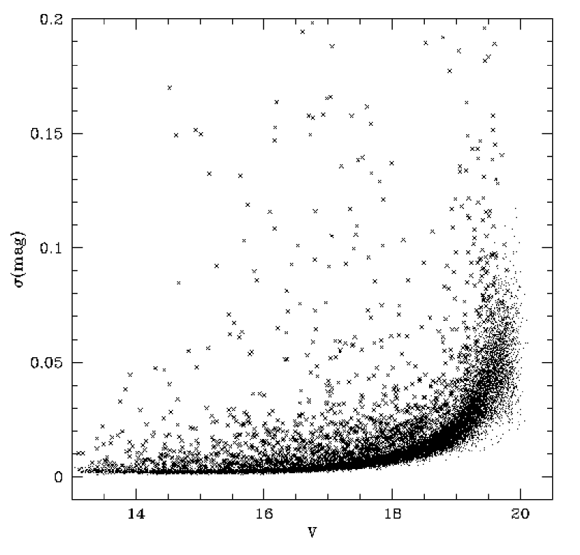
Figure 1: The $1\sigma$ dispersion of up to 32 $V$-band magnitude measurements for $\sim 30000$ stars in a $\rm 5.3\>deg^{2}$ portion of the Orion variability survey. Crosses indicate the stars selected as variable by the $\chi^{2}$ test.

The location of the telescope, together with the advantages of the drift-scan technique make this an ideal survey instrument for large scale studies of regions close to the celestial equator like Orion. Our photometric survey spans the region from 5h - 6h in RA and $\rm DEC=-6^{\circ}to+6^{\circ}$, shown in Figure 1 of Briceño et al. (2001). We covered this large portion of the sky in 6 strips at constant declination, centered at $\rm DEC=-5^{\circ},-3^{\circ},-1^{\circ},+1^{\circ},+3^{\circ}and+5^{\circ}$, for a total area of $\rm\sim 173\>deg^{2}$ (because of the $\sim 50\arcsec$ gaps between CCDs in DEC, we lose about $\rm 1.1\>deg^{2}$ per scan). Here we present results for two strips at $\rm DEC=-1^{\circ}\>and\>+1^{\circ}$, encompassing an area of nearly $\rm 68\>deg^{2}$, and a spanning the range $l\rm\sim 200^{\circ}\>to\>\sim 210^{\circ}$ and $\rm|b|=-10^{\circ}\>to\>-22^{\circ}$. This part of Orion includes the region around the belt stars $\delta$, $\epsilon$, and $\zeta$, that constitutes the OB1b sub-association Warren & Hesser (1977, 1978, hereafter WH) the region north and west of it, the OB1a sub-association, and part of the Orion B molecular cloud (Maddalena et al., 1987), with the young clusters NGC 2023, 2024, 2068 and 2071.

Our scans start on average a little before $\rm RA=5^{h}$ and end a little beyond $\rm RA=6^{h}$, in order to have complete coverage in all filters in the range $\rm RA=5^{h}-6^{h}$. Some of our observations were shared with other projects, therefore a number of our scans, especially at $\rm DEC=-1^{\circ}$, start at RA $\rm\sim 3-4^{h}$. In practice, the start time and length of each drift scan was determined by the sky conditions; some scans had to be cut short of $\rm RA=\sim 6^{h}$. The temporal spacing between observations was mostly determined by weather and scheduling constraints because of other ongoing projects with the instrument. We obtained 23 scans at $\rm DEC=-1^{\circ}$ during 18 nights from December 1998 through January and February 1999 and then from late 1999 through early 2000; the 33 scans at $\rm DEC=+1^{\circ}$, collected over 17 nights, are more sparsely distributed in time, starting in Dec. 1999, continuing in October 2002, January and February 2003, with the final data obtained in October 2003. The observation log is shown in Table 1. The general observational strategy was to observe as close to the meridian as possible with a maximum hour angle of $\rm 2\fh 5$; because of this and the equatorial location of Llano del Hato, the airmass for most of our observations is $\lesssim 1.3$. The typical seeing during our observations ranged from $1.8\arcsec$ to $\sim 2.5\arcsec$; however, due to the expected degradation introduced by drift-scanning (Gibson & Hickson, 1992) combined with the pixel size, most scans have images with FWHM $\sim 2.5-3\arcsec$. Thus, with a pixel scale of $1\farcs 02$ the point spread function is well sampled.

2.3 Data Processing and Variable Star Identification

In order to effectively process the approximately 30 Gb/night of raw data produced by this instrument, QuEST developed its own software. The whole process is completely automated with minimum interaction from the user. The QuEST offline software performs the basic reduction: overscan subtraction and flat-fielding (one-dimensional flats are used to correct the response variations along the N-S direction); object detection and seeing determination (by measuring an average FWHM for $\sim 10^{2}-10^{3}$ of stars in each frame); determines the positional offsets between CCDs (recognizes a single star in all 4 fingers - rows); performs aperture photometry with an aperture radius based on the FWHM of the particular frame (several apertures are used: 1$\times$FWHM, 2$\times$FWHM, etc.); finally, Astrometry is done by matching the objects with the USN-A2.0 catalog (Monet et al., 1998). Positions are internally accurate to $\pm 0.2\arcsec$. Each catalog for every drift scan is stored in binary format and contains, among others, positions J2000.0, instrumental magnitudes in 4 bands, errors, fluxes within several apertures, flags (bad columns, edges, etc.). A detailed description of the data pipeline is given in Rengstorf et al. (2004).

We have used differential photometry to identify variable stars among this large number of objects. Our main interest is picking out candidate pre-main sequence stars among the general field population. Low-mass ($\rm M\lesssim 2\>M_{\sun}$) young stars (T Tauri stars, hereafter TTS) are known to vary on time scales from hours to weeks, with variations of up to a few magnitudes. Usually the variations are larger in the $V$-band than in the $I$-band. This variability can be irregular, thought to originate in flare-like activity or in non-steady accretion for the strong H$\alpha$ emitting objects (Classical T Tauri stars, CTTS); the periodic variations, seen mostly in weak H$\alpha$ emitting TTS (WTTS), are proposed to be the result of rotational modulation by hot or cool stellar spots in the star’s surface (Herbst et al., 1994) Therefore, our choice of the $V$ filter allows us to sample a wavelength range were TTS are expected to vary the most. Also, because we are not aiming at obtaining light curves or deriving periods for our stars, our irregular temporal sampling is not a major limitation, in fact, since our data spans time scales from hours (in a few cases), to days, months and years, we expect to detect most of the TTS within our survey area and down to our sensitivity limits.

In order to derive the relative photometry we first chose as reference catalogs those corresponding to scans obtained during clear nights, which showed a stable behavior of the sky background as a function of RA as measured from the average value for the ensemble photometry of thousands of stars in each frame. For the DEC=$-1^{\circ}$ strip we used observation No. 512 from January 06, 1999, and observation No. 502 from December 26, 1999 for DEC=$+1^{\circ}$. After doing a positional matching, within a $2\arcsec$ search radius, of all stars in each reference scan with respect to the other scans, we obtained a final combined catalog for the DEC=$-1^{\circ}$ and $+1^{\circ}$ strips containing 340,532 objects, which had a minimum of three good measurements. This master catalog incorporated data from 21 out of the 23 scans at $\rm DEC=-1^{\circ}$ and 31 of the 33 scans at $\rm DEC=+1^{\circ}$. Some scans had to be discarded because of excessive cloud cover during the observation.

The instrumental magnitudes were normalized to each reference scan in order to remove variable atmospheric extinction due to differences in air mass and sky transparency. This normalization to reference magnitudes was done in bins of $0.25^{\circ}$ of right ascension, equivalent to $\sim 1$ minute of time in drift-scan mode. Then we calculated the magnitude differences between each scan and the reference scan for all stars in each bin of right ascension, and an ensemble clipped mean was produced. Since each bin typically contains several hundred stars, especially at the relatively low galactic latitude of our survey area, this procedure gives a robust estimate of the zero-point difference between each scan and the reference one. With this approach, variable sky conditions like a passing cloud causing an extinction of up to 1 magnitude can be corrected, as shown in Figure 3 of Vivas et al. (2004), where more details of this method are provided.

Since a large number of stars have been measured, the random errors of the differential magnitudes are well determined. These amount to $\sim 0.005$ magnitudes for $V\leq 17$ and increase to $\sim 0.08$ mag at $V\sim 19.7$ as photon statistics dominate the noise. Because of the larger errors when progressing toward the limiting magnitude of our observations, fainter variables are biased toward larger values of $\rm\Delta V$. In Figure 1 we show the dispersion in the normalized instrumental $V$-band magnitudes for a subsample of the data corresponding to an area of $\rm 5.2\>deg^{2}$ containing $\sim 30,000$ stars. Each point represents the statistics of up to 32 measurements. Objects detected as variables are indicated with an ”x” mark. Most objects are non-variable and populate the curved region; points above the curve are likely variable stars.

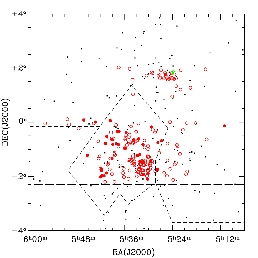
Figure 5: Spatial distribution of the young stars found in the Orion survey: CTTS (large solid circles), WTTS (large open circles). The approximate limits of the scans are indicated by long dashed. The small dashes line marks the boundaries of Ori 1a, 1b, and 1c as defined by Warren & Hesser (1977). The small squares show the positions of the OBA stars in the associations (Hernández et al. 2004), selected from the Hipparcos catalog with proper motions criteria from from Brown et al. (1994). The asterisk marks the Herbig Ae/Be star V346 Ori, located in the clump of stars in Ori OB1a.

Following Vivas et al. (2004) we applied a $\chi^{2}$ test on the normalized magnitudes to select variable stars, which is appropriate because non-variable stars follow a Gaussian distribution of errors (Figure 5 in Vivas et al., 2004) If the probability that the dispersion is due to random errors is very low ($\leq 0.01$), the object is flagged as variable. Before running the $\chi^{2}$ test we eliminated measurements that are potentially affected by cosmic rays, by deleting points that were more than $4\sigma$ away from the mean magnitude for that particular object. We flagged all objects with a 99% confidence level of being variable [$\rm P(\chi^{2})\leq 0.01$]. This confidence level sets the minimum $\Delta{\rm mag}$ that we can detect as a function of magnitude: 0.06 for $V=15$, 0.09 for $V=17$ and 0.30 for $V=19$. This means that for fainter stars we detect only those which vary the most. We cannot decrease the confidence level very much without increasing the contamination from non-variable stars to unacceptable levels because we are studying hundreds of thousands of stars. Following this scheme we detected 20729 variables in the $\rm DEC=-1^{\circ}$ and $\rm DEC=+1^{\circ}$ strips, a $\sim 6$% fraction of variable stars. The selection criterion we used still allows $\sim 3400$ possible spurious variables. The fraction of variables we find is larger than that found by other variability surveys, e.g. 0.4% in the All Sky Automated Survey (Pojmánski, 2003), and 0.8% in the ROTSE variability survey (Akerlof et al., 2000). However, the fraction of false variables in our data may be quite higher than the number expected from the confidence level of the $\chi^{2}$ test alone. This could be the result of close neighbors and blends, especially at the galactic latitude of Orion. We did not attempt to identify these false variables because our selection criteria include additional constraints, particularly spectroscopy, that will further reject contaminants. At this point we proceeded to plot the variables in color-magnitude diagrams to select pre-main sequence candidates.

For the calibration of the photometry we used the Smithsonian Astrophysical Observatory (SAO) 1.2m telescope equipped with the 4SHOOTER CCD Mosaic Camera (Caldwell & Falco, 1993) at Mt. Hopkins, Arizona, during the nights of Dec. 3 and 4, 2002. The 4SHOOTER is an array of four CCDs, covering a square of $\sim$25 arcminutes side, with the four chips of approximately 12 arcminutes side. We used a binning of $2\times 2$ yielding a plate scale of 0.66 ″/pix. We obtained $V$ and Cousin $I$-band images of selected fields at RA=5h-6h, with declinations such that they would fall on parts of the sky overlapping each of the four columns in our QuEST Camera scans. Throughout each night we observed the Landolt (1992) standard fields PG0231+051, SA 92 and SA 98 at airmasses. 1-1.5. We centered all our target fields on chip 3, the detector with best cosmetics. Raw images were bias-subtracted and flattened (with dome flats) using standard IRAF routines. We then performed aperture photometry on all our frames. Typically we had 12-20 standard stars per night. Our photometric solution was derived with a rms of 0.02 mags for $V$ and 0.03 mags for $I_{C}$, In each of the secondary standard fields we selected stars in the range $V=15-18$, much fainter than our saturation limit, and bright enough to yield a good SNR. Positions within 0.5″were obtained using the CM1 program Stock & Abad (1988) to produce a plate solution for each frame, after comparing with $\sim 6$ reference stars from the Guide Star Catalog. This accuracy is enough for positional matching with our QuEST Camera catalog. Finally, we kept only those stars with more than 7 measurements and not flagged as variable by our variability selection scheme (see below). Our final list contains 390 secondary standards, a robust set of comparison stars which we used to calibrate the normalized magnitudes computed by our variability programs from the QuEST Camera scans.

2.4 Selection of candidate pre-main sequence stars

Traditional multicolor photometric surveys for pre-main sequence stars have relied mainly on color-magnitude and color-color diagrams to select candidate young stars. This approach has been feasible for previous studies that dealt with regions spanning small areas. However, because of the large number of potential pre-main sequence stars in our survey, and the contamination by large numbers of field stars, this selection method is too inefficient. We therefore use variability to select candidate association members.

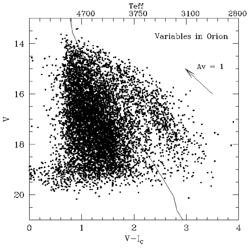
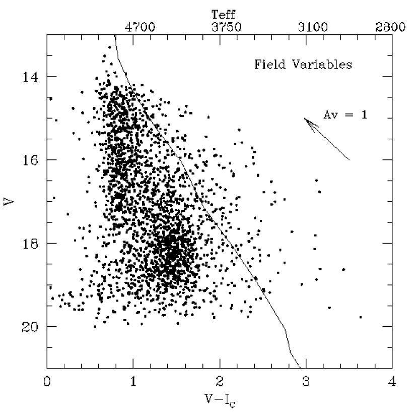
Figure 2: Color-magnitude diagrams for stars selected as variable. Left panel: all variables detected in the $\rm DEC=-1^{\circ}$ strip with $\rm RA>5^{h}$. Right panel: control field off Orion; stars in the same strip and with $\rm RA=4^{h}48^{m}-5^{h}00^{m}$.

In Figure 2 of Briceño et al. (2001) we showed that even in a modest region of $\rm\sim 10\>deg^{2}$ towards Ori OB1b there can be of the order of 4000 objects above the ZAMS down to $V\sim 19.5$; after object lists are filtered by our variability criterion only $\lesssim 10$% remain above the ZAMS. Moreover, selection of variable stars above the ZAMS clearly picks a significant fraction of the young stars in Orion, as shown in Figure 2, where we compare color-magnitude diagrams for a region in OB1b ($l\sim 203^{o}$, $b\sim-18^{o}$) and a control field ($l\sim 195^{o}$, $b\sim-31^{o}$), located well off Orion; the Orion field exhibits an excess of objects above the ZAMS not present in the control field, even after taking into account that the Orion region has a higher density of stars because it is closer to the galactic plane. In the Orion field the fraction of variables above the ZAMS is 19% compared to 10% in the control field, a factor of $\sim 2$ over density. However, the densest concentration of points in the color-magnitude diagram for the Orion field occurs at roughly 1 magnitude above the ZAMS. If we compare this locus in both panels of Figure 2, the fraction of variables above the ZAMS in the Orion field is a factor of 3 larger than in the control field.

We tested the reliability of the technique by recovering as variables the 15 out of 19 previously known pre-main sequence objects (Herbig & Bell, 1988) among the stars selected as variable above the ZAMS (see §3.1). We also used our results to estimate the minimum number of observations required to detect a star as variable. We took the data for five of the Herbig & Bell (1988) stars in our sample and at random took out data points from each star’s light curve, running the $\chi^{2}$ test each time. Accounting for points rejected due to objects falling on bad columns, we find that a minimum of 5 observations are needed to obtain a reliable detection.

The number of variables in the left panel of Figure 2 decreases with increasing V and V-I. This is a result both of the decreased sensitivity in the V band for redder objects, and of our selection criteria for variables. We selected a total of 3744 objects flagged as variable down to our limit of V$\sim 19.7$, and located above the ZAMS (Baraffe et al., 1998) in the $V$ vs. $V-I_{C}$ diagram. Within this sample we selected objects located above the 10 Myr isochrone as our highest priority candidates (we excluded from this list the previously known T Tauri stars in the region). We established a magnitude cutoff at $V=16$. Brighter than this magnitude we included all variables above the ZAMS; here we discuss follow up spectroscopy for 1083 of them. In the magnitude range $\rm V=16-18.5$ we assigned the highest priority to all variables above the ZAMS, we then added a number of non-variable stars in the same region of the color-magnitude diagram. We adopted this strategy in order to circumvent the problem of missing a significant fraction of low-mass, young stars at fainter magnitudes. A total of 320 of the $\rm V=16-18.5$ objects are discussed in this work.

Summarizing, our selection scheme of candidate Orion members started with 20729 objects flagged as variables among 340532 detections. We then selected 3744 of the variables that were located above the ZAMS in the color-magnitude diagram. Finally, we obtained spectra for a subset of those. Here we discuss follow up spectroscopy for 1403 objects.

2.5 Spectroscopy

Follow up spectra are necessary to provide confirmation of pre-main sequence low-mass stars. Optical spectra of TTS are characterized by emission in the Balmer lines, particularly H$\alpha$, other lines like Ca I H & K, as well as the presence of the Li I$\lambda 6707$Å line in absorption. Weak H$\alpha$ emission lines and Li I can be reliably measured in low resolution spectra, which are easiest to obtain at many moderate aperture telescopes (Briceño et al., 1998, 2001). Also, low resolution spectra usually span a large wavelength range, which provides a reasonable number of features (like TiO absorption bands in K through M type stars) for reliable spectral typing, from which $\rm T_{eff}$ can be derived.

Optical spectra were obtained in queue mode for 1083 of the brighter candidates ($V<16$) during the period January 1999 through January 2002, using the 1.5 meter telescope of the Whipple Observatory with the FAST Spectrograph (Fabricant et al., 1998), equipped with the Loral $512\times 2688$ CCD. The spectrograph was set up in the standard configuration used for “FAST COMBO” projects, a 300 groove $mm^{-1}$ grating and a 3” wide slit. This combination offers 3400 Å of spectral coverage centered at 5500 Å, with a resolution of 6 Å. The spectra were reduced at the CfA using software developed specifically for FAST COMBO observations. All individual spectra were wavelength calibrated using standard IRAF routines The effective exposure times ranged from 60 s for the $V\sim 13$ stars to $\sim 1500$ seconds for objects with $V\sim 16$. The signal-to-noise ratio (SNR) of our spectra are typically $\gtrsim 25$ at H$\alpha$, sufficient for detecting equivalent widths down to a few tenths of Å at our spectral resolution. In Figure 3 we show examples of typical FAST spectra.

We obtained optical spectra for a sample of faint targets ($V16-18.5$) using the Hydra multi-object spectrograph installed on the KPNO 3.5m WIYN telescope, during the nights of November 26 and 27, 2000 with clear weather. We discuss here spectroscopy of 320 candidate objects distributed in 5 fields spanning an area of $\rm\sim 4\Box^{\circ}$; details are shown in Table 2 (Note that Field 2b is the same region as Field 2a but with fibers located on different sets of objects). We used the Blue Channel fibers ($3\farcs 1$ diameter), the Simmons Camera with the T2KC CCD, the 400@4.2 grating, and G3_GG-375 bench filter, yielding a wavelength range $\sim 4000-7000$Å with a resolution of 7.1Å. All fields were observed with airmasses=1.0-1.5, and exposure times for individual exposures were 1800 s. When weather allowed we obtained two or three exposures per field. Comparison CuAr lamps were obtained between each target field.

Following the strategy outlined in §2.4, in each Hydra field we first assigned fibers to all variables above the ZAMS and with V$16-18.5$, then filled the remaining fibers with non-variable objects located in the pre-main sequence region of the $V$ vs. $V-I_{C}$ diagram and with V$16-18.5$. When possible we also assigned fibers to bright $V<16$ TTS confirmed from FAST spectra. Typically we assigned 10-12 fibers to empty sky positions and 5-6 fibers to guide stars. We used standard IRAF routines to remove the bias level from the two dimensional Hydra images. Then the dohydra package was used to extract individual spectra, derive the wavelength calibration, and do the sky background subtraction. Since the majority of our fields are located in regions with little nebulosity, background subtraction was in general easily accomplished.

3 Results

3.1 New members

Table 3 lists 197 new members of Ori OB1 found in the survey so far. (57 in Ori OB 1a, 138 in 1b, and 6 in 1c.) The first column of the table gives the CIDA Variability Survey of Orion (CVSO) running number. Column 2 gives the name of the counterpart in the All Sky release of the 2MASS catalog and columns 4 and 5 give the 2MASS positions.

The association between QuEST and 2MASS was made as follows. Positions obtained with the QuEST camera are internally accurate to $0\farcs 2$. We used a 5″search radius to match our positions for 165,530 objects in the $\rm DEC=-1^{\circ}$ strip with 2MASS; we found a median offset of $0\farcs 67\pm 0\farcs 22$. However, because the object surface density increases towards the galactic plane, confusion starts to be an issue at $\rm RA\gtrsim 5^{h}30^{m}$; the automated pipeline is not designed to deal with objects which are separated less than $\rm\lesssim 2$ FWHM. The result is that candidate lists have to be collated manually for blends. Thus, we inspected visually the DSS red plate images for each selected candidate. With a plate scale of $0\farcs 5$ the DSS can resolve close pairs better than our QuEST camera images. Still, some close pairs were observed spectroscopically (see below). Once we determined the new members, we searched in the 2MASS catalog for all sources within 10” from the QuEST position. We calculated the expected J magnitude of the counterpart, from V and extinction estimated from V-I using the interstellar reddening law (§3.4). For 191 stars, we found only one source within this search radius with J within 0.5 magnitudes of the expected J. However, for 6 stars (2, 34, 59, 114, 170, and 186 in Table 3), we found two 2MASS sources with comparable J magnitudes within the search radius. These stars were not resolved in the QuEST photometry, shown in columns 5 and 6 of Table 3, so we list the table the two possible counterparts and note that the optical photometry corresponds to the blend of both sources.

In columns 10 and 11 of Table 3 we show the equivalent width of H$\alpha$ and Li 6707. In column 12, we show the classification of the star according to the equivalent width of H$\alpha$. We follow White & Basri (2003) and use a limiting value between strong emission or Classical T Tauri stars (CTTS, ”C” in Table 3) and weak T Tauri stars (WTTS, ”W” in Table 3) which depends on spectral type: 3 Å if the spectral type is K5 or earlier, 10 Å if the spectral type is between K5 and M2.5, and 20 Å if the spectral type is between M3 and M7.5.

Figure 4 shows the distribution of ${\rm\Delta V}$ for the stars in our sample. The average ${\rm<\Delta V>}$ for the WTTS is 0.26 mag with a RMS=0.08 mag; for CTTS we measure $<\Delta V>=0.58$ mag with an average RMS=0.17 mag. CTTS exhibit a wider range of $\Delta V$ with variations as large as $\sim 2$ magnitudes, while the majority of WTTS vary less than 0.5 mag. These values are consistent with those found in the comprehensive study by Herbst et al. (1994). Columns 7 and 8 list the standard deviation and the maximum ${\rm\Delta V}$, respectively. Twenty-three stars do not have measurements for $\sigma(V)$ or $\Delta{V}$. These were objects located above the ZAMS in the CMD but not detected as variable, to which we allocated fibers in the WIYN-Hydra observations.

In columns 10 and 11 of Table 3 we show the equivalent width of H$\alpha$ and Li 6707. In column 12, we show the classification of the star according to the equivalent width of H$\alpha$. We follow White & Basri (2003) and use a limiting value between Classical T Tauri stars (CTTS, ”C” in Table 3) and Weak T Tauri stars (WTTS, ”W” in Table 3) which depends on spectral type. We use the following limiting values for W(H$\alpha$): 3 Å if the spectral type is K5 or earlier, 10 Å if the spectral type is between K5 and M2.5, and 20 Å if the spectral type is between M3 and M7.5. Unlike other regions of Orion, we are not affected by nebular emission, so the measurements of W(H$\alpha$) are fairly reliable. Our main limitation is the low spectral resolution, but even for the earlier type stars in the survey the value of $\sim$ 3 Å is within our detection limit at our typical SNR.

Columns 14 to 16 list J and the colors J-H and H-K for the 2MASS counterparts of each star. We give the near-IR magnitudes of both possible counterparts for stars which were blended in the QuEST photometry. The J magnitude of star 34 has a flag in the 2MASS catalog indicating deblending problems; only the H-K color is listed, for each of the counterparts, and the actual magnitudes are given in a note to the table. Similar deblending problems are listed for J,H, and K of the possible counterparts of star 186.

In Table 4 we indicate previously existing identifications for each star (if any). Many of these were identified in the Kiso survey for H$\alpha$ emitting stars. This survey contains 451 objects in the region we have studied. Of these, 25% are located above the ZAMS and 50% of this subset are flagged by our software as variable. Only 6% of the Kiso objects below the ZAMS are variable.

There are 19 previously known T Tauri stars within our survey area that have $V\gtrsim 13.5$. We detected 15 of them, all flagged as variable (Table 5); they are located in the Lynds L1622, 1627 and 1630 clouds, associated with to the embedded clusters NGC 2024, 2068 and 2071. Stars LkH$\alpha$ 314, 315, 336/c and 337 were not detected by the QuEST automated pipeline. In the case of 336/c, its proximity ($5\arcsec$) to LkH$\alpha$ 336 results in the images being too close to be singled as two distinct objects. The remaining stars fell on bad columns in the reference scan, so they were flagged as having problems by our software and not included in the resulting object catalogs.

The depth ($\rm V\sim 19.7$) and wide spatial coverage of our study offers several advantages when compared to other large scale surveys aimed at finding pre-main sequence stars. The ROSAT All-Sky Survey (RASS) was used to search for pre-main sequence stars over $\rm 450\Box^{o}$ in Orion (Alcalá et al. [1996]). However, in Briceño et al. (1997) we showed that the shallow limit of the RASS results in significant incompleteness for distances $d\gtrsim 100$ pc, which corresponds to $\rm V\sim 12$ for solar type stars with no extinction. Deep X-ray observations can detect many young low-mass stars, but they are limited to small selected fields (e.g. the Chandra deep pointings in the ONC, Garmire et al. 2000). The Kiso Schmidt H$\alpha$ survey covered a large area in Orion down to $\rm V\sim 17$, but is biased toward the CTTS and did not confirm membership of their sources. Finally, while the 2MASS has being an important tool to look for young stars embedded in their natal clouds, it is not effective for finding the older, widespread populations we are starting to unveil here.

3.2 Spatial Distribution

Blaauw (1964, 1991) was the first to recognize the the existence of different subassociations in Orion, which he named 1a to 1d. As inferred by the hottest star in each subassociation, Blaauw assigned an age of a few Myr to 1b and few $\times$ 10 Myr to 1a, and suggested that these groups were one of the best examples of sequential star formation. WH carried out a detailed photometric study of Blaauw’s subassociations, and were the first to formally assign boundaries between them. Figure 5 shows these boundaries in the region of our survey. We also show in this Figure the distribution of the new TTS stars, indicating the CTTS and WTTS with different symbols. It is apparent that the low mass stars are not distributed uniformly throughout the survey area, rather they are located in distinct regions; in particular, the CTTS are concentrated toward the 1b subassociation.

Figure 5 also shows the distribution of the OB stars in the subassociations (Hernández et al. 2004). These OB stars were selected from the Hipparcos catalog using proper motion criteria given in Brown (1999, unpublished), in addition to photometric and parallax limits (cf. Hernández et al. 2004). These stars are indicated with small symbols in Figure 5. The low and high mass stars appear to be similarly located in the sky.

One interesting structure is the grouping or ”clump” of low-mass stars in 1a, located roughly at $\rm RA=\>5^{h}23^{m}$ and $\rm DEC=\>1^{\circ}45^{\prime}$. Its elongated form in the E-W direction could be the result of this structure lying at the northern limit of our $\rm DEC=+1^{\circ}$ strip. Analysis of the $\rm DEC=+3^{\circ}$ strip (in a forthcoming paper) will clarify whether it extends farther north. This stellar group is clustered around the B1Vpe star 25 Ori, a star with H$\alpha$ emission, but no significant excess in the JHKs bands. However, the A2 star V346 Ori (HIP 25299) is also in the cluster. This star has a strong near-IR excess and H$\alpha$ emission, for which it has been classified as a probable member of the Herbig Ae/Be class (van den Ancker, de Winter, & Tjin A Djie 1998; Mora et al. 2001; Hernández et al. 2004, in preparation). The low mass members of the group are mostly WTTS, with only one CTTS discovered so far, CVSO 35, which at a $\rm W(H\alpha)=-10.3\AA$ and a spectral type K7 is barely on the dividing line we have adopted for WTTS/CTTS.

WH and Brown et al. (1994) used main sequence fitting for the OB stars in the subassociations to estimate distances and ages. They confirmed the age difference indicated by the early studies of Blaauw. Moreover, they found a difference between 1a and 1b, with 1b having a similar distance as that of the molecular cloud, $\sim$ 440 pc (Genzel et al., 1981), while 1a is closer, $\sim 330$ pc. Stars in Brown et al. (1994) were observed by Hipparcos; these results were analyzed by Brown et al. (1994), who confirmed the distance difference between 1a and 1b, although there were substantial observational errors in the parallaxes of individual stars.

To reconsider the question of the distance of 1a, we considered a subsample of the Hipparcos stars close to the clump of low mass stars in 1a discussed above. The average parallax of this subsample is 3.1 with dispersion of 1.3 mas, compared to 3.11 with dispersion of 1.9 mas for the much more spatially spaced Brown’s sample (Hernández et al. 2004). The corresponding mean distances are 323 +233/-96 pc and 322 +504/-122 pc so the distance of the subsample is slightly better constrained. We adopt this estimate for the mean distance of 1a, noting that the large dispersion may suggest that the subassociation have a significant depth, comparable to the large spread in the sky. This will result in a large spread in the positions of the stars in the color-magnitude (CMD) or the H-R diagrams when using mean distances.

To further investigate the nature of the subassociations, we compare the location of our new members with the distribution of gas and dust in the area. Figure 6 shows the stellar positions, together with maps of ¹³CO from Bally et al. (1987), which have enough resolution and probe the densest gas regions. This map is shown in color halftone scale. We also show the isocountour of color excess E($B-V)$ = 0.3 from Schlegel et al. (1998), as indicator of the dust distribution in the area. The gas and dust distributions follow each other closely.

The boundaries of the survey observations presented in this work are indicated, as well as the WH boundaries. It can be seen that Ori 1a corresponds generally to regions devoid of gas and dust, outside the boundaries of the Orion molecular clouds. In contrast, Ori 1b is located at the boundary of the clouds, in regions of intermediate concentration of gas and dust between 1a and the clouds. In particular, a ring-like structure with a radius of $\rm\sim 2^{\circ}$, which correspond to $\sim$ 15 pc at the 1b distance can be seen in low ¹³CO emission and especially in the color excess isocontour. The center of the ring is located near the BOIae star $\epsilon$ Ori, in a region of low $A_{V}$.

The part of the ring at $l\sim 203^{\circ}-204^{\circ}$ falls on the region of the $\rm DEC=+1^{\circ}$ observations, where the sampling is poor because spectroscopic follow-up was delayed by the damaging of the some of the CCDs in the QuEST camera (see §2.1). The part of the ring at $l\gtrsim 206^{\circ}$ falls outside the survey limits presented in this paper. However, the middle part of the ring is very well sampled by our observations at $\rm DEC=-1^{\circ}$. A clear pattern can be seen in the distribution of CTTS and WTTS. While WTTS can be found in the entire region, the CTTS concentrate towards the regions of higher extinction and gas density delineating the ring. This distribution is similar to that found in the molecular ring around $\lambda$ Ori, which has comparable dimensions to the Ori 1b ring ($\sim 16-20$ pc, Dolan & Mathieu (2001, 2002). Dolan & Mathieu (1999) found that only 5% of the stars near the center of the $\lambda$ Ori ring are CTTS, while most CTTS concentrate near the molecular ring. These authors suggested that the lack of accreting stars near the center of the region could be the result of photoevaporation of disks by the nearby OB stars. Dolan & Mathieu propose that the CTTS along the ring, were formed by the effects of a supernova at the center of the ring, which snow-plowed pre-existing molecular material into dense enough concentrations to trigger star formation. On a smaller scale, a similar situation is also found by Sicilia-Aguilar et al. (2004) in a study of the young cluster Trumpler 37, where the CTTS are strongly concentrated in a region away from the central O star.

We speculate that Ori OB 1b corresponds to a population formed by a supernova event which occurred near $\epsilon$ Ori $\sim$ 5 Myr ago (§3.3). The reality of this scenario will be tested by forthcoming radial velocity studies of the low mass population. Nonetheless, we have redefined the boundaries of Ori 1b, so that it roughly follows the outer $A_{V}\sim$ 0.5 contour at $l\sim 203-205^{\circ}$ and is limited by the cloud at $l\gtrsim 205^{\circ}$. This is the definition used in Table 3. Obviously, whether a star belongs to 1a or 1b near the boundary is very uncertain.

Finally, there are 6 stars in Table 3 which have $\rm RA\leq 5^{h}44^{m}$ and $\rm DEC\sim 0^{\circ}$, which places them around the boundary between the Ori OB 1a and OB 1c subassociations as defined by WH; they are located on the molecular cloud. We have assigned them to Ori OB 1c.

3.3 CMD diagrams

In Figures 7 and 8 we show the CMD diagram of Ori OB 1a and 1b, together with theoretical isochrones from Siess et al. (2000) and Baraffe et al. (1998). Isochrones are represented assuming a distance of 330 pc for Ori OB 1a and 440 pc for Ori OB 1b. Members are plotted with their observed magnitudes and colors (not corrected for reddening).

A large spread in ages is observed in Figures 7 and 8, due in part to uncertainties in the distance (§3.2). To restrict this somehow, we plot in Figures 7 and 8 (b) only those stars located in the ”clump” in 1a. The spread is considerably reduced, showing an age of 3 - 10 Myr for 1a. The spread is much larger in 1b, where in addition to the distance, we have uncertainties due to lack of extinction corrections and overlap with 1a. In any event, it is apparent that 1b has a much higher fraction of 1-3 Myr stars than 1a. We have included the Ori OB 1c stars together with the Ori OB 1b members in the CMDs (labeled as ”1b+1c”) because they are few objects and do not impact our conclusions on the ages of each region.

3.4 Stellar Properties

We have applied the spectral classification method of Hernández et al. (2003), extended to include indices around the TiO bands for the late spectral types of our stars. The resulting spectral types are given in column 10 of Table 3. Errors in spectral type are typically $\pm$ 1 subclass for stars observed with the FAST spectrograph and 2-3 subclasses for stars observed with Hydra. We have then obtained the effective temperature T_eff by using the calibration of Kenyon & Hartmann (1995, hereafter KH95). Using the V-I color, intrinsic colors from KH95, and the Cardelli, Clayton, & Mathis (1989) extinction law with R_V = 3.1, we calculate the extinction $A_{V}$. We dereddened the J magnitude and calculate the stellar luminosity using the calibration in KH95. These stellar properties are shown in Tables 6, 7, and 8 for Ori 1a, 1b, and 1c, respectively.

The upper panels of Figures 9 and 10 show the location of stars in Ori 1a and 1b in the H-R diagram, with evolutionary tracks and isochrones from Siess et al. (2000) . and Baraffe et al. (1998), respectively. We calculate mass and ages using both sets of tracks, and consider the difference as the biggest uncertainty in the determination of these quantities. The derived quantities are given in Tables 6 to 8. As can be seen in Figure 10, the Baraffe tracks cover a more restricted range of parameter space than the Siess tracks, so for a number of objects, only the Siess values are given.

Although there is a large spread of the stars in the H-R diagram, on average stars in 1a are older than in 1b. Table 9 shows the average age and standard distribution of the ages of 1a and 1b. An uncertainty of 100 pc in the distance, results in an uncertainty of $\sim 0.5$ in log L, which in turn corresponds to a log age uncertainty of $\sim 0.75$, since $L\propto$ age${}^{-}{2/3}$ (Hartmann, 1998). The age difference between both associations is larger than this uncertainty, in both determinations.

Stars in 1b show a larger spread in the H-R diagram than those in 1a. Since most of the stars in Ori 1a are WTTS, any contamination of stars of 1a into 1b would appear mostly in the WTTS. In Figures 9 and 10 we present H-R diagrams for only the CTTS of 1b, and in Table 9 we show the average age of 1b derived using only the CTTS. Eliminating the possible contamination of 1a stars by selecting only the CTTS makes the age of 1b 2-3 Myr, significantly younger than 1a.

In addition, we expect that stars with high values of $A_{V}$ are more likely to belong to 1b than to 1b. We show in the lower right panels of Figures 10 and 9 H-R diagrams for all the CTTS and the WTTS which have $A_{V}>0.4$. The distribution of stars in the H-R diagram is not significantly different from that of the entire sample, maybe reflecting a larger range of ages in the WTTS than in the CTTS possibly related to the formation scenario discussed in §3.2.

3.5 Near-IR excesses

We have used the near-IR colors in Table 3 to locate the stars in the JHK diagram, shown in Figure 11. Also shown are the standard main sequence and giant relations, the reddening vectors, and the CTTS locus, the location of the stars surrounded by accretion disks (Meyer, Calvet, & Hillenbrand, 1997). For Ori 1b, the WTTS concentrate around the reddened standard sequence up to early M, consistent with the spectral type of the sample and lack of reddening toward 1a. Three out of the four CTTS in 1a show infrared excesses. We note that two of these stars, 40 and 41, are close to the boundary 1a/1b and could very well belong to 1b. However, star 35 with H-K = 0.41, is a bona fide CTTS in 1a (see Table 3).

Much higher near-IR excesses are found in 1b, as one would expect from the the larger number of CTTS. Figure 11 shows that stars with excesses generally are CTTS, consistent with locations along the CTTS locus.

4 Discussion and Conclusions

A large fraction of the stars in our galaxy were formed in OB associations (Walter et al., 2000). Adams & Myers (2001) suggest that many, if not most stars form in stellar groups with $10<N<100$ stars. These small groups are not strongly bound like more massive entities destined to become open clusters, and they evolve and disperse much more rapidly than clusters do. Sparse, low density regions like Taurus and Chamaeleon are more representative of what (Adams & Myers, 2001) call isolated star formation, while the $N\sim 100$ groups are expected to form in OB associations. These groups are also expected to consist mostly of solar type and less massive stars; thus, they are not necessarily picked up by the existing studies of massive stars in these regions. Few studies exist that have been capable of mapping the low mass, young population over wide enough areas in nearby OB associations (e.g. Mamajek et al. (2002); Preibisch et al. (1997); Dolan & Mathieu (2002)).

We show here that multi-epoch surveys over very large areas of the sky are powerful tools for identifying young, low-mass stars in the older, extended regions of nearby OB associations were the molecular gas has dissipated and no longer serves as a marker of recent star formation. These new type of surveys build on the availability of CCD mosaic cameras on wide field telescopes of small to moderate size.

We have identified about 200 low mass ($\rm M\sim 0.12-0.9M_{\sun}$) pre-main sequence stars widely spread over nearly $\rm 70\>deg^{2}$ in the Orion OB1 association. The spatial distribution of the newly identified young stars indicate two large star forming events within this large area, supporting previous studies that recognized two distinct regions, the younger Ori OB1b and the older Ori OB1a. However, our sample is much more numerous, providing a better estimate of the properties of each sub-association than studies of the more massive stars. We find that 1b is almost completely confined to a large bubble of gas of $\rm\sim 2^{\circ}$ radius roughly centered on the BOIae star $\epsilon$ Ori. We also note that there seems to be a rather well defined edge to the OB association in the E-W direction, with essentially no T Tauri stars found at $\rm RA\lesssim 5^{h}10^{m}$, though many of our scans started further west than this. Another striking result is the discovery of a concentration of stars in 1a, located around an early type star, which also includes a possible member of the Herbig Ae/Be class. This is similar, but more numerous, than other small clusters like $\eta$ Chamaleontis in the Sco-Cen association (Lawson et al., 2001), possibly an example of the grouped type of star formation proposed by (Adams & Myers, 2001).

Within present uncertainties (distances and depth of each association, differences between theoretical evolutionary models, etc.) we find an age of $\sim 4-6$ Myr for 1b and $\sim 7-10$ Myr for 1a. The fact that almost all accreting T Tauri stars (those with strong H$\alpha$ emission), which are also the ones exhibiting near-IR excesses, are concentrated in 1b, together with the environmental characteristics of each region, supports the idea of 1b being much younger than 1a, consistent with previous estimates from the massive stars.

In Figure 12 we plot the inner disk frequency as a function of age for a number of clusters and association, including our new data. The disk frequency has been determined by different methods. Haish, Lada, & Lada (2001) measured the excess in the near-IR bands JHKL in a number of young clusters, spanning the age range 0.3 - 30 Myr. The disk frequency in Ori OB1a and 1b has been determined by the fraction of CTTS; these fractions are $\sim$ 11% and 23%, respectively. We estimate the fraction of accreting stars in the TW Hydra association, using the breadth of the H$\alpha$ profile from Muzerolle et al. (2000, 2001) as an indicator of accretion, and adopting 24 as the total number of members from Song et al. (2003). In general, there is a close correlation between the presence of inner disks, as indicated by near-infrared excesses, and the existence of accretion onto the central star (Hartmann 1998). While not all T Tauri inner disks exhibit K-band excesses, depending upon inclination and magnetospheric hole size (Meyer et al. 1997; Muzerolle et al. 2003), the use of L-band data by Haisch et al. (2001) should yield much more complete detections of disk excesses (Hartigan et al. 1990).

The new data of Ori OB1a and 1b are consistent with the previously determined decrease of the disk fraction with age (Hillenbrand & Meyer 1999; Haisch et al. 2001) and with the much more elaborate determination by Hillenbrand, Meyer, & Carpenter (2004, in preparation), supporting the idea of a timescale of $\sim$ 10 Myr for the dissipation of inner disks around low mass, young stars.

Finally, the discovery of a significant population of low mass, pre-main sequence stars in a region devoid of gas like 1a favors the growing general idea that molecular clouds disperse over times of less than 10 Myr (Hartmann et al. 2001).

Acknowledgments. This work has been supported by NSF grant AST-9987367 and NASA grant NAG5-10545. C. Briceño acknowledges support from grant S1-2001001144 of FONACIT, Venezuela. This publication makes use of data products from the Two Micron All Sky Survey, which is a joint project of the University of Massachusetts and the Infrared Processing and Analysis Center/California Institute of Technology, funded by the National Aeronautics and Space Administration and the National Science Foundation. This research has made use of the NASA/ IPAC Infrared Science Archive, which is operated by the Jet Propulsion Laboratory, California Institute of Technology, under contract with the National Aeronautics and Space Administration. Grant. We are grateful to Susan Tokarz at CfA, who is in charge of the reduction and processing of FAST spectra. We also thank Dr. Robert W. Wilson of the CfA Radio & GeoAstronomy Division for making available to us the $\rm{}^{13}CO$ map shown in Figure 6. We thank the invaluable assistance of the observers and night assistants at the Venezuela Schmidt telescope that made possible obtaining the data over these past years: A. Bongiovanni, C. Castillo, O. Contreras, D. Herrera, M. Martínez, F. Molina, F. Moreno, L. Nieves, G. Rojas, R. Rojas, L. Romero, U. Sánchez, L. Torres and K. Vieira. We also acknowledge the support from the CIDA technical staff, and in particular of Gerardo Sánchez. Finally, we acknowledge the comments from an anonymous referee, which helped improved this article.

Table 1: CIDA 1m Schmidt Observing Log

UT Date	Filters				Scan No.	RA(i)(J2000)	RA(f)(J2000)	DEC(J2000)
yyyy-mm-dd						(hh:mm)	(hh:mm)	(deg)
1998-12-10	R	B	I	V	501	04:10	05:51	-1
1998-12-11	R	B	I	V	502	04:10	05:51	-1
1998-12-13	R	B	I	V	507	04:10	05:51	-1
1998-12-13	R	B	I	V	508	04:10	05:51	-1
1999-01-06	R	B	I	V	511	03:55	05:53	-1
1999-01-06	R	B	I	V	512	03:55	05:53	-1
1999-01-07	R	B	I	V	513	03:55	05:53	-1
1999-01-08	R	B	I	V	527	03:55	05:53	-1
1999-01-08	R	B	I	V	528	03:55	05:53	-1
1999-01-09	R	B	I	V	529	03:55	05:53	-1
1999-01-09	R	B	I	V	530	03:55	05:53	-1
1999-01-21	R	B	I	V	501	03:55	05:53	-1
1999-02-08	R	B	I	V	501	03:55	05:53	-1
1999-03-27	R	B	R	V	300	04:56	05:52	-1
1999-11-05	R	Ha	I	V	550	03:55	05:51	-1
1999-11-05	R	Ha	I	V	551	03:55	07:14	-1
1999-11-29	R	Ha	I	V	506	04:15	07:59	-1
1999-11-30	R	B	I	V	511	23:32	08:12	-1
1999-12-13	U	B	U	V	510	03:05	09:10	-1
1999-12-14	U	B	U	V	501	02:43	05:50	-1
1999-12-15	U	B	U	V	501	23:53	06:13	-1
2000-01-06	U	B	U	V	501	02:39	06:02	-1
2000-02-13	R	B	R	V	601	03:23	05:21	-1
1999-12-16	R	Ha	I	V	501	04:25	06:30	+1
1999-12-16	R	Ha	I	V	502	04:26	06:30	+1
1999-12-17	R	Ha	I	V	503	04:26	06:30	+1
1999-12-17	R	Ha	I	V	504	04:25	06:30	+1
1999-12-26	R	Ha	I	V	501	04:26	06:30	+1
1999-12-26	R	Ha	I	V	502	04:26	06:31	+1
1999-12-27	R	Ha	I	V	503	04:26	06:30	+1
1999-12-27	R	Ha	I	V	504	04:26	06:30	+1
1999-12-27	R	Ha	I	V	505	04:26	06:30	+1
1999-12-28	R	Ha	I	V	506	04:26	06:30	+1
1999-12-29	R	Ha	I	V	507	04:26	06:30	+1
1999-12-29	R	Ha	I	V	508	04:26	06:30	+1
1999-12-29	R	Ha	I	V	509	04:26	06:30	+1
2002-10-05	V	R	I	X	510	04:49	06:12	+1
2002-10-13	V	R	I	X	504	04:49	05:49	+1
2002-10-31	V	I	R	X	503	04:49	06:12	+1
2002-10-31	V	I	R	X	504	04:49	06:12	+1
2003-01-05	V	I	R	X	501	04:49	06:10	+1
2003-01-05	V	I	R	X	502	04:49	06:10	+1
2003-01-06	V	I	R	X	501	04:49	06:12	+1
2003-01-06	V	I	R	X	502	04:49	06:13	+1
2003-01-07	V	I	R	X	500	04:49	06:11	+1
2003-01-07	V	I	R	X	501	04:49	06:10	+1
2003-01-07	V	I	R	X	502	04:49	06:12	+1
2003-01-08	V	I	R	X	500	04:49	06:12	+1
2003-01-08	V	I	R	X	501	04:49	05:58	+1
2003-01-08	V	I	R	X	502	04:49	06:10	+1
2003-01-09	V	I	R	X	500	04:49	06:10	+1
2003-01-28	V	I	R	X	511	04:45	06:15	+1
2003-01-28	V	I	R	X	512	04:45	06:15	+1
2003-02-01	V	I	R	X	410	04:45	06:16	+1
2003-10-27	V	I	I	X	501	05:10	05:56	+1
2003-10-27	V	I	I	X	502	05:10	05:56	+1

Table 2: WIYN Hydra Observing Log

UT DATE	Field	RA(2000)	DEC(2000)	Exptime	No. spectra
(yyyy mm dd)		(hh:mm:ss)	(${}^{\circ}:\arcmin:\arcsec$)	(sec)
2000 11 27	cbpms-04_3	05:10:00.0	-00:25:03	1800	56
2000 11 26	field1a	05:28:33.1	-00:39:00	1800	77
2000 11 26	field2a	05:30:51.4	-01:38:56	1800	70
2000 11 27	field2b	05:30:51.4	-01:38:56	1800	47
2000 11 27	field2b	05:30:51.4	-01:38:56	900	47
2000 11 26	cbpms-04_10a	05:38:00.0	-00:25:03	1800	70

Table 3: New Ori OB1 members

CVSO	2MASS	RA(2000)	DEC(2000)	V	V-I	$\rm\sigma(V)$	$\rm\Delta(V)$	SpT	$W$(H$\alpha$)	$W$(Li)	Cl	OB	J	J-H	H-K
		hh:mm:ss	$\rm{}^{\circ}\>\arcmin\>\arcsec$						(Å)	(Å)
1	05105877-0008030	05:10:58.78	-00:08:03.0	17.30	2.69	0.06	0.23	M3	-37.80	0.40	C	1a	12.82	0.68	0.25
2	05152615-0038067	05:15:26.15	-00:38:06.7	15.88	2.16	0.10	0.34	M1	-3.80	0.40	W	1a	12.55	0.67	0.23
	05152669-0038070	05:15:26.69	-00:38:07.0	$\cdots$	$\cdots$	$\cdots$	$\cdots$	$\cdots$			$\cdots$	$\cdots$	12.81	0.63	0.25
3	05154362+0157310	05:15:43.62	+01:57:31.1	16.25	2.25	0.03	0.10	M3	-5.90	0.30	W	1a	12.69	0.67	0.26
4	05181171-0001356	05:18:11.71	-00:01:35.8	14.62	1.78	0.06	0.17	M0	-3.70	0.20	W	1a	11.72	0.67	0.20
5	05192841+0116210	05:19:28.41	+01:16:21.2	15.45	2.10	0.04	0.16	M2	-5.10	0.70	W	1a	12.50	0.68	0.22
6	05201885-0149010	05:20:18.85	-01:49:01.3	13.97	1.23	0.05	0.19	K5	-0.30	0.70	W	1a	11.66	0.60	0.20
7	05202587-0001490	05:20:25.87	-00:01:49.1	13.80	1.26	0.04	0.19	K6	-3.70	0.70	W	1a	11.14	0.64	0.16
8	05203382-0155237	05:20:33.82	-01:55:23.9	15.83	1.89	0.09	0.28	M0	-6.50	0.50	W	1a	12.35	0.71	0.22
9	05212330-0016361	05:21:23.30	-00:16:36.4	13.46	1.42	0.05	0.12	G5	-0.40	0.50	W	1a	11.28	0.68	0.16
10	05215424+0155020	05:21:54.26	+01:55:01.9	15.54	1.88	0.08	0.33	M0	-5.60	0.50	W	1a	12.31	0.68	0.24
11	05215832+0112140	05:21:58.32	+01:12:14.0	15.57	2.33	0.03	0.08	M2	-4.30	0.40	W	1a	12.10	0.66	0.23
12	05220790-0110059	05:22:07.90	-01:10:06.1	14.25	1.67	0.05	0.16	K7	-2.70	0.30	W	1a	11.55	0.68	0.23
13	05224282-0053065	05:22:42.82	-00:53:06.7	16.03	2.24	0.03	0.09	M2	-4.90	0.50	W	1a	12.63	0.65	0.24
14	05225160-0050322	05:22:51.61	-00:50:32.4	15.72	2.12	0.06	0.20	M2	-4.20	0.50	W	1a	12.48	0.60	0.25
15	05225965+0120089	05:22:59.66	+01:20:09.1	15.72	2.05	0.07	0.28	M1	-3.10	0.50	W	1a	12.57	0.74	0.19

Note. — Column (3) gives the 2MASS ID of the counterpart, located at a radius given in column (4) in arcsec. In some cases (stars 34,114,186), more than one possible counterpart is shown (see text). Columns (5) and (6) give the 2MASS coordinates. Spectral type errors are 1-2 subclasses for stars with FAST spectra and 2-3 subclasses for stars with Hydra spectra. Equivalent widths $W$ in columns (10) and (11) are in Å. The classification in column (12) (C=CTTS, W=WTTS) is based on spectral dependent threshold $W$H($\alpha$) following White & Basri (2003). Assignation to a given subassociation in column (13) follows discussion in §3.2.

Note. — Table 3 is published in its entirety in the electronic version of the Astronomical Journal. A portion is shown here for guidance regarding its form and contents.

Table 4: Other designation of new members

CVSO	Other Id
40	Kiso A-0903 132
41	Kiso A-0903 133
47	Kiso A-0903 142
48	Kiso A-0903 143
58	Kiso A-0903 176
75	Kiso A-0903 191
82	IRAS 05284-0042
90	Kiso A-0904 1, Kiso A-0903 20
104	Haro 5-64, Kiso A-0903 220
107	Kiso A-0904 4
109	V* V462 Ori, Haro 5-66, Kiso A-0904 5
143	Kiso A-0904 36, SVS 1272, NSV 2328
146	V* V499 Ori, Kiso A-0904 40, Haro 5-73, SVS 1238
152	Haro 5-79
155	Kiso A-0904 60
157	Kiso A-0904 65
164	Kiso A-0904 73
165	Kiso A-0904 76
171	Haro 5-87, Kiso A-0904 8
176	Haro 5-91, Kiso A-0904 104
177	Kiso A-0904 106
178	V* V513 Ori, Haro 5-92
180	Kiso A-0904 115
181	RX J054132.6-015658, [FS95] 14
182	Haro 5-59, NGC 2024 HLP 4
184	LkH$\alpha$ 288
187	Kiso A-0904 131
190	V* V518 Ori, Haro 5-93, Kiso A-0904 148
192	LkH$\alpha$ 293, Haro 5-95, Kiso A-0904 165
193	LkH$\alpha$ 298, GSC 00116-01169, CSI+00-05435
	Kiso A-0904 176, RJHA 11, SSV LDN 1630 51

Table 5: Previously known T Tauri stars within the survey area .

HBC No.	Designation	RA(J2000)	DEC(J2000)	$V$	$V-I_{C}$	SpT	W(H$\alpha$)	Location
		hh:mm:ss	$\rm{}^{\circ}\>\arcmin\>\arcsec$	(mag)	(mag)		(Å)
161	PU Ori	05:36:23.71	-00:42:32.9	15.043	1.031	K3:	42.0
501	CoKu NGC 2068/1	05:44:33.86	-01:21:36.5	17.412	3.131	K7,M0	9.0	L1630
503	LkH$\alpha$ 301	05:46:19.47	-00:05:19.6	14.694	2.129	K2	12.0	L1627
504	LkH$\alpha$ 302	05:46:22.45	-00:08:52.6	15.106	1.976	K3	23.0	L1627
505	LkH$\alpha$ 307	05:47:06.01	+00:32:08.9	17.243	3.250	cont	154.0	L1630
506	LkH$\alpha$ 309	05:47:06.98	+00:00:47.6	14.766	2.516	K7	51.0	L1627
507	LkH$\alpha$ 313	05:47:13.95	+00:00:17.1	15.791	1.633	M0.5	20.0	L1627
508	LkH$\alpha$ 312	05:47:13.97	+00:00:16.5	14.911	1.933	M0	8.2	L1627
510	LkH$\alpha$ 316	05:47:35.73	+00:38:40.9	14.357	1.927	cont	79.0	L1630
511	LkH$\alpha$ 316/c	05:47:36.79	+00:39:14.7	16.777	3.220	M0.5	2.9	L1630
512	LkH$\alpha$ 319	05:47:48.37	+00:40:59.3	14.639	1.822	M0	61.0	L1630
513	LkH$\alpha$ 320	05:48:01.07	+00:34:30.7	14.730	2.116	M1	16.0	L1630
188	LkH$\alpha$ 334	05:53:40.91	+01:38:14.1	13.864	1.224	K4	23.0	L1622
189	LkH$\alpha$ 335	05:53:58.69	+01:44:09.5	14.023	1.601	K4	47.0	L1622
190	LkH$\alpha$ 336	05:54:20.12	+01:42:56.5	14.186	1.696	K7,M0	24.0	L1622

Note. — Positions and optical photometry from our data. Spectral types, W(H$\alpha$) and molecular cloud were the star is located are from the Herbig & Bell (1988) catalog.

Table 6: Properties of Ori OB1a stars

CVSO	Teff	$A_{V}$	L	R	M(B)	age(B)	M(S)	age(S)	Cl
	K	mag	$L_{\sun}$	$R_{\sun}$	$M_{\sun}$	Myr	$M_{\sun}$	Myr
1	3470.	0.53	0.16	1.12	0.42	4.60	0.33	4.53	CTTS
2	3720.	0.48	0.22	1.14	0.65	7.47	0.47	6.07	WTTS
	3720.	0.48	0.18	1.01	0.65	10.81	0.47	7.97	WTTS
3	3470.	0.00	0.16	1.11	0.42	4.73	0.33	4.68	WTTS
4	3850.	0.00	0.43	1.48	0.72	3.25	0.57	3.06	WTTS
5	3580.	0.00	0.20	1.17	0.55	5.96	0.38	4.54	WTTS
6	4350.	0.00	0.49	1.23	$\cdots$	$\cdots$	0.98	13.10	WTTS
7	4205.	0.00	0.78	1.66	$\cdots$	$\cdots$	0.93	4.25	WTTS
8	3850.	0.22	0.26	1.14	0.73	7.72	0.58	7.64	WTTS
9	5770.	1.62	1.21	1.10	$\cdots$	$\cdots$	1.13	94.56	WTTS
10	3850.	0.19	0.26	1.15	0.73	7.36	0.58	7.37	WTTS
11	3580.	0.46	0.33	1.49	0.57	3.12	0.39	2.51	WTTS
12	4060.	0.17	0.55	1.50	0.82	3.31	0.78	4.99	WTTS
13	3580.	0.24	0.19	1.14	0.55	6.33	0.38	4.94	WTTS
14	3580.	0.00	0.21	1.18	0.55	5.83	0.38	4.41	WTTS
15	3720.	0.22	0.21	1.09	0.65	8.54	0.47	6.78	WTTS

.

Note. — “B” and “S” refer to quantities determined using the Baraffe et al. (1998) and Siess et al. (2000) evolutionary tracks

Note. — Table 6 is published in its entirety in the electronic version of the Astronomical Journal. A portion is shown here for guidance regarding its form and contents.

Table 7: Properties of Ori OB1b stars

CVSO	Teff	$A_{V}$	L	R	M(B)	age(B)	M(S)	age(S)	Cl
	K	mag	$L_{\sun}$	$R_{\sun}$	$M_{\sun}$	Myr	$M_{\sun}$	Myr
37	3850.	0.00	0.41	1.43	0.72	3.62	0.58	3.59	WTTS
48	4590.	0.83	1.23	1.76	$\cdots$	$\cdots$	1.28	6.71	CTTS
50	4205.	0.00	1.51	2.31	$\cdots$	$\cdots$	0.91	1.68	WTTS
52	4060.	0.00	0.40	1.28	0.86	6.01	0.80	8.10	WTTS
56	4060.	0.00	0.47	1.38	0.84	4.49	0.80	6.61	WTTS
58	4060.	0.00	0.57	1.52	0.82	3.16	0.78	4.77	CTTS
59	3470.	0.65	0.14	1.05	0.42	5.55	0.32	5.46	WTTS
	3470.	0.65	0.48	1.92	0.52	1.27	0.34	1.66	WTTS
60	3470.	0.36	0.11	0.90	0.42	8.61	0.31	7.53	WTTS
61	3720.	1.22	0.13	0.85	0.65	18.41	0.46	12.20	WTTS
62	4590.	1.07	1.77	2.10	$\cdots$	$\cdots$	1.41	3.82	WTTS
63	4590.	0.32	1.44	1.90	$\cdots$	$\cdots$	1.32	5.46	WTTS
64	3470.	0.36	0.10	0.88	0.42	9.08	0.31	7.77	WTTS
65	4205.	0.00	0.47	1.29	$\cdots$	$\cdots$	0.94	9.14	WTTS
66	3720.	0.55	0.28	1.26	0.66	5.50	0.47	4.41	WTTS

.

Note. — “B” and “S” refer to quantities determined using the Baraffe et al. (1998) and Siess et al. (2000) evolutionary tracks

Note. — Table 7 is published in its entirety in the electronic version of the Astronomical Journal. A portion is shown here for guidance regarding its form and contents.

Table 8: Properties of Ori OB1c stars

CVSO	Teff	$A_{V}$	L	R	M(B)	age(B)	M(S)	age(S)	Cl
	K	mag	$L_{\sun}$	$R_{\sun}$	$M_{\sun}$	Myr	$M_{\sun}$	Myr
192	4205.	1.95	1.53	2.33	$\cdots$	$\cdots$	0.91	1.65	CTTS
193	4205.	1.21	1.53	2.33	$\cdots$	$\cdots$	0.91	1.64	CTTS
194	4730.	0.00	0.70	1.25	$\cdots$	$\cdots$	1.05	18.70	WTTS
195	4730.	0.42	0.44	0.99	$\cdots$	$\cdots$	0.92	29.70	WTTS
196	4205.	0.00	0.42	1.21	$\cdots$	$\cdots$	0.93	10.83	WTTS
197	5800.	2.32	0.86	0.92	$\cdots$	$\cdots$	$\cdots$	$\cdots$	WTTS

.

Note. — “B” and “S” refer to quantities determined using the Baraffe et al. (1998) and Siess et al. (2000) evolutionary tracks

Table 9: Ages of OB 1a and 1b

OB	age(B)	age(S)
	Myr	Myr
1a	7.4 $\pm$ 0.6	10.7$\pm$ 2.0
1b	6.0 $\pm$ 0.8	5.3 $\pm$0.4
1b CTTS	3.6 $\pm$ 1.0	3.6 $\pm$ 0.5

Note. — “B” and “S” refer to quantities determined using the Baraffe et al. (1998) and Siess et al. (2000) evolutionary tracks

Figure 3: Sample FAST spectra of newly identified low-mass young stars in Orion. The left panels show the entire spectra from $\sim 3800-7300$Å, from weak H$\alpha$ emitting T Tauri stars at top to Classical T Tauri stars, with their characteristic strong emission in H$\alpha$, H$\beta$ and other lines, in the two lower left panels. In the right panels we show an expanded view of the wavelength range around the Li I line at 6707Å; the Ca I line next to it (6718Å) is also clearly visible.

Figure 4: Histograms showing the distribution of $\Delta{\rm mag}$ for Classical T Tauri stars (upper panel) and Weak-lined T Tauri stars (lower panel).

Figure 6: Spatial distribution of the new stars in galactic coordinates. Solid dots show the CTTS and open circles show the WTTS. The location of the ONC, NGC 2023, and NGC 2024 (open rectangles), and the stars in the belt (large blue stars) is indicated. The halftone color map in the left panel shows the integrated ¹³CO emissivity from Bally et al. (1987) covering the range from from 0.5 to 20 ${\rm K\,km\,s^{-1}}$. The isocontour for $A_{V}=$ 1 from Schlegel et al. (1998) is plotted in the right panel. In dot-dash green lines we show the Warren & Hesser (1977) boundaries, and in thick blue dot-dash lines the boundaries of Ori OB1b adopted in this work. The Herbig Ae/Be star V346 Ori is shown as a green star. The approximate limits of the scans are indicated by long dashed.

Figure 7: Observed color-magnitude diagrams for the subassociations superimposed on the Siess et al. (2000) isochrones, ordered from top to bottom as 1 Myr, 3 Myr, 10 Myr, and 30 Myr. The lower line is the ZAMS. CTTS (solid symbols) and WTTS (open symbols) are indicated. (a) Ori 1a, (b) Clump in Ori 1a, (c) Ori 1b (circles) and 1c (squares), and (d) Only CTTS in Ori 1b. Distances of 330 pc and 440 pc have been used for Ori 1a and 1b, respectively.

Figure 8: Same as Figure 7 using Baraffe et al. (1998) isochrones.

Figure 9: Location of the CTTS (solid circles) and WTTS (open circles) in the H-R diagram. Also shown are the Siess et al. (2000) evolutionary tracks (solid lines) for masses 0.1$M_{\sun}$, 0.2$M_{\sun}$, 0.4$M_{\sun}$, 0.6$M_{\sun}$, 0.8$M_{\sun}$, 1.0$M_{\sun}$, and 1.5$M_{\sun}$, from left to right, and and isochrones f (dotted lines) or log age=5.5, 6, 6.5, 7, 7.5, from top to bottom. The lower isochrone is the ZAMS. Upper left: stars in Ori OB1a; upper right: stars in Ori OB1b; lower left: Ori OB1b CTTS; lower right: CTTS and WTTS in Ori Ob1b with $A_{V}>0.4$.

Figure 10: Similar to Figure 9 using Baraffe et al. (1998) evolutionary tracks and isochrones. From left to right, evolutionary tracks (solid lines) for masses 0.2$M_{\sun}$, 0.4$M_{\sun}$, 0.6$M_{\sun}$, 0.8$M_{\sun}$, 0.9$M_{\sun}$, and 1.0$M_{\sun}$. From top to bottom isochrones (dotted lines) for log age= 6, 6.5, 7, 7.5, and 8.

Figure 11: Location of CTTS (solid cicles) and WTTS (open circles) in Ori OB1a (left) and Ori OB1b (right) in the JHK diagram. Colors are taken from 2MASS. The standard main sequence and giant relations and reddening vector (for $R_{V}$ = 3.1) with tickmarks at intervals of $A_{V}$ = 5 are indicated, as well as the CTTS locus (Meyer, Calvet, & Hillenbrand 1997).

Figure 12: Inner disk frequency as a function of age. The disk frequencies have been estimated by different methods: JHKL excesses in young clusters (Haisch, Lada, and Lada 2001, HLL); H$\alpha$ strength, that is, relative number of CTTS in Ori OB1a and 1b, in this work; broad H$\alpha$ profile in TWA members (Muzerolle et al. 2000, 2001, M00, M01). Typical errors are shown.

References

- Adams & Myers (2001) Adams, F.C. & Myers, P.C. 2001, ApJ, 553, 744
- Akerlof et al. (2000) Akerlof, C. et al. 2000, AJ, 119, 2001
- Alcalá et al. (1996) Alcalá, J.M., Terranegra, L., Wichmann, R., et al. 1995, A&AS, 119, 7
- Ali & Depoy (1995) Ali, B. & Depoy, D. L. 1995, AJ, 109, 709
- Alcalá et al. (1996) Alcalá, J.M., Terranegra, L., Wichmann. R., Chavarria-K., C., Krautter, J., Schmitt, J.H., Moreno, M., De lara, E. & Wagner, R. 1996, A&A, 119, 7
- Baltay et al. (2002) Baltay, C., Snyder, J.A., Andrews, P. et al. 2002, PASP, 114, 780
- Baraffe et al. (1998) Baraffe, I., Chabrier, G., Allard, F., Hauschildt, P.H. 1998, A&A, 337, 403
- Bally et al. (1987) Bally, J., Stark, A. A., Wilson, R. W., & Langer, W. D. 1987, ApJ, 312, L45
- Blaauw (1964) , Blaauw, A. 1964, ARA&A, 2, 213
- Blaauw (1991) Blaauw, A. 1991, in The Physics of Star Formation and Early Stellar Evolution, eds. C. Lada and N.D. Kylafis, (Dordrecht: Kluwer), p. 125
- Briceño et al. (1998) Briceño,C ., Hartmann, L., Stauffer, J., Martín, E. 198, AJ, 115, 2074
- Briceño et al. (1997) Briceño, C., Hartmann, L., Stauffer, J., Gagne, M., Caillault, J.-P., & Stern, A. 1997, AJ, 113, 740
- Briceño et al. (2001) Briceño, C., Vivas, A.K., Calvet, N., Hartmann, L. et al. 2001, Science, 291, 93
- Brown et al. (1994) Brown, A.G.A., de Geus, E.J., & de Zeeuw, P.T. 1994, AA, 289, 101
- Caldwell & Falco (1993) Caldwell, N. & Falco, E., 1993, Electronic 4Shooter/1.2m Manual
- Cardelli, Clayton, & Mathis (1989) Cardelli, J.A., Clayton, G.C., Mathis, J.S. 1989, ApJ, 345, 245
- Dahari & Lada (1999) Dahari, D. B., Lada, E. 1999, BAAS, 195, 7913
- Dolan & Mathieu (1999) Dolan, C. J., & Mathieu, R., D. 1999, AJ, 118, 2409
- Dolan & Mathieu (2001) — 2001, AJ, 121, 2124
- Dolan & Mathieu (2002) — 2002, AJ, 123, 387
- Fabricant et al. (1998) Fabricant, D.G., Hertz, E.N., Szentgyorgyi, A.H., Fata, R.G., Roll, J.B., & Zajac, J.M. 1998, Construction of the Hectospec: 300 optical fiber-fed spectrograph for the converted MMT, Proc. SPIE, 3355, 285
- Garmire et al. (2000) Garmire, G., Feigelson, E.D., Broos, P. et al. 2000, AJ, 120, 1426
- Garrison (1967) Garrison, R.F. 1967, PASP, 79, 433
- Genzel et al. (1981) Genzel, R., Reid, M. J., Moran, J.M., & Downes, D. 1981, ApJ, 244, 884
- Genzel & Stutzki (1989) Genzel, R. & Stutzki, J. 1989, ARA&A, 27, 41
- Gibson & Hickson (1992) Gibson, B.K. & Hickson, P. 1992, MNRAS, 258, 543
- Haisch et al. (2001) Haisch, K.E., Jr., Lada, E.A., Piña, R.K., Telesco, C.M., Lada, C.J. 2001, AJ, 121, 1512
- Hartmann (1998) Hartmann, L. 1998, Accretion Processes in Star Formation (Cambridge University Press)
- Hernández et al. (2003) Hernández J., Calvet N., Briceño C., Hartmann L., and Berlind P., 2003, AJ, 127, 1682
- Herbig (1962) Herbig, G.H. 1962, Adv. Astron. Astrophys. 1, 47
- Herbig & Bell (1988) Herbig, G.H., & Bell, K.R. 1988, Lick Obs. Bull. 1111, HBC
- Herbig & Terndrup (1986) Herbig, G.H. & Terndrup, D.M. 1986, ApJ, 307, 609
- Herbst et al. (1994) Herbst, W., Herbst, D.K., Grossman, E.J., & Weinstein, e.j. 1994, AJ, 108, 1906
- Hillenbrand (1997) Hillenbrand, L. 1997, AJ, 113, 1733
- Joy (1945) Joy, A.H. 1945, ApJ, 102, 168
- Kenyon & Hartmann (1995) Kenyon, S. J., & Hartmann, L., 1995, ApJS, 101,117
- Kogure et al. (1989) Kogure, T., Yoshida, S., Wiramihardja, S., Nakano, M., Iwata, T. & Ogura, K. 1989, PASJ, 41, 1195
- Lada (1992) Lada, E. 1992, ApJ, 393, 25
- Lamm et al. (2004) Lamm, M. H., Bailer-Jones, C. A. L., Mundt, R., Herbst, W., Scholz, A. 2004, A&A, 417, 557
- Landolt (1992) Landolt, A.U. 1983, AJ, 88, 439
- Lawson et al. (2001) Lawson, W.A., Crause, L.A., Mamajek, E.E., Feigelson, E.D. 2001, MNRAS, 321, 57
- Maddalena et al. (1987) Maddalena, R. J., Morris, M., Moscowitz, J., & Thaddeus, P. 1987, ApJ, 303, 375
- Mamajek et al. (2002) Mamajek, E.E., Meyer, M.R., & Liebert, J., 2002, AJ, 124, 167
- Meyer, Calvet, & Hillenbrand (1997) Meyer, M.R., Calvet, N., Hillenbrand, L.A. 1997, AJ, 114, 288
- Monet et al. (1998) Monet, D. et al. 1998, in the PMM USNO-A2.0 Catalog (Washington: USNO)
- Mora et al. (2001) Mora, A., et al. 2001, A&A, 378, 116
- Motte et al. (2001) Motte, F., André, P, Ward-Thompson, D., Bontemps, S. 2001, A&A, 372L, 41
- Murdin & Penston (1977) Murdin, P. & Penston, M. 1977, MNRAS, 181, 657
- Muzerolle et al. (2001) Muzerolle, J., Hillenbrand, L., Calvet, N., Hartmann, L., & Briceño, C. 2001, ASP Conf. Ser. 244: Young Stars Near Earth: Progress and Prospects, 245
- Muzerolle et al. (2000) Muzerolle, J., Calvet, N., Briceño, C., Hartmann, L., & Hillenbrand, L. 2000, ApJ, 535, L47
- Palla & Stahler (1992) Palla, F., & Stahler, S.W. 1992, ApJ, 392, 667
- Palla & Stahler (1993) Palla, F., & Stahler, S.W. 1993, ApJ, 418, 414
- Pojmánski (2003) Pojmánski, G. 2003, AcA, 53, 341
- Prosser et al. (1994) Prosser, C.F., Stauffer, J.R., Hartmann, L., Soderblom, D.R., Jones, B.F., Werner, M.W., McCaughrean, M.J. 1994, ApJ, 421, 517
- Preibisch et al. (2002) Preibisch, T., Brown, A.G.A., Bridges, T. Guenther, E., Zinnecker, H. 2002, AJ, 124, 404
- Preibisch & Zinnecker (1999) Preibisch, T. & Zinnecker, H. 1999, AJ, 117, 238
- Preibisch et al. (1997) Preibisch, T., Zinnecker, H., Günther, E., Sterzik, M. F., Frink, S., Röser, S., Kunkel, M, 1997, Astron. Ges., Abstr. Ser. 13, 18
- Nakano et al. (1995) Nakano, M., Wiramihardja, S. D., & Kogure, T. 1995, PASJ, 49, 889
- Rengstorf et al. (2004) Rengstorf, A. et al. 2004, ApJ, submitted.
- Sabbey et al. (1998) Sabbey, C.N., Coppi, P. & Oemler, A. 1998, PASP, 110, 1067
- Sherry et al. (1999) Sherry., W., Walter, F. M., & Wolk, S. J. 1999, BAAS194, 6824
- Sherry (2003) Sherry, W. 2003, Ph.D. Thesis.
- Siess et al. (2000) Siess, L., Dufour, E., & Forestini, M. 2000, A&A, 358, 593
- Schlegel et al. (1998) Schlegel, D.J., Finkbeiner, D.P., Davis, M. 1998, ApJ, 500, 525
- Snyder (1998) Snyder, J.A. 1998, SPIE, 3355, 635
- Stassun et al. (1999) Stassun, K.G., Mathieu, R.D., Mazeh, T., Vrba, F.J. 1999, AJ, 117, 2941
- Stock & Abad (1988) Stock, J. & Abad, C. Publ. 1988, CIDA TH-161
- van den Ancker, de Winter, & Tjin A Djie (1998) van den Ancker, M. E., de Winter, D., & Tjin A Djie, H. R. E. 1998, A&A, 330, 145
- Vivas et al. (2004) Vivas, A.K. et al. 2004, AJ, 127, 1158
- Walter et al. (1997) Walter, F. M., Wolk, S. J., Freyberg, M., Schmitt, J. H. M. 1997, MmSAI, 68, 1081
- Walter, Wolk & Sherry (1998) Walter, F. M., Wolk, S. J., & Sherry, W. 1998, ASP Conf. Ser. 154, eds. R. Donahue and J. Bookbinder, p. 1793
- Walter et al. (2000) Walter, F.M., Alcalá, J.M, Neuhäuser, R. Sterzik, M. & Wolk, S. 2000, in Protostars and Planets III, eds. E.H. Levy & J.I. Lunine (Tucson: University of Arizona Press), p. 273
- Warren & Hesser (1977) Warren, W.H., & Hesser, J.E. 1977, ApJS, 34, 115
- Warren & Hesser (1978) Warren, W.H., & Hesser, J.E. 1978, ApJS, 36, 497
- White & Basri (2003) White, R.J. & Basri, G. 2003, ApJ, 582, 1109
- Wiramihardja et al. (1989) Wiramihardja, S., Kogure, T., Yoshida, S., Ogura, K., & Nakano, M. 1989, in Interstellar Dust, NASA N91-14897 06-88, p. 239
- Wiramihardja et al. (1991) Wiramihardja, S., Kogure, T., Yoshida, S., Nakano, M., Ogura, K., & Iwata, T. 1991, PASJ, 43, 27
- Wiramihardja et al. (1993) Wiramihardja, S., Kogure, T., Yoshida, S., Ogura, K., & Nakano, M. 1993, PASJ, 45, 643