The radio–ultraviolet spectral energy distribution of the jet in 3C 273

We present deep VLA and HST observations of the large-scale jet in 3C 273 matched to 0$\aas@@fstack{\prime\prime}$3 resolution. The observed spectra show a significant flattening in the infrared-ultraviolet wavelength range. The jet’s emission cannot therefore be assumed to arise from a single electron population and requires the presence of an additional emission component. The observed smooth variations of the spectral indices along the jet imply that the physical conditions vary correspondingly smoothly. We determine the maximum particle energy for the optical jet using synchrotron spectral fits. The slow decline of the maximum energy along the jet implies particle reacceleration acting along the entire jet. In addition to the already established global anti-correlation between maximum particle energy and surface brightness, we find a weak positive correlation between small-scale variations in maximum particle energy and surface brightness. The origin of these conflicting global and local correlations is unclear, but they provide tight constraints for reacceleration models.

1 Introduction

Jets are collimated outflows, thought to be launched from an accretion disk around a central compact object, which can be a supermassive black hole, a stellar-mass black hole or neutron star, or a young stellar object (YSO). They transport mass, energy, both linear and angular momentum as well as electromagnetic fields outward from the central object. A detailed understanding of the formation of these jets, their connection to the accretion disk from which they are launched, and the physics governing their internal structure and observable properties has not yet been achieved. Here we consider the synchrotron emission from the kiloparsec-scale jet of the quasar 3C 273, which is one of the brightest and largest and therefore an instructive sample case.

Jets became part of the standard model of extragalactic radio sources (Begelman et al. 1984) to link the lobes, which emit the bulk of the synchrotron radio luminosity, with the active galactic nucleus (AGN) of the host galaxy. In this model, jets merely transport energy to feed the lobes. In the most powerful sources, a double shock structure terminates the jets, consisting of an outer bow shock and contact discontinuity separating the jet material from the external medium and an internal shock (Mach disk) at which the relativistic flow is decelerated and bulk kinetic energy is channeled into highly relativistic particles through a shock acceleration mechanism. These particles emit the synchrotron radiation observed from the lobes. The radio hot spot is usually assumed to coincide with the Mach disk. The optical synchrotron emission observed from some hot spots can also be explained by first-order Fermi acceleration at a jet-terminating shock (Meisenheimer & Heavens 1986; Heavens & Meisenheimer 1987; Meisenheimer et al. 1989, 1997).

In this model, the electrons responsible for radio synchrotron emission from the jets themselves are accelerated near the black hole and then simply advected with the jet flow. However, observations of high-energy (optical and X-ray) synchrotron radiation from 3C 273 and other jets force us to revise this picture. Electrons with the highly relativistic kinetic energies required for synchrotron emission in the infrared and optical have a very short radiative lifetime. This lifetime is much less than the light-travel time along the jet in 3C 273 (already noted by Greenstein & Schmidt 1964) and other jets. Observations of optical synchrotron emission from such jets (Röser & Meisenheimer 1991, 1999; Scarpa & Urry 2002) as well as from the “filament” near Pictor A’s hot spot (Röser & Meisenheimer 1987; Perley et al. 1997) therefore suggest that in addition to a localized, “shock-like” acceleration process operating in hot spots, there is an extended, “jet-like” mechanism at work in radio sources in general and 3C 273’s jet in particular (Meisenheimer et al. 1997). The extended mechanism may also be at work in the lobes of radio galaxies, where the observed maximum particle energies are above the values implied by the losses within the hot spots (Meisenheimer 1996) and by the dynamical ages of the lobes (Blundell & Rawlings 2000). We therefore make a clear distinction between the emission from the hot spot itself, the lobes and the body of the jet. Although all emit synchrotron radiation, the physical processes accelerating the particles emitting in these regions may be quite different.

The lifetime problem has been exacerbated by observations at even higher frequencies: Einstein and ROSAT observations, for example, showed X-ray emission from the jets in M87 (Schreier et al. 1982; Biretta et al. 1991; Neumann et al. 1997b) and 3C 273 (Harris & Stern 1987; Röser et al. 2000). More recently, observations with the new X-ray observatory Chandra showed extended X-ray emission from many more jets, like PKS 0637$-752$ (Schwartz et al. 2000) and Pictor A (Wilson et al. 2001) as well as other jets and hot spots. Chandra also supplied the first high-resolution X-ray images of the jets in 3C 273 and M87 (Marshall et al. 2001; Sambruna et al. 2001; Marshall et al. 2002). The X-rays from these objects seem to be of non-thermal origin (for an overview, see Harris & Krawczynski 2002): they could at least partially be due to synchrotron emission (Röser et al. 2000; Marshall et al. 2001, 2002). Alternatively, inverse-Compton scattering could be responsible for the X-rays. The photon seed field can be provided by the synchrotron source itself if it is sufficiently compact, for example in the hot spots of Cygnus A (Harris et al. 1994; Wilson et al. 2000). If the bulk flow of a jet is still highly relativistic on large scales, the boosted energy density of the cosmic microwave background radiation field can lead to the observed X-ray fluxes (Celotti et al. 2001; Tavecchio et al. 2000). In all cases, those electrons producing the radio-optical synchrotron emission suffer additional losses from the inverse-Compton scattering, decreasing their cooling timescale even below the synchrotron cooling scale.

Thus, the fundamental question posed by the observation of optical extragalactic jets is the following: how can we explain high-frequency synchrotron and inverse-Compton emission far from obvious acceleration sites in extragalactic jets? While information on the source’s magnetic field structure may be obtained from the polarization structure, the diagnostic tool for the radiating particles is a study of the synchrotron continuum over as broad a range of frequencies as possible, i. e., from radio to UV wavelengths, and with sufficient resolution to discern morphological details. The shape of the synchrotron spectrum gives direct insight into the shape of the electron energy distribution, thus also constraining the emission by the inverse-Compton process at other wavelengths. Here, we consider the shape of the synchrotron spectrum of the jet in 3C 273.

1.1 The jet in 3C 273

This optical jet was first detected on ground-based images. Like M87, its optical brightness and length are so unusually large that it was detected even before radio jets were known. It appears to consist of a series of bright knots with fainter emission connecting them (see Fig. 1). Greenstein & Schmidt (1964) described the jet’s optical spectrum as “weak, bluish continuum”, suspecting that this was synchrotron radiation. This was confirmed by Röser & Meisenheimer (1991) through optical polarimetry.

3C 273’s radio jet extends continuously from the quasar out to a terminal hot spot at 21$\aas@@fstack{\prime\prime}$4 from the core, while optical emission has been observed only from 12″ outward. We concentrate on this “outer” part of the jet here, and will report observations of optical emission from the inner jet with the VLT in a future publication (see also Martel et al. 2003). Bahcall et al. (1995) presented the first HST imaging of this jet, noting the jet resembles a helical structure.

Prior to the present work, synchrotron spectra have been derived for the hot spot and the brightest knots using ground-based imaging in the radio (Conway et al. 1993), near-infrared $K^{\prime}$-band (Neumann et al. 1997a) and optical $I,R,B$-bands (Röser & Meisenheimer 1991) at a common resolution of 1$\aas@@fstack{\prime\prime}$3 (Meisenheimer et al. 1996a; Röser et al. 2000). This radio-to-optical continuum can be explained by a single power-law electron population resulting in a constant radio spectral index of $-0.7$, but with a high-energy cutoff frequency decreasing from $10^{17}\,$Hz to $10^{15}$ Hz outward along the jet.

Here, we present VLA and HST NICMOS observations (§2) in addition to the WFPC2 data already published in Jester et al. (2001). Together, these constitute a unique data set in terms of resolution and wavelength coverage for any extragalactic jet — only M87 is similarly well-studied (Meisenheimer et al. 1996b; Sparks et al. 1996; Heinz & Begelman 1997; Perlman et al. 1999, 2001, and references therein). Using these observations at wavelengths 3.6${\rm\thinspace cm}$, 2.0${\rm\thinspace cm}$, 1.3${\rm\thinspace cm}$, 1.6 $\mu$m, 620${\rm\thinspace\,nm}$ and 300${\rm\thinspace\,nm}$, we derive spatially resolved (at 0$\aas@@fstack{\prime\prime}$3) synchrotron spectra for the jet (§4). By fitting model spectra according to Heavens & Meisenheimer (1987), we derive the maximum particle energy everywhere in the jet in order to identify regions in which particles are either predominantly accelerated, or predominantly lose energy (§5). The model spectra reveal excess near-ultraviolet emission above a synchrotron cutoff spectrum accounting for the emission from radio through optical, which implies that a two-component model is necessary to describe the emission. The radio–optical–X-ray spectral energy distributions (SEDs) suggest a common origin for the UV excess and the X-rays from the jet (§6.2; see also Jester et al. 2002). By considering just the optical spectral index, we concluded in Jester et al. (2001) that particles must be reaccelerated along the entire jet. Here we confirm this conclusion by using the full spectral information from radio to near-ultraviolet (§6.3). We show that the observed changes of cutoff energy and surface brightness along the jet can be jointly explained as effects of changes in the magnetic field and the Doppler beaming parameter along the jet (§6.4). We conclude in §7.

2 Observations and data reduction

2.1 Radio observations

The jet has been observed at all wavelength bands available at the NRAO’s Very Large Array (VLA), i. e., at 90 cm, 20 cm, 6 cm, 3.6 cm, 2 cm, 1.30 cm and 0.7 cm. Observations were carried out between July 1995 and November 1997, to obtain data with all array configurations (thus covering the largest range of spatial frequencies). Total integration times are of order a few times 10,000 s in each band. At 3.6 cm, the resolution set by the maximum VLA baseline of just over 32 km is 0$\aas@@fstack{\prime\prime}$24, with higher resolution at shorter wavelengths. However, at 0.7 cm, fewer than half antennas were equipped with receivers at that time, and the brightness of the jet is so low relative to the noise that only the hot spot is detected even at a fairly low resolution of 0$\aas@@fstack{\prime\prime}$35.

The VLA data were edited, calibrated and CLEANed according to standard procedures. Table 1 quotes the achieved dynamic ranges. The present analysis considers the data at 3.6 cm, 2 cm and 1.3${\rm\thinspace cm}$. This allows to fix the common resolution for the entire study at 0$\aas@@fstack{\prime\prime}$3, slightly inferior to the resolution of the data at 3.6 cm. The remainder of the VLA data set will be discussed in a future publication, which will also contain details about the data processing.

Table 1: Dynamic ranges for the VLA images

VLA	$\lambda$	Peak flux	RMS noise	Dynamic
band	${\rm\thinspace cm}$	${\rm\thinspace mJy}$	${\rm\thinspace mJy}$	range
X	3.6	33.0	$4.5\times 10^{-4}$	75,000
U	2.0	28.3	$2.6\times 10^{-4}$	110,000
K	1.3	23.4	$4.0\times 10^{-4}$	59,000
Q	0.7	20.9	$2.5\times 10^{-3}$	9,000

2.2 Optical and near-ultraviolet observations

Optical ($\lambda 620\mbox{${\rm\thinspace\,nm}$}$) and near-ultraviolet ($\lambda 300\mbox{${\rm\thinspace\,nm}$}$) images were obtained under HST proposal #5980, using WFPC2 and filters F622W (total exposure time 10,000 s) and F300W (exposure time 35,500 s). The data reduction and jet images are described in Jester et al. (2001).

2.3 Near-infrared observations

2.3.1 Data

Observations were carried out under HST proposal #7848 using NICMOS camera 2 (NIC2) on board the HST, which has $256\times 256$ pixels of nominal scale 0$\aas@@fstack{\prime\prime}$076. Filter F160W was used, with a central wavelength of $1.6\hbox{\,$\mu$m}$, yielding a diffraction limit of 0$\aas@@fstack{\prime\prime}$17. The total exposure time on the jet was 34560 s distributed over 30 individual exposures with integer-pixel offsets. Each exposure was read out non-destructively every 256 s. Here we give only an outline of the data reduction; for details, see Jester (2001).

Nearly all of the frames reduced using the CALNICA pipeline provided by STScI show an offset in the background level between the detector quadrants as well as an imprint of the flat-field pattern. The quadrant offsets are ascribed to spatial and temporal variations of the detector bias level which have been termed “shading” and “pedestal” (NICMOS team 2001a). The recommended use of temperature-dependent dark files (NICMOS team 2001b) did not improve the quality of the reduced images, nor did any of the otherwise available correction tools. We therefore employed a custom reduction routine which initially estimates the sky and dark current by filtering the jet signal from all individual readouts. Any remaining quadrant-to-quadrant variation after subtracting the sky and dark current is ascribed to an additive component. These residual offsets are removed by subtracting the modal value from each quadrant. Finally, cosmic-ray and bad pixels are rejected using a pixelwise median filter.

The resulting images are not perfectly flat individually, suggesting that there may be a residual problem with the flat-field. However, no attempt is made to correct this because there is no information on what the correct flatfield might be. Residual background structures (including possible large-angle scattering wings from the quasar core) are removed by modeling the background around the jet using second-order polynomials along detector rows, whose coefficients are smoothed in the perpendicular directions (identical to the method used for the WFPC2 images, see Jester et al. 2001). The photometric calibration is performed using the appropriate conversion factor from the synphot package provided by STScI. In the conversion, we do not correct for variations in the spectral index but always assume a flat spectrum in $f_{\nu}$; this correction would be at most 2%.

2.3.2 Map of near-infrared brightness

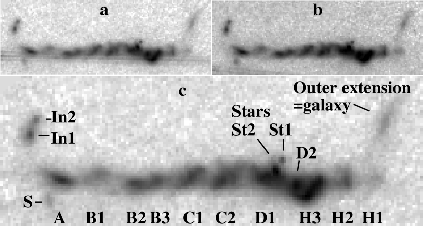
Figure 1: Map of near-infrared brightness ($\lambda 1.6\mu$m), rotated with position angle $222\degr$ along the horizontal. a: Sum of images with total exposure time 23 040 s, showing the diffraction spike passing through part of the jet. b: Sum of remaining images with total exposure time 11 520 s, diffraction spike clear of the jet. c: as a, after subtraction of diffraction spike modeled on b.

Figure 1 shows the reduced and summed images. The overall appearance of the jet’s morphology at 1.6 $\mu$m is very similar to that at visible wavelengths (compare the WFPC2 images in Jester et al. 2001, and Fig 2 below). The only significant difference (apart from the second star St2, see below) is that the tip of the jet H1 (apparently downstream of the hot spot H2) is visible on the infrared image, but not at higher frequencies. The jet appears equally well collimated in the near-infrared as in the optical. All optical extensions are detected, the southern extension S here being much weaker than knot A, while they are comparable in the UV. In1 is clearly brighter than In2, while again their near-UV brightness is comparable, indicating a marked color difference between the inner extension’s two knots.

There is signal from one of the quasar’s diffraction spikes superposed on the jet emission collected in the first 2/3 of the total exposure time (Fig. 1). In addition, an IR-bright object St2 is located within the jet, close to the faint star St1 just north of the jet which is also detected on the optical image. We modelled the spike by summing the 10 exposures in which the spike is clear of the jet (in these, the telescope has been rotated by 4° compared to the previous 20; Fig. 1 b). A scaled version of the model is then subtracted from each individual image. The result of subtracting the spike model from the “contaminated” sum frame is shown in Fig. 1 c.

To assess whether the IR-bright object St2 is part of the jet or an unrelated foreground object, we first checked whether its brightness profile is consistent with that of a point source. The widths of Gaussians fitted to 1D cuts along rows and columns of the sum images are consistent with the known width of the PSF. Secondly, there are no correlations with total or polarised brightness features of the radio jet. We are therefore confident that this object is a star which by chance appears superimposed on the jet image. We modelled this star on the sum images as a Gaussian sitting on top of a sloping plane which accounts for the underlying jet flux. An appropriately scaled version of the star model is subtracted from all 30 individual frames (for details, see Jester 2001, Section 2.2.5). The flux removed in this manner is $2.0\,\mbox{${\rm\thinspace\mu Jy}$}$. The jet flux in an equivalent aperture (ignoring any possible proper motion) on the F622W image of $0.2\,\mbox{${\rm\thinspace\mu Jy}$}$ is an upper limit to this object’s flux in this band, giving it a $R-H\ga 3$.

3 Photometry

In order to determine the synchrotron spectrum over the entire jet, we perform beam-matching aperture photometry at a grid of positions covering the jet. The photometry was done by our own MPIAPHOT software (cf. Röser & Meisenheimer 1991). This uses a weighted summation scheme, equivalent to a convolution, to match the different point spread functions to a common beam size. At the same time, it allows an arbitrary placement of apertures with respect to the pixel grid of individual images without loss of precision. All images are matched to a final resolution of 0$\aas@@fstack{\prime\prime}$3 FWHM, slightly inferior to that of the data set with the lowest resolution (the 3.6 cm radio data imaged with 0$\aas@@fstack{\prime\prime}$25 resolution; cf. §2.1). Following considerations given in Jester et al. (2001, Appendix A), this requires a relative image alignment accurate to 0$\aas@@fstack{\prime\prime}$03 in order to limit photometry errors from misalignment to 5% for point sources. The flanks of point sources have the steepest possible intensity gradients, the photometry error for extended sources will usually be an order of magnitude smaller. This accuracy is required to avoid the introduction of spurious spectral index features.

We achieve the desired alignment accuracy by using a grid of photometry positions, defined as offsets on the sky relative to the quasar core, which is assumed to coincide at all wavelengths. This grid is transformed into detector coordinates on each individual data frame, accounting for telescope offsets and geometric distortion. There is one frame each for the three VLA wavelengths, 30 for HST-NICMOS, four and 14, respectively, for HST-WFPC2 at 620${\rm\thinspace\,nm}$and 300${\rm\thinspace\,nm}$. Because of 3C 273’s location near the celestial equator, and because all offsets between individual HST frames are small (below 30″), detector and celestial coordinate offsets are related by a simple linear transformation.

The grid transformation is straightforward for the VLA images, which contain both the quasar and the jet and do not suffer from saturation effects. For the HST images, we first obtain the precise location of the quasar core from one short exposure (a few seconds) obtained during each HST “visit”. The telescope offsets between these short exposures and the deep science exposures of the jet are obtained from the engineering (“jitter”) files provided with the data. The aperture pixel position is calculated from the quasar’s pixel position, the desired offset on the sky and the telescope offset. We account for geometric distortion by using the wavelength-dependent cubic distortion correction for WFPC2 as determined by Trauger et al. (1995), and the quadratic NICMOS coefficients given in Cox et al. (1997). This procedure also takes care of the slightly differing image scales along the NIC2 detector’s x- and y-directions. We stress here that the unsaturated quasar image has been crucial in achieving the necessary alignment accuracy.

We use a rectangular grid of aperture positions. The grid extends along position angle 222$\aas@@fstack{\circ}$2, starting at a radial distance of $r=12\aas@@fstack{\prime\prime}0$ from the quasar and extending to $r=23\aas@@fstack{\prime\prime}0$. Perpendicular to the radius vector, the grid extends to $\pm 1\aas@@fstack{\prime\prime}0$. Individual grid points are spaced 0$\aas@@fstack{\prime\prime}$1 apart, yielding a good sampling of the 0$\aas@@fstack{\prime\prime}$3 effective resolution, so that there are 111 radial grid points and 21 points perpendicular to the radius vector, i. e., 2331 in total. All points are transferred to the individual data frames, and the flux per 0$\aas@@fstack{\prime\prime}$3 aperture centered at each grid position is determined.

The photon shot noise is below 0.5% per beam in all bands. The HST images have a flat-field error of 1% (WFPC2) and 3% (NICMOS) added in quadrature. The uncertainty in the background estimation is estimated from the scatter in blank sky regions as 0.01 $\mu$Jy per beam for WFPC2, and 0.03 $\mu$Jy for NICMOS, forming an error floor significant only for the faintest parts of the jet. An error source unique to the interferometric radio data is the error from the deconvolution, i.e., errors in the sense that the inferred brightness distribution does not correspond to the true distribution on sky, in particular for the fainter parts of the jet. This error is very hard to quantify and we use a 3% error to account for this. All these error sources limit the accuracy of relative photometry within one waveband. In addition, all wavebands will suffer an error from the absolute photometric calibration, typically 2%.

4 Results

4.1 Jet images at 0$\aas@@fstack{\prime\prime}$3

radius/″

$U$

300 nm

0.9${\rm\thinspace\mu Jy}$

$R$

620 nm

1.25${\rm\thinspace\mu Jy}$

$H$

1.6 $\mu$m

5.75${\rm\thinspace\mu Jy}$

K-band

1.3 cm

95${\rm\thinspace mJy}$

U-band

2.0 cm

150${\rm\thinspace mJy}$

X-band

3.6 cm

265${\rm\thinspace mJy}$

radius/″

Figure 2: Photometry of the jet in 3C 273 at 0$\aas@@fstack{\prime\prime}$3 effective beam size. Clipped to show only measurements with aperture signal-to-noise ratio $>5$. Grey levels runs from 0 to the peak flux/beam with a pseudo-logarithmic stretch as indicated by the greyscale bar. Jet features are labelled as in Fig. 1. The offset of 0$\aas@@fstack{\prime\prime}$2 between radio and optical hot spot position can be made out clearly.

In order to compare the images at different wavelengths, the photometry results are reassembled into the images shown in Fig. 2. We compare the jet’s morphological features at different wavelengths before considering the spectra.

4.1.1 Jet morphology from radio to UV

Figure 3: Plot of surface brightness per beam along the jet’s ridge line, i. e., showing the brightest point per column from Fig. 2.

Figure 4: Normalised cuts through the jet profile at various distances from the quasar at 300 nm (solid line), 620 nm (short dash), 1.6 $\mu$m (long dash), and 2.0 cm (dotted); resolution is 0$\aas@@fstack{\prime\prime}$3. Negative offsets are to the south of the jet. The shaded Gaussian in the first panel shows the resolution of 0$\aas@@fstack{\prime\prime}$3 FWHM. The “southern extension” is visible in the short-wavelength profiles at $r=12\aas@@fstack{\prime\prime}8$. However, the apparently corresponding feature in the radio profile is in fact unrelated. Instead, it is due to the radio cocoon around the jet: Röser et al. (1996, cf. their Fig. 3) noted that the radio emission is more extended, in particular to the south, than the optical emission. There is a similar tendency for the near-infrared profile to be more extended than the optical/UV. Other than that, the profiles show a similar jet width at all wavelengths. The cut through B1 clearly shows the transverse offset in optical and radio emission between the jet’s two strands. In D2, the radio peak appears offset slightly to the south from the optical peak, but the interpretation of this shift is uncertain.

To facilitate a comparison of the jet morphology at different wavelengths beyond a direct inspection of the panels in Fig. 2, we show the flux profile along the jet in Fig. 3 and normalised transverse profiles in 4. There is a close correspondence of morphological features at all wavelengths, i. e., a coincidence of local brightness maxima and the occurrence of “knots” across the entire observed wavelength range (cf. Bahcall et al. 1995, who describe the same fact by noting that the jet’s features have similar angular sizes at all wavelengths). The sole exception within the jet is region B1, in which the jet’s apparently double-stranded nature is most conspicuous. At HST frequencies, B1’s northern strand is considerably brighter than the southern, while on the radio images, the situation is exactly the opposite. This is also the only location in the jet which might be classified as edge-brightened (cf. §4.1.2). Note that the two bright knots of the jet preceding B1 are the sources of the brightest X-ray emission, perhaps with a small offset between the locations of the optical and X-ray peaks (Marshall et al. 2001).

Apart from this discrepancy, only the relative brightness of the knots changes with wavelength. Relative to knot A at the onset of the optical jet, the radio peak brightness increases by a factor of about 5–10 for H3, and another factor of two for the radio brightness peak H2, which has historically been called the radio “hot spot”. However, in the near-infrared at 1.6  $\mu$m, the brightness peaks at H3, and H2 are already fainter than most of the remainder of the jet. In the near-UV at 300${\rm\thinspace\,nm}$, H2 is the faintest feature, while A is the brightest. As already noted above, the tip of the jet H1 is detected up to the near-infrared, but not at shorter wavelengths (any emission so far detected at 600${\rm\thinspace\,nm}$beyond H2 is related to the nearby galaxy, not to H1). Thus, the brightness profile tends to invert from radio to near-ultraviolet. This trend continues up to X-rays: A dominates the jet’s X-ray luminosity (Marshall et al. 2001), while H2 dominates the radio luminosity. This change in brightness profile with wavelength is equivalent to a change in the spectrum along the jet, which will be considered below (§4.2).

The transverse cuts (Fig. 4) confirm the findings of Röser et al. (1996, cf. their Fig. 3): the width of the radio and optical jet is very similar, but there is extended radio emission without an optical counterpart to the south of the jet. Confirming the findings of Neumann et al. (1997a), there is a tendency for the near-infrared emission to be more extended to the south than the optical and ultraviolet emission. This strengthens their conclusion that the optical jet traces the emission of the jet channel as such. The more extended and fainter low-frequency emission corresponds to a surrounding cocoon of material, interpreted as material which is back-flowing after having passed through the hot spot (Röser et al. 1996).

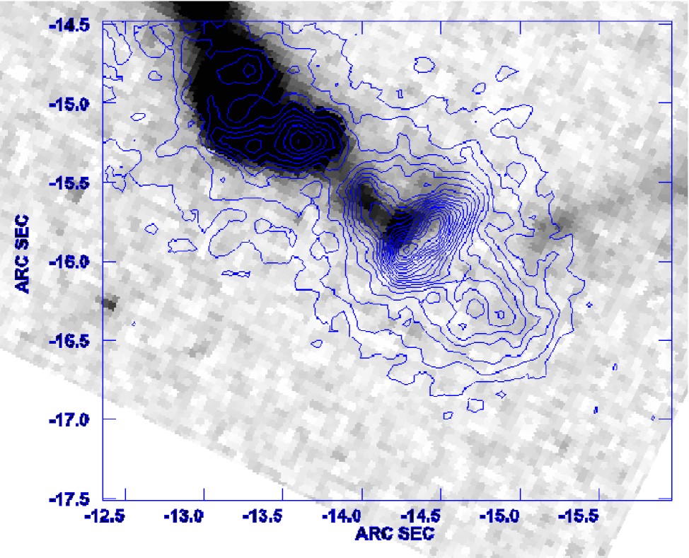
Figure 5: Comparison of hotspot position at optical and radio wavelengths. Greyscale shows the 620 nm image at original resolution, contours show the 1.3 cm radio map at 0$\aas@@fstack{\prime\prime}$125 resolution. Coordinates are relative to the quasar core, using which both images were aligned. The radio hot spot is clearly offset by 0$\aas@@fstack{\prime\prime}$2 from the optical hot spot, while the radio contours closely agree with the optical image in the preceding region (D2/H3).

Figures 2 and 3 show a radial offset of about 0$\aas@@fstack{\prime\prime}$2 between the position of H2 at radio and optical wavelengths. This offset is confirmed by the overlay of radio and optical data at the respective instrumental resolution in Fig. 5. The uncertainty of the offset determination is likely dominated by the systematic pointing uncertainty of the HST data with respect to the VLA data, which we kept to better than 0$\aas@@fstack{\prime\prime}$03 (cf. §3). We discuss the interpretation of this offset in §6.1.

4.1.2 Jet volume

It is necessary to know the jet volume to obtain an estimate for the magnetic field by the minimum-energy argument (§5.2 below). We just noted that the optical jet delineates the jet channel as such, while the radio emission contains contributions from the surrounding material. The geometry of the jet channel is therefore best constrained by considering the optical morphology. We assume the jet has isotropic emissivity which is constant along individual lines of sight through the jet and neglect relativistic beaming effects. (Even in the presence of beaming, the conclusions are unaltered as long as the beaming does not vary significantly along any given line of sight.)

The jet is center-brightened at all wavelengths on images resolving its width (the only exception being B1, as noted above in §4.1.1). If the emission region was confined to a cylindrical shell at the jet surface, the resulting brightness distribution would be edge-brightened, both for uniform emissivity resulting from a tangled magnetic field geometry, and for an ordered helical field (Meisenheimer 1990; Laing 1981). To lowest order, the jet is therefore considered as a cylinder completely filled with emitting plasma. The small-scale structure seen on the optical images and the 0$\aas@@fstack{\prime\prime}$2 optical spectral index map (Jester et al. 2001) suggests that the true internal structure of the jet is more complicated – so complicated that a more accurate model than the simple one assumed here requires a detailed understanding of the internal structure, composition and flow parameters governing the fluid dynamics of the jet. However, any model with more free parameters than a filled cylinder is not constrained by the available data. We therefore assume that the jet is a cylinder extending along position angle 222$\aas@@fstack{\circ}$2 whenever a value of the jet volume is required, and next determine the appropriate value for the radius of this cylinder.

4.1.3 Width of the jet

Figure 6: Comparison of jet full-width at half the maximum intensity at different wavelengths. The width is determined column by column on the images in Fig. 2 as the full width at half the maximum intensity along the column. The bottom panel shows the optical ($\lambda$620${\rm\thinspace\,nm}$) flux profile (maximum intensity) for reference. The middle panel shows the width at $\lambda$300 nm (UV), $\lambda 620$${\rm\thinspace\,nm}$(optical) and $\lambda 1.6\,\mu$m (IR). The upper panel shows again the optical width for reference and the width at the radio wavelengths of $\lambda 1.3\,$cm and $\lambda 2.0\,$cm. The right-hand-side axis for the upper two panels expresses the observed width in units of the effective resolution of 0$\aas@@fstack{\prime\prime}$3. This plot shows that although the jet is clearly wider in the radio than at HST frequencies, the increasing isophotal width in the radio is mainly caused by the increase in brightness, not by an actual widening, which would be seen as an increase in the jet’s FWHM.

Comparing the radio and the optical images (Fig. 2), it appears that the radio emission is widening significantly towards the hot spot, while the optical emission is of smaller and constant width. However, the transverse jet profiles (Fig. 4) show that the radio and optical width are, in fact, comparable throughout. The apparent widening of the radio isophotes is predominantly due to the increasing brightness, and hence and signal-to-noise ratio, as a larger part of the point spread function’s (PSF) wings is visible above the background noise. Finite-resolution isophotes should therefore not be used to judge the widths of jets.

With sufficient signal-to-noise, the appropriate comparison would be using a deconvolution. Here we instead give the run of the jet FWHM in Fig. 6. As expected from Fig. 4, the radio jet does not widen in the way suggested by its isophotal width, but the FWHM remains constant at roughly 1″(this was first noted by Conway et al. 1993).

One might hope to determine the true extent of the jet on the images or radio maps with the highest available resolution. While this is possible on the HST images for the entire jet, the resolution of $\approx 0\aas@@fstack{\prime\prime}1$ for the optical and $\approx 0\aas@@fstack{\prime\prime}2$ for the infrared is not reached by the VLA with sufficient signal-to-noise for most part of the jet. This is a consequence of the large dynamic range of over 30,000 between the fainter parts of the jet and the radio core. Therefore, the current radio data do not permit a comparison of the jet width at the resolution reached by HST. The dynamic range of these radio images actually fell short of expectations for reasons we are currently trying to understand.

Since the optical jet has fairly sharp boundaries on the WFPC2 $R$-band image at original resolution, we use the average width of the $3\sigma$ isophote of 0$\aas@@fstack{\prime\prime}$7 as the width of the jet channel (this is identical to the value reported by Bahcall et al. 1995). Thus, the jet channel is described as a cylinder of constant radius $0\aas@@fstack{\prime\prime}7/2=0\aas@@fstack{\prime\prime}35$ for regions A1–D2/H3 ($r=12\arcsec$–$21\arcsec$). This width agrees with the hot spot diameter given by Meisenheimer et al. (1997), so to lowest order, we can extend the cylindrical model to cover the entire jet out to the tip of the jet H1.

As the cocoon emission (cf. Fig. 4) is much fainter than the jet’s, its morphology is much more difficult to establish. To assess any likely contribution of the cocoon emission to the flux observed from the jet, the radio emission surrounding the optical jet channel is described as a cylindrical shell with inner radius 0$\aas@@fstack{\prime\prime}$35 (enclosing the optical jet channel without a gap) and outer radius 0$\aas@@fstack{\prime\prime}$8, close to the isophotal width of the radio jet there and roughly twice that of the optical jet.

The volume belonging to each photometry aperture (or pixel in Fig. 2), i. e., the effective jet volume sampled by each photometry aperture, is calculated by explicitly convolving the model assumed for the jet (a filled cylinder of radius 0$\aas@@fstack{\prime\prime}$35) with the observing beam of 0$\aas@@fstack{\prime\prime}$3 FWHM at the location of each aperture, assuming that the symmetry axis of the cylinder lies along the radius vector at position angle 222$\aas@@fstack{\circ}$2. The obtained values are tabulated in Tab. 2. We use them here to assess the likely relative volume emissivity of the jet and the cocoon. The jet volume sampled by each aperture will be used in the calculation of the minimum-energy field in §5.2, where we also consider the effect of the inclination of the jet to the line of sight.

Table 2: Effective volume of the jet sampled by photometry apertures at distance $\delta_{\mathrm{y}}$ from the symmetry axis of the model. Jet volume, contribution from the jet channel visible in the optical, assumed as filled cylinder extending from $\delta_{\mathrm{y}}=0\arcsec$ to $\delta_{\mathrm{y}}=0\aas@@fstack{\prime\prime}35$. Cocoon volume, contribution from the cocoon, modelled as hollow cylinder wrapped extending from $\delta_{\mathrm{y}}=0\aas@@fstack{\prime\prime}35$ to $\delta_{\mathrm{y}}=1\arcsec$ around the jet channel. These values assume a fully side-on view.

$\delta_{\mathrm{y}}$	Jet volume	Cocoon volume
″	$(h_{70}^{-1}\mbox{${\rm\thinspace kpc}$})^{3}$	$(h_{70}^{-1}\mbox{${\rm\thinspace kpc}$})^{3}$
0.0	1.3	1.8
0.1	1.2	1.9
0.2	.98	2.0
0.3	.62	2.3
0.4	.28	2.4
0.5	.084	2.3
0.6	.015	1.9
0.7	.0016	1.3
0.8	.0001	.71
0.9	.00003	.26
1.0	.0000007	.06

Using Tab. 2, we can now also estimate the contribution of the cocoon or backflow material along the line of sight to the central part of the jet. The effective volume contributed by the cocoon volume is much larger than that of the jet channel. Therefore, the cocoon’s volume emissivity can be no more than about 1% of the jet’s volume emissivity (the exact ratio depends on the azimuthal extent of the cocoon). Otherwise, the cocoon emission would completely dominate the jet emission and the profile would not appear centrally peaked, or fall off more slowly than observed. In the central part of the jet, the cocoon will then also contribute only about 1% of the jet emission. The same constraint from the observed brightness profile implies that the contribution of the cocoon to the central jet flux cannot be appreciable even if the true width of the cocoon is different from the assumed 0$\aas@@fstack{\prime\prime}$8.

4.1.4 Morphology summary

In summary, the overall morphology of the jet is similar at all observed wavelengths from 3.6 cm to 300 nm. The exceptions to this are the radio-quiet “extensions” (In1, In2, S; Fig.1 and Jester et al. 2001) to the optical jet, and region B1, in which the SED of the southern strand of emission peaks in the radio, but that of the northern strand peaks at optical wavelengths. All of the emission blueward of 1.6 $\mu$m and the bulk of the radio emission at the wavelengths of 3.6${\rm\thinspace cm}$ and shorter considered here are emission from the jet itself, while the steep-spectrum radio cocoon (or “backflow”) south of the jet makes a negligible contribution along the line of sight to the jet channel (cf.  Conway et al. 1993; Conway & Davis 1994). We therefore use the full data set from 3.6${\rm\thinspace cm}$ to 300${\rm\thinspace\,nm}$ to analyse the spectrum of the jet emission here.

4.2 Spectral indices

a)

$-2$…0

$\alpha^{\mathrm{UV}}_{\mathrm{opt}}$

$\frac{300\,\mathrm{nm}}{620\,\mathrm{nm}}$

b)

$-2.5$…

…$-0.4$

$\alpha^{\mathrm{opt}}_{\mathrm{IR}}$

$\frac{620\,\mathrm{nm}}{1.6\,\mu\mathrm{m}}$

c)

$-1.35$…

…$-0.8$

$\alpha^{\mathrm{IR}}_{\mathrm{1.3}}$

$\frac{1.6\,\mu\mathrm{m}}{1.3\,\mathrm{cm}}$

d)

$-2$…0

$\alpha^{\mathrm{1.3}}_{\mathrm{2.0}}$

$\frac{1.3\,\mathrm{cm}}{2.0\,\mathrm{cm}}$

e)

$-2$…0

$\alpha^{\mathrm{2.0}}_{\mathrm{3.6}}$

$\frac{2.0\,\mathrm{cm}}{3.6\,\mathrm{cm}}$

radius/″

Figure 7: Spectral index maps at 0$\aas@@fstack{\prime\prime}$3 resolution generated from the photometry data in Fig. 2. Only pixels with a signal-to-noise ratio of at least 5 per beam are shown. Images are combined pairwise in order of increasing wavelength. Linear colour scales (shown above the respective images) have been chosen to stress variations within one map.
a, optical spectral index (range: $-2$…$0$); b, optical-infrared ($-2.5$…$-0.4$); c, infrared-radio ($-1.35$…$-0.8$); d, radio $\lambda 1.3\,$cm-$\lambda 2.0\,$cm ($-2$…$0$); e, radio $\lambda 2.0\,$cm-$\lambda 3.6\,$cm ($-2$…$0$)
The variations of both radio spectral indices in the inner part of the jet are mainly due to low signal-to-noise and the associated imaging uncertainties. Compare with Fig. 8 to gauge the relative magnitude of variations of the different spectral indices.

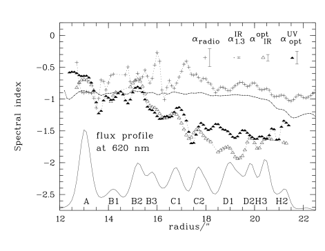
Figure 8: Run of the spectral indices along the jet at 0$\aas@@fstack{\prime\prime}$3 resolution, sampled in 0$\aas@@fstack{\prime\prime}$1 intervals (cut along radius vector at position angle 222$\aas@@fstack{\circ}$2). For sake of clarity, only typical $2\sigma$ error bars are shown for the random error. Systematic flux calibration uncertainties are of the same order and would shift an entire curve. The radio spectral index $\alpha_{\mathrm{radio}}$ is obtained by a fit to the radio data at 3.6${\rm\thinspace cm}$, 2.0${\rm\thinspace cm}$, and 1.3${\rm\thinspace cm}$. The other spectral indices are derived from the jet photometry at the given wavelengths ($\alpha_{1.3}^{\mathrm{IR}}$: 1.3${\rm\thinspace cm}$ and 1.6 $\mu$m, $\alpha^{\mathrm{opt}}_{\mathrm{IR}}$: 1.6 $\mu$m and 620${\rm\thinspace\,nm}$, $\alpha^{\mathrm{UV}}_{\mathrm{opt}}$: 620${\rm\thinspace\,nm}$ and 300${\rm\thinspace\,nm}$). The optical flux profile is shown for reference. Reprinted from Jester et al. (2002) for reference.

From the photometry results shown in Fig. 2, we compute pairwise spectral indices $\alpha$. The spectral index maps are shown in Fig. 7. Their run along the jet’s centre line is shown in Fig. 8 (Fig. 1 in Jester et al. 2002). The error bars in Fig. 8 have been calculated from the total random error. There is an additional systematic error from flux calibration uncertainties (typically 2%, §3). These change all flux measurements through one filter by the same factor. Its effect on the spectral index determination is to offset a given spectral index by a constant amount for the entire jet. The magnitude of the effect is smaller than any of features which we detect at high statistical significance. Our conclusions are, therefore, unaffected by this residual systematic uncertainty.

The two radio spectral indices (between 3.6${\rm\thinspace cm}$ and 2${\rm\thinspace cm}$, and between 2${\rm\thinspace cm}$ and 1.3${\rm\thinspace cm}$) behave erratically out to a radius of about 19″. These variations are not significant: the radio jet is detected at low signal-to-noise ratio at the inner end, and the deconvolution involved in the reconstruction of the brightness distribution on the sky from the observed interferometric data is only accurate (in the sense of achieving an image representing the true brightness distribution) for high signal-to-noise. We therefore show an overall radio spectral index in Fig. 8 which has been determined by a least-squares straight-line fit to the three radio data points. For the outer part of the jet, the radio spectral index shows a steepening of the hot spot (H2) spectrum compared to the remainder of the jet. The run of the spectral index between 6${\rm\thinspace cm}$ and 3.6${\rm\thinspace cm}$, for which only lower-resolution data at 0$\aas@@fstack{\prime\prime}$5 are available agrees with the spectral index run determined at the wavelengths considered here (cf. Conway et al. 1993).

The infrared-radio spectral index (Fig. 7c) is nearly constant at $\mbox{$\alpha^{\mathrm{IR}}_{\mathrm{radio}}$}\approx-0.9$ along the centre of the optical jet, with some flattening in optically bright regions and a pronounced steepening in the transition from D2 ($r\approx 20\arcsec$) to the radio hot spot H2. It steepens markedly to $\approx-1.2$ away from the centre line. These features are identical to those identified by Neumann et al. (1997a) on a spectral index map at 1$\aas@@fstack{\prime\prime}$3 resolution generated from observations at 73${\rm\thinspace cm}$ and 2.1 $\mu$m. There is no spectral index feature uniquely corresponding to the hot spot H2, as is the case on the radio spectral index map. On the other hand, the tip of the jet H1 is identifiable as region with radio-infrared spectral index slightly flatter than H2.

We use the term “high-frequency” to refer to the infrared-optical and optical-ultraviolet spectral indices. As already noted by considering the spectral index map derived from the optical and near-ultraviolet imaging at 0$\aas@@fstack{\prime\prime}$2 resolution (Jester et al. 2001), there are none but smooth changes in the optical-UV spectral index along the jet. The same is true for the infrared-optical spectral index. Both these spectral indices decline globally along the jet. At the onset of the optical jet at A and at B1, both have a value of $-0.7$, i. e., the optical-UV spectrum there is flatter than the radio and radio-infrared. Both high-frequency indices decrease to about $-1.7$ at C2. The optical-ultraviolet $\alpha^{\mathrm{UV}}_{\mathrm{opt}}$ remains near this value for the reminder of the jet, while the infrared-optical $\alpha^{\mathrm{opt}}_{\mathrm{IR}}$ steepens further, reaching a minimum near $-2$ between D1 and D2, and flattening back to $-1.7$ at D2.

Thus, as already reported in Jester et al. (2002), the spectrum does not steepen everywhere towards higher frequencies, but flattens between the near-infrared and optical in nearly all parts of the jet. We will consider the implications of this finding in §§5 and 6.2.

Figure 9: Comparison of high-frequency spectral indices with previous observations at 1$\aas@@fstack{\prime\prime}$3 resolution. Top, comparison of optical spectral index $\alpha_{BRI}$ at 1$\aas@@fstack{\prime\prime}$3 resolution from Röser & Meisenheimer (1991) with optical-UV spectral index $\alpha^{\mathrm{UV}}_{\mathrm{opt}}$ at 0$\aas@@fstack{\prime\prime}$3 from this work (error bars are similar for $\alpha_{BRI}$ and $\alpha^{\mathrm{UV}}_{\mathrm{opt}}$). Below, comparison of infrared-optical spectral index $\alpha_{\mathrm{KO}}$ from Neumann et al. (1997a) and $\alpha^{\mathrm{opt}}_{\mathrm{IR}}$ from this work (only every tenth error bar shown). The overall agreement between the spectral indices at 0$\aas@@fstack{\prime\prime}$3 and 1$\aas@@fstack{\prime\prime}$3 is surprisingly good. Differences between $\alpha^{\mathrm{UV}}_{\mathrm{opt}}$ and $\alpha_{BRI}$ occur in A, C2, D1, and D2, those regions in which the observed spectrum (Fig.8) does not show the expected steepening towards higher frequencies.

The general outward steepening of the high-frequency spectral indices is in agreement with previous determinations of the knots’ synchrotron spectrum which showed a decrease of the cutoff frequency outward (Meisenheimer et al. 1996a; Röser et al. 2000). There is an excellent correspondence of the run of the optical-infrared spectral index $\alpha^{\mathrm{opt}}_{\mathrm{IR}}$ along the jet with the spectral index $\alpha_{\mathrm{KO}}$ between $2.1\,\mu$m and the optical as determined by Neumann et al. (1997a) at 1$\aas@@fstack{\prime\prime}$3 resolution (Fig. 9). As has been noted in Jester et al. (2001), the overall run of the optical-ultraviolet spectral index $\alpha^{\mathrm{UV}}_{\mathrm{opt}}$ at 0$\aas@@fstack{\prime\prime}$3 agrees overall with the run of the optical spectral index $\alpha_{BRI}$ at 1$\aas@@fstack{\prime\prime}$3, with discrepancies in a few regiosn: a comparison of Figs. 8 and 9 shows that these discrepancies arise precisely in those regions in which the spectrum flattens at high frequencies. The discrepancies can thus be ascribed to the different wavelength of the bluest HST and ground-based images (300 nm compared to 400 nm) and the fact that the flattening occurs just in this wavelength region (between 600 to 300 nm).

Optical spectral index variations are not strongly correlated with brightness variations. Some local peaks of $\alpha^{\mathrm{UV}}_{\mathrm{opt}}$ coincide with brightness maxima, while others coincide with minima. In contrast, there is a correlation between the optical-infrared spectral index $\alpha^{\mathrm{opt}}_{\mathrm{IR}}$ and the jet’s surface brightness, in the sense that brighter regions show a flatter spectrum (smaller $|\mbox{$\alpha^{\mathrm{opt}}_{\mathrm{IR}}$}|$, see Figs. 7 b and 8). This correlation is most clearly visible on the spectral index map for the outer end of the jet. The bright regions D2/H3 together with the hot spot H2 appear as an island of $\mbox{$\alpha^{\mathrm{opt}}_{\mathrm{IR}}$}\approx-1.6$ surrounded by regions with steeper spectrum. The correlation between local maxima in surface brightness and $\alpha^{\mathrm{opt}}_{\mathrm{IR}}$ is also present in the inner part of the jet, although the spectral index maxima are displaced sideways from the brightness peaks due to a transverse spectral index gradient.

This spectral index gradient is suggestive of a residual misalignment between the optical and infrared images, e. g., a rotation between the two about a point close to D2/H3. It could also have been caused by an overestimation of the diffraction spike signal which has been modelled and subtracted (see §2.3.2). Since Neumann et al. (1997a) did not detect a significant change of the infrared-optical spectral index transversely to the jet at 1$\aas@@fstack{\prime\prime}$3, and although the alignment procedures described above (§3) should have ensured that such an error should not have occurred, we reconsidered this possibility to avoid the introduction of spurious gradients. After a detailed investigation (details are contained in Jester 2001), we concluded that the misalignment necessary to produce such a gradient was far greater than compatible with the alignment precision established previously. Neither can the gradient firmly be linked to the diffraction spike subtraction or any obviously detectable misalignment. In the given situation, we rely on the data with the offsets established to the best of our knowledge. The clarification of this matter has to await new observational data.

In summary, there are two surprising findings regarding the spectral indices. Firstly, the knots, i. e., the local brightness peaks occurring at nearly the same position at all wavelengths, have a flatter infrared-optical spectrum than the regions separating them. Thus, there is a local positive correlation between the jet brightness at any wavelength and the infrared-optical spectral index. This contrasts with the global anti-correlation between energy output and spectral index: the radio surface brightness increases while the high-frequency spectrum steepens considerably. Secondly, the spectrum flattens in the optical-UV wavelength region. In fact, the optical-ultraviolet $\alpha^{\mathrm{UV}}_{\mathrm{opt}}$ spectral index is nowhere significantly below the infrared-optical $\alpha^{\mathrm{opt}}_{\mathrm{IR}}$, in contrast to the expectation of a synchrotron spectrum which steepens at higher frequencies. We will consider the implications in §6.4 and first turn to the determination of the maximum particle energy from the observations.

5 Analysis

The present observations have been obtained to study the behaviour of the maximum particle energy along the jet in 3C 273, with the aim of identifying acceleration and/or loss sites within the jet. In order to determine the maximum particle energy from the observed spectral energy distributions, we need to determine both the cutoff frequency $\nu_{\mathrm{c}}$  which is the characteristic synchrotron frequency corresponding to the highest particle energy, and the magnetic field in the jet, assumed to be uniform along lines of sight. We first consider the determination of the cutoff frequency and then estimate the magnetic field strength using the minimum-energy argument in §5.2.

5.1 Spectral fits: determination of $\nu_{\mathrm{c}}$

The cutoff frequency is to be determined from the observed spectral energy distributions by fitting them with model synchrotron spectra. All previous studies have used single-population models to describe the jet’s synchrotron spectrum (Röser et al. 2000; Meisenheimer et al. 1996a; Neumann et al. 1997a; Meisenheimer et al. 1997). We noted above that there is a flattening of the observed spectrum towards the ultraviolet (Fig. 8 in §4.2). This means that a description using a single electron population is, in fact, inadequate: any non-idealised power-law electron population (i.e., with finite maximum particle energy and rapid pitch-angle scattering) always gives rise to a synchrotron spectrum with steepening slope in the $\log B_{\nu}$–$\log\nu$ plane. The observed high-frequency flattening implies that a second high-frequency emission component must be present, which contributes either predominantly to the jet’s near-infrared or near-ultraviolet flux to produce the observed high-frequency flattening. The discrepancy can be explained by assuming that one of the two spectral indices reflects the true synchrotron spectrum, while the other is contaminated by flux not due to the same population as the remainder of the jet. To assess the likely reason for this discrepancy between the observations and the expectations from synchrotron theory, we perform two separate fits which differ in the determination of the cutoff frequency (Fig. 10): either the cutoff is described by the optical-ultraviolet spectral index leading to an infrared excess (Model A), or conversely, the true cutoff is described by the infrared-optical spectrum and there is additional flux in the ultraviolet (Model B; see Jester et al. 2002). This allows us to perform the fits using a single-population model.

Following previous studies, we use the method of computing synchrotron spectra with a smooth cutoff from Heavens & Meisenheimer (1987) to determine the cutoff frequency from the observed spectral energy distribution. They model the synchrotron source as a region of constant magnetic field into which a power-law distribution of electrons extending up to a maximum electron Lorentz factor $\gamma_{\mathrm{max}}$ is continuously injected. The resulting spectrum has a low-frequency power law part with spectral index $\alpha_{\mathrm{low}}$, which steepens by one-half power at a break frequency $\nu_{\mathrm{b}}$ and cuts off exponentially above the cutoff frequency $\mbox{$\nu_{\mathrm{c}}$}>\mbox{$\nu_{\mathrm{b}}$}$. The break is produced by adding up the contributions from the electron population observed at increasing times since acceleration, i. e., with different cutoff frequencies. The magnitude of the break of $1/2$ is fixed by the cooling mechanism. Although the model was originally devised to describe the spectra of hot spots, the use of such a continuous-injection model is justified by the fact that optically emitting electrons must be accelerated within the jet: our calculation in Jester et al. (2001) showed that relativistic beaming and/or sub-equipartition magnetic fields cannot remove the discrepancy between light-travel time along 3C 273’s jet and the lifetime of electrons emitting optical synchrotron radiation.

The model spectrum has four free parameters: the low-frequency spectral index $\alpha_{\mathrm{low}}$, the ratio of cutoff energy to break energy of the emitting electron population = $\sqrt{\mbox{$\nu_{\mathrm{c}}$}/\mbox{$\nu_{\mathrm{b}}$}}$, the observed cutoff frequency $\nu_{\mathrm{c}}$, and a flux normalisation. Since we only observe the spectrum at six frequencies, we introduce additional constraints to obtain meaningful fits. First, we restrict $\sqrt{\mbox{$\nu_{\mathrm{c}}$}/\mbox{$\nu_{\mathrm{b}}$}}$ so that the break is in the range $10^{9}$ Hz–$10^{12}$ Hz, i. e., within the range of the observed radio data. Secondly, we artificially fix $\alpha_{\mathrm{low}}\approx-0.4$, so that the observed radio-infrared spectral index of about $-0.9$ (Fig. 8) corresponds to $\alpha_{\mathrm{low}}-0.5$. In effect, only the cutoff frequency $\nu_{\mathrm{c}}$ is determined by this fitting procedure. The fit is performed using a $\chi^{2}$ minimisation technique; the detailed steps can be found in Jester (2001, §4.2 and references therein). We discuss the implications of these constraints on the interpretation of the fit results in §5.3 below.

5.1.1 Model A and Model B

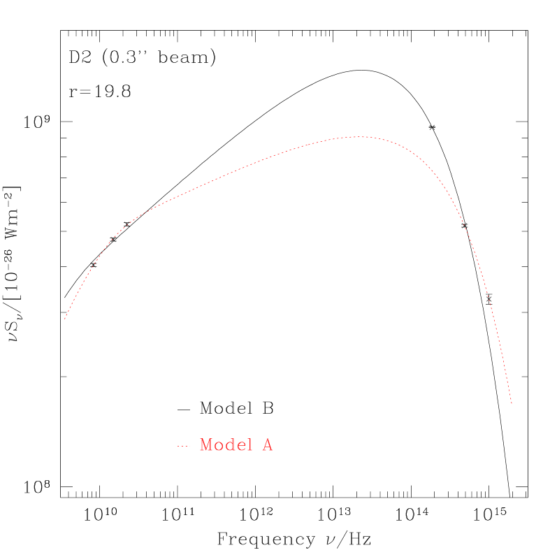
Figure 10: Illustration of the two different spectral fits performed. Model A assumes infrared emission in excess of the cutoff given by the optical-ultraviolet spectral index, while Model B assumes an ultraviolet excess above the infrared-optical cutoff.

Model A assigns a low weight to the near-infrared flux point in the data set. This is motivated by the indication that the radio cocoon (possibly a “backflow”) around the jet (Röser et al. 1996) may also be detectable at 2.1 $\mu$m (Neumann et al. 1997a), suggesting that the flux from the jet at 1.6 $\mu$m may be contaminated by emission from the cocoon as well. Hence, the cutoff in Model A is determined by the optical and near-ultraviolet points at 620${\rm\thinspace\,nm}$ and 300${\rm\thinspace\,nm}$, respectively. Conversely, in Model B, the location of the cutoff is dominated by the infrared and optical points at 1.6 $\mu$m and 620${\rm\thinspace\,nm}$, respectively.

In contrast to the remainder of the jet, the hot spot shows an offset between optical and radio hot spot position (Fig. 5) and a change of the radio-infrared spectral index (§4.2). Therefore, the spectra from the hot spot regions H2 and H1 at radii beyond $r=21\arcsec$ are fitted differently by allowing $\alpha_{\mathrm{low}}$ to vary between $-0.8$ and $-0.3$. This model is referred to as Model HS.

In the bright peaks of A, B1 and B2, there is no cutoff within the observed frequency range (the high-frequency spectral indices are flatter than $-1$ there (Fig. 8), so that the spectral energy density continues to rise towards higher frequencies). Where this is the case, an artificial high-frequency data point is introduced to allow the fit to proceed, which assumes the presence of a local maximum in the data set. The artificial point is chosen so that it has a spectral index relative to the observed UV point of $-1.2$ and is introduced at a frequency $10^{18}$ Hz, 1000 times higher than the frequency of UV emission. It is assigned a large error so that it does not influence the goodness-of-fit. The results obtained for $\nu_{\mathrm{c}}$ for these points are then only lower limits to the true cutoff frequency as it would be inferred from observations at higher frequencies. On the other hand, it is possible that the optical/UV emission in these regions has a substantial contribution from the second, high-energy emission component (§6.2). In this case, there may be a cutoff to the “low-energy” radio-optical synchrotron component at lower energies than obtained here. Observations in additional wavebands, in particular at longer infrared wavelengths, or a comparison of the radio and optical polarisation of these regions at high resolution may shed light on this issue. However, given the similarity of radio and optical polarisation at low resolution, it appears unlikely that the emission is dominated by the high-energy component, although its contribution may be significant.

5.1.2 Fit results

Figure 11: Location of apertures for which spectra are shown in Fig. 12. Locations at local peaks (“knots”) are marked by a line below the image, while locations in inter-knot regions are marked by a line above.

At the chosen resolution of 0$\aas@@fstack{\prime\prime}$3, the inter-knot regions are fairly well-resolved from the knots themselves, so that we obtain meaningful values for the cutoff frequency for the entire jet. For the following discussion, we have chosen 16 locations corresponding to distinct features, the inter-knot regions and the brightness peaks. These locations are indicated in Fig. 11. Figure 12 shows the corresponding spectra, table 3 shows the fit parameters describing the shape of the spectrum (low-frequency spectral index, break frequency, cutoff frequency).

The fit results for the Models A and B are very similar in most cases. As described in detail in Jester et al. (2002, section 3), we reject the large near-infrared residuals obtained with Model A as implausible and prefer Model B, which has a significant excess in the near-UV. This implies that the jet emission consists of a “low-frequency” component responsible for emission from radio through optical, and at least one “high-energy” component, responsible for the near-UV emission, and possibly the X-rays at well. We will nevertheless show all results for both models to illustrate that the quantities derived from either model do not differ significantly.

Table 3: Fit parameters describing the shape of the spectra (low-frequency spectral index, break frequency, cutoff frequency) shown in Fig. 12.

			Model A			Model B/HS
Location	$r$	$\delta_{\mathrm{y}}$	$\alpha_{\mathrm{low}}$	$\nu_{\mathrm{b}}$	$\nu_{\mathrm{c}}$	$\alpha_{\mathrm{low}}$	$\nu_{\mathrm{b}}$	$\nu_{\mathrm{c}}$
	″	″		Hz	Hz		Hz	Hz
A	13.0	0.0	$-$0.35	$1.83\times 10^{10}$	$1.83\times 10^{16}$ $\dagger$	…	…	…
A-B1	13.7	0.0	$-$0.38	$2.25\times 10^{9}$	$2.25\times 10^{15}$	$-$0.38	$2.15\times 10^{9}$	$2.15\times 10^{15}$
B1	14.2	0.1	$-$0.35	$7.13\times 10^{9}$	$7.14\times 10^{15}$ $\dagger$	…	…	…
B2	15.2	$-$0.1	$-$0.44	$2.78\times 10^{11}$	$3.81\times 10^{16}$ $\dagger$	…	…	…
B3	15.6	$-$0.1	$-$0.48	$2.71\times 10^{11}$	$3.34\times 10^{16}$	$-$0.46	$1.98\times 10^{11}$	$2.38\times 10^{16}$
B3-C1	16.3	0.0	$-$0.38	$3.12\times 10^{9}$	$3.13\times 10^{15}$	$-$0.35	$1.36\times 10^{9}$	$1.36\times 10^{15}$
C1	16.8	0.1	$-$0.39	$1.65\times 10^{10}$	$5.24\times 10^{15}$	$-$0.38	$1.59\times 10^{10}$	$3.74\times 10^{15}$
C1-C2	17.3	0.0	$-$0.37	$1.45\times 10^{11}$	$4.42\times 10^{14}$	$-$0.35	$1.35\times 10^{11}$	$3.67\times 10^{14}$
C2	17.7	0.0	$-$0.36	$2.86\times 10^{10}$	$9.38\times 10^{14}$	$-$0.35	$3.07\times 10^{10}$	$8.19\times 10^{14}$
C2-D1	18.3	0.2	$-$0.49	$2.39\times 10^{10}$	$7.88\times 10^{15}$	$-$0.35	$8.65\times 10^{9}$	$5.46\times 10^{14}$
D1	18.9	0.1	$-$0.48	$1.06\times 10^{10}$	$4.34\times 10^{15}$	$-$0.35	$9.58\times 10^{8}$	$4.65\times 10^{14}$
D1-D2	19.5	$-$0.2	$-$0.35	$4.62\times 10^{9}$	$3.16\times 10^{14}$	$-$0.35	$5.78\times 10^{9}$	$3.23\times 10^{14}$
D2	19.8	$-$0.2	$-$0.35	$7.92\times 10^{9}$	$5.26\times 10^{14}$	$-$0.35	$9.27\times 10^{9}$	$5.15\times 10^{14}$
H3	20.2	$-$0.3	$-$0.39	$2.20\times 10^{9}$	$8.75\times 10^{14}$	$-$0.35	$1.08\times 10^{9}$	$5.10\times 10^{14}$
H2	21.3	0.0	…	…	…	$-$0.60	$1.14\times 10^{10}$	$7.50\times 10^{14}$
H1	22.1	$-$0.2	…	…	…	$-$0.44	$2.28\times 10^{9}$	$5.79\times 10^{13}$

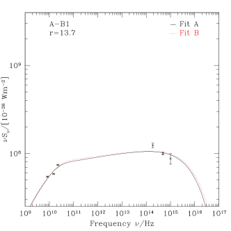
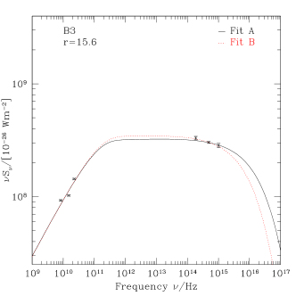
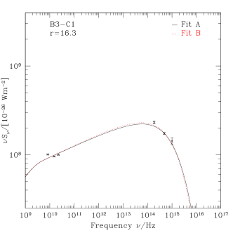
Figure 12: Observed data points with fitted spectra for the points shown in Fig. 11. To account for the observed flattening of the spectrum towards the ultraviolet, Model A assumes a contamination in the infrared, so that the cutoff is determined by the optical-ultraviolet spectral index there, while the cutoff in Model B is determined by the infrared-optical spectral index. Those spectra which require an artificial high-frequency data point to obtain a fit result are labelled “cut”; for these, Model A and Model B are identical, and the artificially obtained value for $\nu_{\mathrm{c}}$ is a lower limit to the actual value. The spectrum may extend up to X-rays in those locations where an artificial cut is necessary (cf. Röser et al. 2000; Marshall et al. 2001; Jester et al. 2002). Continues.

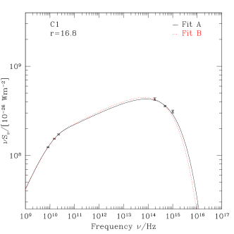
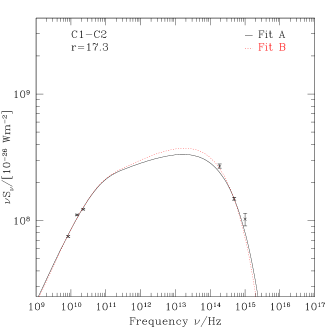
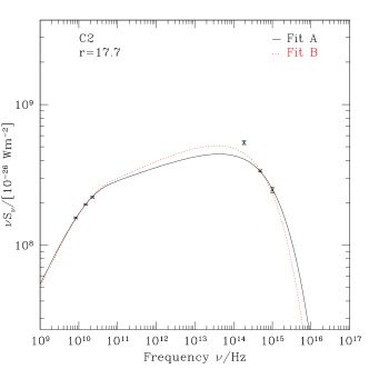
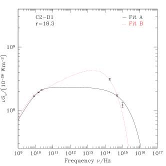
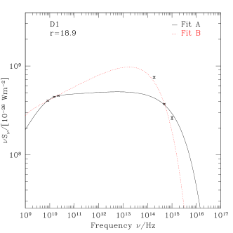
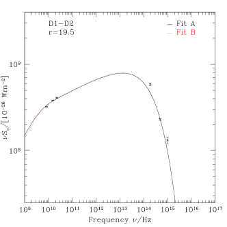
Figure 13: As Fig. 12, continued

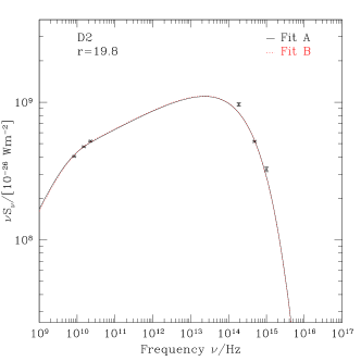
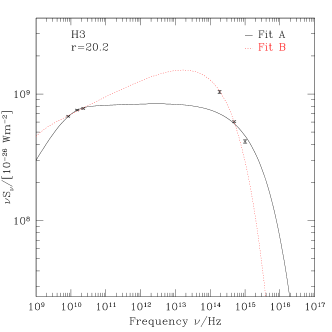
Figure 14: As Fig. 12, continued

Figure 12 highlights the development of the spectra along the jet: a global increase in luminosity coupled with a decrease in cutoff frequency. As expected from the brightness profiles, the spectral energy distribution peaks at lower frequencies at larger radii from the core. Simultaneously, the peak flux density increases.

Compared to earlier studies at lower resolution (Meisenheimer et al. 1996a; Neumann 1995; Röser et al. 2000), the contributions from individual knots are now clearly separated from each other. While previously only knot A showed a spectrum without a cutoff, it is now seen that there is no cutoff at the brightness peaks in B1 and B2, either. Not only is there no cutoff, but the infrared-optical-UV spectrum is harder than the radio-infrared spectrum in these locations, as already inferred from the spectral indices (compare Fig. 8). There is, however, a cutoff in the transition A-B1, between these peaks. The presence of a cutoff in the southern part of B1 can already be inferred from the fact that it is optically much fainter than the northern part, while it is brighter in the radio (cf. Fig. 2). The differences between the spectra fitted at the brightness peaks and the regions connecting them are nowhere else as drastic. However, for the first time we see that there is an increase of the cutoff frequency in the knots, compared to inter-knot regions, corresponding to the slightly flatter spectrum there (cf. §4.2). This local increase is a modulation of the global outward decrease of the cutoff frequency.

The synchrotron radiation at the cutoff frequency is emitted by those particles with the highest energy. The maximum particle energy can therefore be computed from the cutoff frequency through the synchrotron characteristic frequency, the frequency around which most of the synchrotron emission of an electron of energy $\gamma m_{\mathrm{e}}c^{2}$ in a magnetic field of flux density $B$ is emitted:

$$\nu_{\mathrm{char}}=4.2\times 10^{15}\left(\frac{\gamma}{10^{7}}\right)^{2}\left(\frac{B\sin\psi}{\rm nT}\right){\rm Hz}.$$ (1)

The dependence on the pitch angle $\psi$ requires one to make an assumption about the pitch angle distribution, which we take to be isotropic. This calculation requires the knowledge of the magnetic field in the source. In order to discuss the behaviour of the cutoff frequency and the maximum particle energy together, we first consider how to derive the magnetic field value.

In the absence of any other reliable method, the magnetic field for the jet can only be estimated by making use of the minimum-energy assumption. We therefore present the derivation of the value of the minimum-energy magnetic field for the type of spectra described here.

5.2 Equipartition field strength

There is a firm minimum value for the total energy density (in relativistic particles and magnetic field) necessary to generate a given synchrotron luminosity. This energy density can be deduced from observations with the help of assumptions about the source geometry and the range of frequencies over which synchrotron emission is emitted. Pacholczyk (1970) presents a clear derivation of the minimum energy density of a synchrotron source for the assumption of a power-law electron energy distribution in the source.

The minimum-energy field is that value of the source’s magnetic field corresponding to the minimum total energy sufficient to give the observed emission. Due to the lack of other diagnostic tools, this minimum-energy magnetic field is often used as estimate for the true magnetic field. Doing so, one introduces a local correlation between the magnetic field strength and the energy density in particles. This correlation provides the most efficient way to produce a given synchrotron luminosity. One may imagine magneto-hydrodynamical processes causing this correlation, because the particles are both tied to magnetic field lines and create them by their motion. However, no detailed microphysical feedback process has been identified which maintains this correlation on all scales, and it appears dangerous to us to draw conclusions deriving from this correlation until it is is established that it is a natural, not an artificial one. Nevertheless, it seems reasonable to assume that the minimum-energy magnetic field is a good indicator of the order of magnitude of the source’s magnetic field (Meisenheimer et al. 1989).

With this caveat in mind, we use the minimum-energy magnetic field as a measure of the jet’s magnetic field, calculating it following Pacholczyk (1970, p. 168 ff.) but explicitly assuming a broken power law. To account for the break in the electron spectrum at Lorentz factor $\gamma_{\mathrm{b}}$ leading to a break in the model spectrum at $\nu_{\mathrm{b}}$, we write the electron density as

$$n(\gamma)=\left\{\begin{array}[]{l@{\mathrm{\ for\ }}r}n(\gamma_{0})\left(\frac{\gamma}{\gamma_{0}}\right)^{-p_{\mathrm{low}}}&\gamma<\gamma_{\mathrm{b}}\\ n(\gamma_{0})\left(\frac{\gamma}{\gamma_{0}}\right)^{-p_{\mathrm{high}}}&\gamma\geq\gamma_{\mathrm{b}}\end{array}\right.$$ (2)

Similarly, the observed spectrum is approximated by

$$S(\nu)=\left\{\begin{array}[]{l@{\mathrm{\ for\ }}r}S(\nu_{0})\left(\frac{\nu}{\nu_{0}}\right)^{\alpha_{\mathrm{low}}}&\nu<\nu_{\mathrm{b}}\\ S(\nu_{0})\left(\frac{\nu}{\nu_{0}}\right)^{\alpha_{\mathrm{high}}}&\nu\geq\nu_{\mathrm{b}}\end{array}\right.,$$ (3)

with $\alpha=-(p-1)/2$. The spectra in §5.1 have been constrained to break near $\nu_{\mathrm{b}}\approx 10^{10}$ Hz (see discussion below), from $\alpha_{\mathrm{low}}\approx-0.5$ to $\alpha_{\mathrm{high}}\approx-1$, corresponding to $p_{\mathrm{low}}\approx 2$ and $p_{\mathrm{high}}\approx 3$, respectively. Even the separate hot spot fit, in which the spectral index is allowed to vary, does not have a significantly steeper best-fit spectral index. All integrals can therefore be approximated by setting $\alpha_{\mathrm{low}}=-0.5$ and correspondingly $\alpha_{\mathrm{high}}=-1$. It is useful to write the electron energy spectrum in terms of $\gamma_{0}=\gamma_{\mathrm{b}}$, and correspondingly the observed spectrum in terms of $\nu_{0}=\nu_{\mathrm{b}}$.

The calculation of the minimum energy density involves integrating both the electron energy over the electron distribution, and the observed flux density over the corresponding frequency range. We use a fixed low-frequency limit of $\nu_{\mathrm{min}}=10^{7}$ Hz. While a choice of a fixed lower electron energy limit would have been more physical, it turns out that the value of $\nu_{\mathrm{min}}$ has little influence on the result for $\alpha_{\mathrm{low}}=-0.5$ because terms in $\nu_{\mathrm{min}}/\nu_{\mathrm{b}}$ enter logarithmically or can be neglected altogether. Similarly, for the observed cutoff in the optical range, a term in $\nu_{\mathrm{b}}/\nu_{\mathrm{c}}$ can be neglected. With these approximations, we obtain the following expressions for the total energy in electrons, the luminosity following from the electron energy distribution, and the observed luminosity, respectively:

$$U_{\mathrm{el}} = m_{\mathrm{e}}c^{2}n(\gamma_{\mathrm{b}})K\nu_{\mathrm{b}}B^{-1}\left(1+\frac{1}{2}\ln\frac{\nu_{\mathrm{b}}}{\nu_{\mathrm{min}}}\right)$$ (4)

$$L(n_{\mathrm{e}},B) = n(\gamma_{\mathrm{b}})\phi V\frac{4}{3}\sigma_{\rm T}cU_{\rm mag}$$ (5)

$$\times K^{\frac{3}{2}}\nu_{\mathrm{b}}^{\frac{3}{2}}B^{-\frac{3}{2}}\left(1+\frac{1}{2}\ln\frac{\nu_{\mathrm{c}}}{\nu_{\mathrm{b}}}\right)$$

$$L_{\mathrm{obs}} = 8\pi d_{\mathrm{L}}^{2}S(\nu_{\mathrm{b}})\nu_{\mathrm{b}}\left(1+\frac{1}{2}\ln\frac{\nu_{\mathrm{c}}}{\nu_{\mathrm{b}}}\right)$$ (6)

$K^{-1}=4.2\times 10^{10}\mathrm{T}^{-1}$ Hz is the numerical constant from Eqn. 1, $V$ is the source volume, a fraction $\phi$ of which is filled by radiating particles, $d_{\mathrm{L}}$ is the luminosity distance to the source, and the remaining symbols have their conventional meaning. We solve for the minimum-energy magnetic field in the usual way by using Eqns. 5 and 6 to solve for the electron number density as function of the magnetic field and substituting into Eqn.  4, then minimising the total energy density in the source

$$U_{\mathrm{tot}}(B)=(1+k)U_{\mathrm{el}}(B)+\frac{B^{2}}{2\mu_{0}}$$ (7)

with respect to $B$ to obtain the minimum-energy (or “equipartition”) field $B_{\mathrm{min}}$. Here, $k$ is the ratio of energy in other relativistic particles to energy in relativistic electrons. If the jet is an electron-positron jet, $k=1$ since positrons are accelerated in the same way as electrons. If the charge-balancing particles are protons or even heavier ions, the value of $k$ depends on details of the injection and acceleration process. A typical number found in cosmic-ray particles is $k\approx 100$. We choose $k=1$ to obtain a lower limit to $B_{\mathrm{min}}$, which scales as $(1+k)^{2/7}$. The final expression for $B_{\mathrm{min}}$ is of the form

$$B_{\mathrm{min}}\propto\left(S(\mbox{$\nu_{\mathrm{b}}$})\sqrt{\mbox{$\nu_{\mathrm{b}}$}}\,g(\nu_{\mathrm{min}},\mbox{$\nu_{\mathrm{b}}$},\mbox{$\nu_{\mathrm{c}}$})\right)^{\frac{2}{7}}$$ (8)

where $g(\nu_{\mathrm{min}},\mbox{$\nu_{\mathrm{b}}$},\mbox{$\nu_{\mathrm{c}}$})=1+1/2\ln(\mbox{$\nu_{\mathrm{b}}$}/\nu_{\mathrm{min}})$ in our case. In the more general case of a broken power law with arbitrary low-frequency spectral index $\alpha_{\mathrm{low}}$, $g(\nu_{\mathrm{min}},\mbox{$\nu_{\mathrm{b}}$},\mbox{$\nu_{\mathrm{c}}$})=c(\mbox{$\alpha_{\mathrm{low}}$})\,h(\nu_{\mathrm{min}},\mbox{$\nu_{\mathrm{b}}$},\mbox{$\nu_{\mathrm{c}}$})$, where both $c$ and $h$ are a slowly-varying functions, and $h$ contains the integration limits from the $U_{\mathrm{el}}$ term analogous to Equation 4. The integration limits for the observed luminosity and the luminosity following from the electron energy distribution drop out of the final expression for $B_{\mathrm{min}}$, leaving only the dependence on the spectral index in $c(\mbox{$\alpha_{\mathrm{low}}$})$. This important property of the minimum-energy field is not obvious from the form of the equations as given by Pacholczyk (1970), but becomes evident when writing the observed bolometric luminosity in terms of an integral over a power-law flux density distribution (cf.  Miley 1980, Equation 2).

We next discuss the impact of the jet orientation the assumptions we have made about the shape of the spectrum before discussing the behaviour of the minimum-energy field and hence the maximum particle energy along the jet.

5.3 Impact of our assumptions

5.3.1 Impact of line-of-sight angle and Doppler factor

If the jet does not lie in the plane of the sky but is inclined to the line of sight by an angle $i$, all lines of sight passing through the jet, and hence the total jet volume, are longer by a factor $1/\sin i$ compared to the side view (ignoring edge effects at the end of the jet). The minimum-energy field is influenced by the variation in volume $V$ as $V^{-\frac{2}{7}}$. A line-of-sight angle $i\approx 45\degr$ has been inferred for the flow into the hot spot from independent considerations of the jet’s polarisation change there and the hot spot’s morphology (Conway & Davis 1994; Meisenheimer et al. 1997). If the jet is at the same angle, the values in Tab. 2 need to be scaled up by $1/\sin 45\degr\approx 1.4$. Hence, the minimum-energy field needs to be scaled down by about 10%, and correspondingly the maximum energy up by 10%. Since we do not expect the minimum energy to be accurate to this level, we simply assume the jet is in the plane of the sky. Even if the jet flow is relativistic, the value of $\gamma_{\mathrm{max}}$ inferred from the minimum-energy field and the observed $\nu_{\mathrm{c}}$ is nearly independent of the value of the Doppler factor since both $\nu_{\mathrm{c}}$ and $\mbox{$B_{\mathrm{min}}$}\propto S_{\nu}^{2/7}$ are modified by the beaming in nearly the same way (Neumann 1995; Meisenheimer et al. 1996a).

5.3.2 Impact of assumptions about the spectral shape

Our fits of the observed spectra with theoretical models (§5.1) constrained the spectral shape to have a low-frequency spectral index of $\alpha=-0.4$ or flatter and a break of $|\Delta\alpha|=0.5$ in the frequency range of the VLA observations, leaving the cutoff frequency as the only “shape parameter” to be determined by the observations. This is an appropriate model of the observations since all radio observations show a nearly constant radio spectral index $\alpha\approx-0.8$ everywhere in the jet, while there are variations in the spectral indices only in the infrared/optical/UV wavelength range (§4.2 and Conway et al. 1993). We are primarily interested in the value of the cutoff frequency, but also in the behaviour of the bolometric luminosity of the radio-optical emission component. We show now that the impact of the assumptions about the spectral shape on these quantities only has negligible impact on our conclusions.

To check the impact of our assumptions, we repeated the minimum-energy argument for a simple power law with spectral index $\alpha=-0.8$ (approximating the radio observations). For spectral indices $\alpha<-0.5$ and for $\mbox{$\nu_{\mathrm{c}}$}\gg\nu_{\mathrm{min}}$, the only spectral shape parameters that remain in the expression for the minimum-energy field are the spectral index itself and the assumed minimum frequency. The value of the cutoff frequency has negligible impact on the minimum-energy field. The the spectral index only appears in a slowly-varying function, so that small changes in the assumed $\alpha$ do not have a large impact on the result. Changing the break frequency $\nu_{\mathrm{b}}$, which could in principle lie in the unobserved gap between the VLA and HST data, by as much as a factor of $10^{4}$ only changes the derived minimum-energy field by a factor of about two. Similar changes will be produced by much more modest variations in the assumed values of the filling factor $\phi$ and the ratio $k$ of energy in other relativistic particles to energy in relativistic electrons. Thus, our lack of knowledge about $\phi$ and $k$ constitutes the dominant systematic uncertainty. Even these uncertainties do not have a strong impact on our results because the inferred maximum particle energy scales as $\mbox{$\gamma_{\mathrm{max}}$}\propto\sqrt{\mbox{$\nu_{\mathrm{c}}$}/B_{\mathrm{min}}}$ so that $\gamma_{\mathrm{max}}$ depends at most on the 7^th root of any quantity of interest. The results presented in the following section are therefore very robust with respect to changing any of the underlying assumptions, at least for the low-energy emission component responsible for the radio-optical synchrotron emission (cf. §6.2).

5.4 Run of $\nu_{\mathrm{c}}$, $B_{\mathrm{min}}$, and $\gamma_{\mathrm{max}}$ along the jet

Mod. A

and HS

Mod. B

and HS

radius/″

Figure 15: Maps of the cutoff frequency. Grey levels run from $10^{13}$ Hz (white) to $10^{17}$ Hz (black) with a pseudo-logarithmic stretch as indicated by the greyscale bar. The values fitted in A and B2 are lower limits. As expected, Model A bears a closer resemblance to the optical-ultraviolet spectral index map, while Model B is dominated by the infrared-optical spectral index map (cf. Fig. 7). Regions H2 and H1 are fitted with a different model HS.

For each photometry aperture (or pixel in Fig. 2), the values for $\nu_{\mathrm{b}},S(\nu_{\mathrm{b}})$ and $\nu_{\mathrm{c}}$ from the fitted spectra together with the appropriate volume from Tab. 2 and the assumed value of $\nu_{\mathrm{min}}$ are used to calculate $B_{\mathrm{min}}$. With this knowledge, the maximum particle energy $\gamma_{\mathrm{max}}$ can be inferred from the fitted value of $\nu_{\mathrm{c}}$by Eqn. 1.

We consider the determined values of the cutoff frequency, minimum-energy field and hence maximum particle energy and their relation to the jet morphology. In particular, we will be interested whether it is possible to identify localised acceleration regions in the jet.

5.4.1 The cutoff frequency $\nu_{\mathrm{c}}$

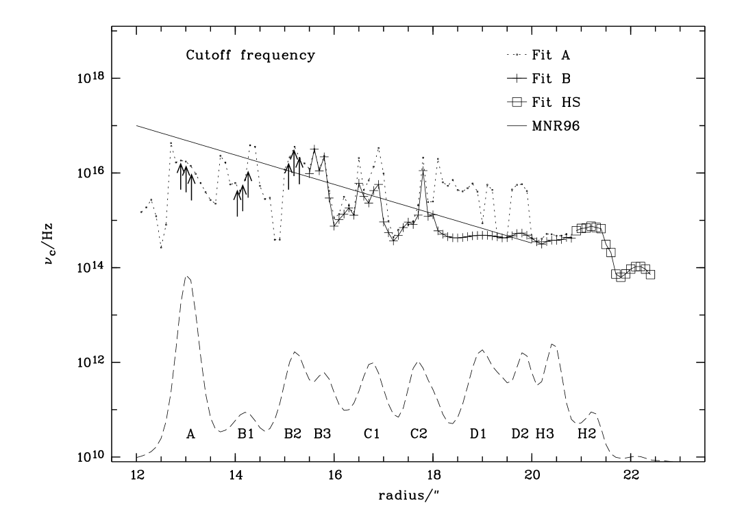
Figure 16: Run of the fitted cutoff frequency $\nu_{\mathrm{c}}$ along the jet. The thin line represents the run of the cutoff frequency at 1$\aas@@fstack{\prime\prime}$3 resolution, parameterised as $\mbox{$\nu_{\mathrm{c}}$}=10^{17}\,\mathrm{Hz}\exp(-(r-12\arcsec)/1\aas@@fstack{\prime\prime}4)$ by Meisenheimer et al. (1996a). Model A has a slightly higher $\nu_{\mathrm{c}}$ than Model B. Lower limits to the true cutoff frequency are indicated by arrows. Error bars are not shown because the errors on the fitted cutoff frequency are correlated in a complicated manner with the observational flux errors and the assumed spectral shape. Variations in the cutoff frequency are expected to be significant where the variations in the high-frequency spectral indices are significant.

We present maps of the fitted cutoff frequency $\nu_{\mathrm{c}}$ for the three different fits in Fig. 15, and its run along the radius vector at position angle 222$\aas@@fstack{\circ}$2 in Fig. 16. No cutoff is observed in the regions at $r=13\arcsec$ (A1) and at 15″ (B2) (cf. §4.2), so the fitted values there are only lower limits to the true cutoff frequency. The overall trend is a decrease in $\nu_{\mathrm{c}}$ with increasing distance from the core. The lowest value of $\nu_{\mathrm{c}}$ is reached at the hot spot, which is characterised by a sharp drop in $\nu_{\mathrm{c}}$ from $10^{15}$ Hz at 21$\aas@@fstack{\prime\prime}$2 (optical hot spot position) to $10^{14}$ Hz at $r=21\aas@@fstack{\prime\prime}6$. As expected from the overall similarity of the spectral indices determined at 0$\aas@@fstack{\prime\prime}$3 resolution and in earlier work at 1$\aas@@fstack{\prime\prime}$3 resolution (Fig. 9), the cutoff frequency determined here agrees well with the run of the cutoff frequency $\mbox{$\nu_{\mathrm{c}}$}=10^{17}\,\mathrm{Hz}\exp(-(r-12\arcsec)/1\aas@@fstack{\prime\prime}4)$ determined by Meisenheimer et al. (1996a).

All variations are rather smooth. Any sharp jumps are due to the uncertainties introduced into the fitting by the fact that there are only three high-frequency data points which cannot constrain the cutoff frequency and the UV excess well simultaneously. Therefore, only those local peaks are significant which correspond to significant peaks in the high-frequency spectral indices (Fig. 8). In fact, local peaks in the cutoff frequency are not as pronounced as expected from the peaks in the infrared-optical spectral index, e.g. at C2 and D2. Considering the fits in these locations (Fig. 12), it is apparent that the cutoff frequency is likely overestimated in those locations. In any case, there is a tendency for the cutoff frequency to be slightly higher in the brighter regions than in the immediate surroundings. However, the variation in cutoff frequency is less pronounced than the corresponding variation in the jet’s surface brightness at all wavelengths. Thus, there is a local positive correlation between brightness and cutoff frequency, while globally, the cutoff frequency decreases along the jet as the (radio) surface brightness increases.

Only small discrepancies arise in the value of the cutoff frequency between Model A and Model B for most of the jet (for a discussion, see §6.2 below). Between $r=17.5$ and $r=19.5$, where the spectral hardening is most pronounced, the value of $\nu_{\mathrm{c}}$ in Model A, in which the cutoff is determined mainly by the optical-UV spectral index, is a factor of 3–10 larger than in the preferred Model B, in which the steeper (by $\Delta\alpha\approx 0.2$) infrared-optical spectral index determines the cutoff frequency. Before we discuss the variation of the particles’ maximum energy along the jet, we consider the derived minimum-energy field.

5.4.2 The equipartition magnetic field

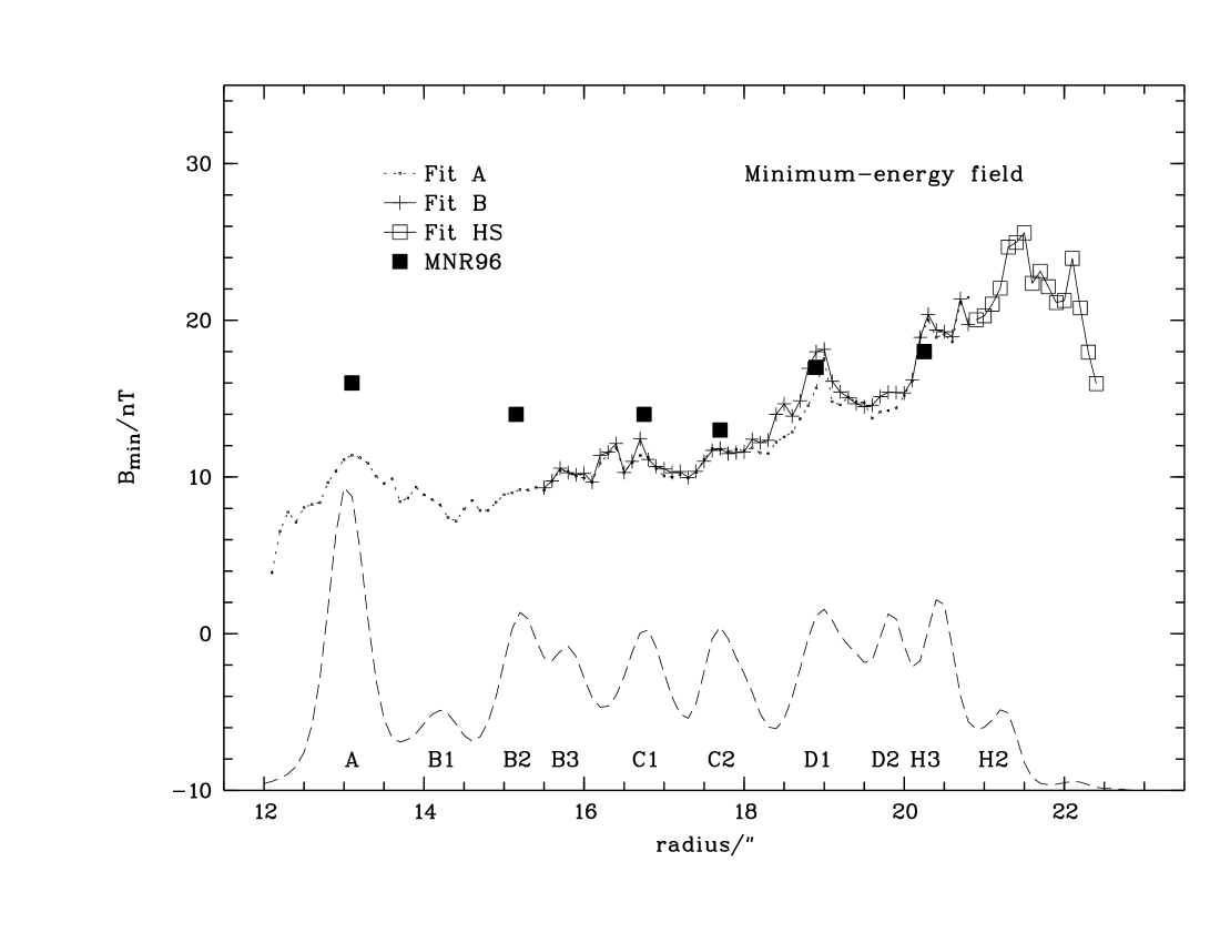
Figure 17: Run of the minimum-energy field $B_{\mathrm{min}}$ along the jet. The solid points show the values determined for individual regions by Meisenheimer et al. (1996a). The overall run corresponds to that of the jet luminosity. The most recent value for the magnetic field determined for the hot spot is $(39^{+24}_{-10})$ nT.; correcting for a different value of $k$ in Eqn. 7 brings this into agreement with the present determination. Other discrepancies are due to the different volumes assumed for the emission regions, which were modeled as individual blobs by Meisenheimer et al. (1996a).

radius/″

Figure 18: Map of the bolometric surface brightness assuming isotropic emissivity. Values range from $1.5\times 10^{34}$ W/pixel at the peak of knot A to $1.9\times 10^{35}$ W/pixel in the hot spot with a pseudo-logarithmic stretch as indicated by the greyscale bar. The hot spot has a luminosity of approximately $1.31\times 10^{37}$ W (sum of H2 and H1), which is just a little more than the total luminosity of the jet at $r\leq 20\aas@@fstack{\prime\prime}7$ of $1.26\times 10^{37}$ W. The luminosity of regions A and B2 could be much larger than indicated here if the synchrotron spectrum extends up to X-rays.

The variation of the derived minimum-energy field perpendicular to the jet axis is dominated by the assumed geometry. We therefore present only its run along the assumed jet axis in Fig. 17. It starts at just below 10 nT at the onset of the optical jet, increasing to 20–25 nT in the hot spot. The corresponding value of the electron number density ranges from about 1-5 m^-3. The evolution of the minimum-energy field along the jet corresponds qualitatively to the run of the bolometric surface brightness (Fig. 18). This is expected because for the constant spectral shape assumed here (justified by the constant radio spectral index) and for a constant emitting volume, the minimum-energy field scales with the surface brightness $S(\nu_{0})$ (at any frequency $\nu_{0}$ significantly below the cutoff frequency) as $S^{2/7}$. As already noted in §§5.2 and 5.3.2 above, the cutoff frequency has negligible influence on the minimum-energy field for spectra with $\alpha<-0.5$. Therefore, the possibility that the synchrotron spectrum extends up to X-rays in regions A, B1 and B2 has no influence on the minimum-energy estimate.

The minimum-energy field of $\approx 25$ nT determined for the hot spot seems to be low compared to the magnetic field value determined by Meisenheimer et al. (1997), both from spectral fits ($(39^{+24}_{-10})$ nT) and from the minimum-energy argument ($(35^{+8}_{-4})$ nT; cf. Fig. 17). This difference is entirely due to the different values assumed for the ratio $k$ in Eqn. 7, chosen as $k=1$ here but $k=10$ in Meisenheimer et al. (1997). Thus, our determination of the minimum-energy field agrees with previous spectral fits at lower resolution.

As discussed below, only the order of magnitude of the minimum-energy field matters in the considerations here. We therefore do not discuss its behaviour in detail.

5.4.3 The maximum particle energy $\gamma_{\mathrm{max}}$

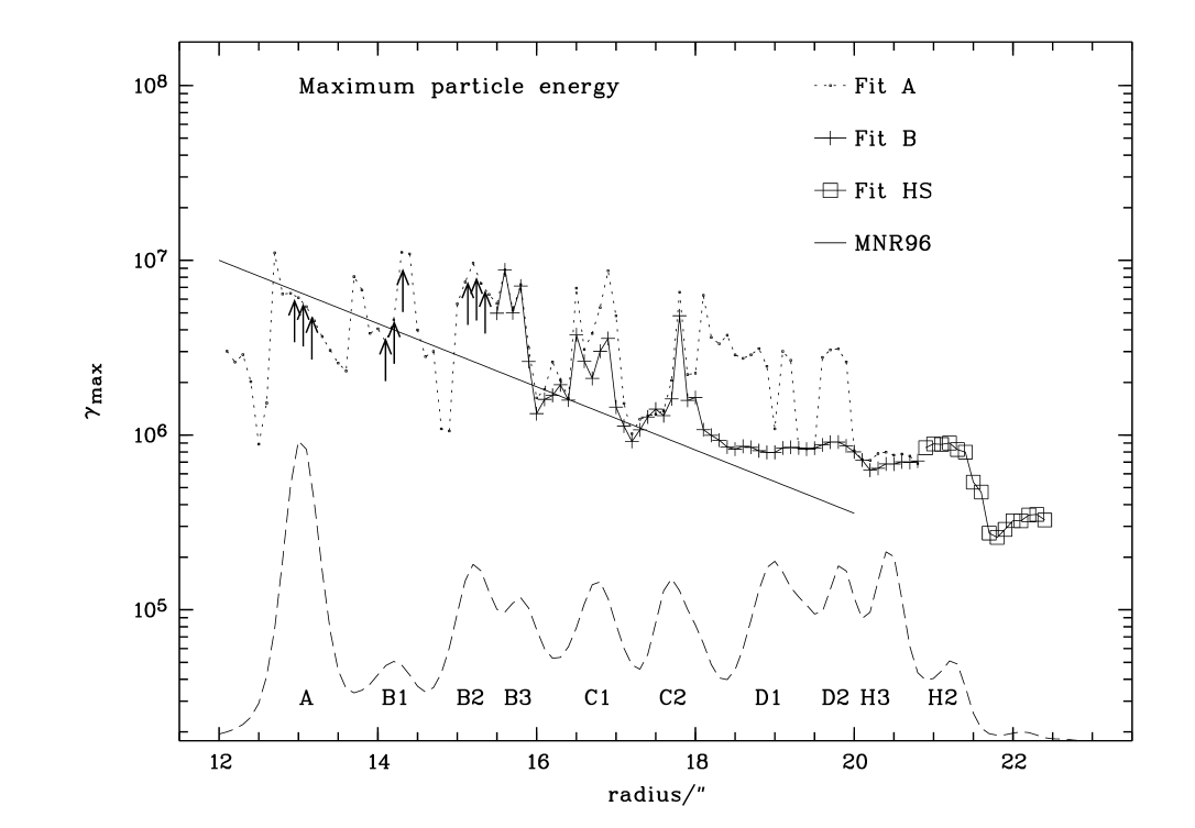
Figure 19: Run of the maximum particle Lorentz factor $\gamma_{\mathrm{max}}$ along the jet. The thin line represents the run parameterised as $\mbox{$\gamma_{\mathrm{max}}$}=10^{7}\exp(-(r-12\arcsec)/2\aas@@fstack{\prime\prime}4)$ by Meisenheimer et al. (1996a). Their points lie above our new The overall run of $\gamma_{\mathrm{max}}$ is identical to that of $\nu_{\mathrm{c}}$.

The run of the maximum particle energy inferred from the minimum-energy field and the cutoff frequency is shown in Fig. 19. This run is very similar to the run of the cutoff frequency in Fig. 16; this arises from the relation used to derive the maximum particle energy (Eqn. 1):

$$\mbox{$\gamma_{\mathrm{max}}$}=10^{7}\times\left(\frac{\mbox{$\nu_{\mathrm{c}}$}}{4.2\times 10^{15}{\rm Hz}}\right)^{\frac{1}{2}}\left(\frac{B}{\rm nT}\right)^{-\frac{1}{2}}.$$

The maximum particle energy and cutoff frequency are both plotted logarithmically, that is, we are comparing their order of magnitude. Hence, the run of the two can only differ if the order of magnitude of the magnetic field changes significantly along the jet. This is not the case, as expected from the fact that the minimum-energy field scales as $S_{\nu}^{2/7}$ (cf. §5.4.2 and Fig. 17). This implies that although the variations of $B_{\mathrm{min}}$ perpendicular to the jet axis are dominated by the assumed geometry, the variations in $\gamma_{\mathrm{max}}$ are not affected as greatly. We therefore show a map of the maximum particle energy in Fig. 20 in addition to the development of $\gamma_{\mathrm{max}}$ along the jet axis presented in Fig. 19.

image

620${\rm\thinspace\,nm}$

$\log\mbox{$\gamma_{\mathrm{max}}$}$

Model A

$\log\mbox{$\gamma_{\mathrm{max}}$}$

Model B

Figure 20: Map of the maximum particle Lorentz factor $\gamma_{\mathrm{max}}$. The results for Model HS have been inserted in both. Only in regions A and B2 does $\gamma_{\mathrm{max}}$ show a strong correlation to features of the radio-optical jet morphology. The only differences between Model A and Model B occur in regions C–H3, where the discrepancies between the infrared-optical and optical-ultraviolet spectral indices are strongest.

As expected from the run of the spectral indices from previous studies, the global trend is a decrease of $\gamma_{\mathrm{max}}$ from $>10^{7}$ down to $10^{5}$–$10^{6}$. Simultaneously, there is a strong increase of the jet’s luminosity, i. e., luminosity and maximum energy are anti-correlated. We consider the local variations next. As we noted above, local extrema of the infrared-optical spectral indices correspond to extrema of $\nu_{\mathrm{c}}$ and hence of $\gamma_{\mathrm{max}}$ because the minimum-energy field does not change much along the jet. Significant local extrema of $\gamma_{\mathrm{max}}$ are found in the following regions:

• A and B2 (13″and 15$\aas@@fstack{\prime\prime}$5), in which both high-frequency spectral indices peak simultaneously at a value significantly flatter than the radio-infrared spectral index

• C1 and C2 (16$\aas@@fstack{\prime\prime}$75 and 17$\aas@@fstack{\prime\prime}$75), where both high-frequency spectral indices show a local peak; here, the infrared-optical spectral index peaks at the brightness maximum, while the optical-UV maxima are slightly offset radially outward

• The radio hot spot H2, at which all high-frequency spectral indices and the radio-infrared index drop significantly. $\gamma_{\mathrm{max}}$ starts to drop from a value $\mbox{$\gamma_{\mathrm{max}}$}\approx 10^{6}$ at the optical counterpart to H2 and reaches a plateau beyond the radio hot spot at one-third of the pre-hot spot value. This drop corresponds to the absence of optical and ultraviolet emission beyond the radio hot spot in the tip of the jet H1. The detailed run of the cutoff frequency in the hot spot is determined not only by the spectral evolution downstream of the Mach disk, which is located at the highest-frequency emission peak, but also by the effect of telescope resolution and integrating along the line of sight through the cylindrical emission region oriented at 45°to the line of sight (Heavens & Meisenheimer 1987).

Thus, like for the cutoff frequency, the local variations of $\gamma_{\mathrm{max}}$ show the exact opposite behaviour of the global variations: in regions A and B2, there is a strong positive correlation between energy output and cutoff energy. A much weaker, but still positive correlation is observed for the remainder of the jet’s knots. Globally, however, the cutoff frequency decreases as the radio jet becomes brighter. We consider possible explanations in §6.4 below.

6 Discussion

6.1 The hot spot

Meisenheimer & Heavens (1986) presented a model for particle acceleration in the hot spot of 3C 273. They showed that the hot spot spectrum can be understood by modelling the hot spot as a planar shock at which first-order Fermi acceleration of particles takes place (details of the spectral modelling are contained in Heavens & Meisenheimer (1987), while further observations of this and other hot spots have been presented by Meisenheimer et al. (1989, 1997)). This model predicts an offset between the peaks of the radio and optical emission of 0$\aas@@fstack{\prime\prime}$2, arising from the vastly different synchrotron loss scales of electrons being advected downstream from the shock itself: “radio” electrons lose a negligible fraction of their total energy, while “optical” electrons quickly lose their entire energy as they move away from the acceleration region. Recall that the strong compression at the shock leads to an increased magnetic field compared to the jet flow, and hence to stronger losses.

Figure 5 clearly shows the predicted offset in the position of the hot spot (H2) between radio and optical wavelengths. This strengthens the identification of H2 with a planar shock with strongly localised particle acceleration.

We note that again the minimum-energy magnetic field determined for the hot spot agrees with the magnetic field determined from the hot spot spectrum by Meisenheimer et al. (1997, the only difference arises due to different values of the parameter $k$ in the minimum-energy field determination).

Thus, at 0$\aas@@fstack{\prime\prime}$3 resolution, the Heavens & Meisenheimer (1987) hot spot model is consistent with all observations. Moreover, our new observations have confirmed the predicted offset in the hot spot’s position. However, it is remarkable that even the hot spot shows a UV excess, indicating that the hot spot, too, has a more complicated internal structure than previously assumed. In addition, the presence of emission from the tip of the jet H1 (which has been called a “precursor” in the literature; see Foley & Davis 1985, e.g.) and its relation to the hot spot must be explained. The next tests of this model will involve a detailed analysis of the hot spot’s radio morphology at the highest available resolution, which we defer to a future paper.

6.2 Flatter spectra at higher frequencies: the need for a second emission component

When describing synchrotron spectra as power laws, the underlying assumption is a power-law electron energy distribution. As noted above, a non-idealised spectrum with finite maximum particle energy and rapid pitch-angle scattering will furthermore exhibit a quasi-exponential cutoff at some frequency $\nu_{\mathrm{c}}$, the synchrotron frequency corresponding to the highest electron energies. This cutoff implies that the spectrum has a convex shape, so that the spectrum steepens progressively towards higher frequencies. Any high-frequency flux must therefore lie below a power-law extrapolation from lower frequencies.

In employing broken power laws, the only physical break is a steepening of the spectrum from $|\alpha_{\mathrm{low}}|$ to $|\alpha_{\mathrm{high}}|=|\alpha_{\mathrm{low}}|+1/2$ near some break frequency $\mbox{$\nu_{\mathrm{b}}$}<\mbox{$\nu_{\mathrm{c}}$}$. This break arises in a model of the synchrotron source as a loss region into which a power-law distribution of electrons with approximately constant number density and maximum energy is continuously injected. The break is produced by adding up the contributions from the electron population observed at different times since acceleration, i. e., with different cutoff frequencies. The magnitude of the break of $1/2$ is fixed by the cooling mechanism. Describing synchrotron spectra with arbitrary breaks is therefore inconsistent with any physically motivated model; in violation of our reasoning above, one could then even invent breaks to flatter spectra.

We used the detailed shape of cutoff spectra as computed by Heavens & Meisenheimer (1987). The spectral shape is the result of observing a mixture of electron populations, and the appearance of the entire source can be understood in terms of the temporal evolution of the initially accelerated population. As long as the spectral shape is determined only by radiation losses, not even homogeneous source conditions are required. The resulting spectrum rarely will follow a power law over many decades in frequency, but will be curved and in any case exhibit a convex shape.

In contrast, a more complex electron distribution could be produced if different parts of a source accelerate electrons to different maximum energies, and contain different numbers of electrons. Such a source could be a jet with an inhomogeneous distribution of particles and magnetic fields. This source must be described by more than one electron population (or equivalently, as the sum of the emission from more than one source). This corresponds precisely to the situation encountered in 3C 273’s jet: the observed flattening of the spectrum implies that a description using a single electron population is inadequate. This implies unambiguously that there are at least two components to the observed spectrum: one is the “low-frequency” synchrotron spectrum from radio through optical wavelengths. In addition, there is a “high-frequency” component responsible for the UV excess, and hence the observed flattening. We have suggested that this second component is the same as that responsible for the jet’s X-rays (Jester et al. 2002), which could be a second synchrotron component (Röser et al. 2000; Marshall et al. 2001) or beamed inverse Compton emission (cf.  Sambruna et al. 2001) . In any case, our spectra prove that 3C 273’s jet is not a homogeneous synchrotron source.

It is notable that besides 3C 273, the spectral energy distributions (SEDs) of M87’s jet shows the same upward curvature: Marshall et al. (2002) have presented SEDs for that jet from radio through X-rays (their Fig. 3). They fitted two different single-population models, a Jaffe-Perola model assuming a randomly tangled magnetic field structure and pitch-angle scattering, and a Kardashev-Pacholczyk model, also assuming a tangled field but no pitch angle scattering. Only the latter provides an acceptable fit to the observed SEDs, but it is unclear how pitch-angle scattering could be avoided in a tangled field geometry. Moreover, the spectra for knots HST-1 and D clearly show a steeper downturn near $10^{15}$ Hz (already hinted at by the ground-based spectra obtained by Meisenheimer et al. 1996b, their Figs. 7 and 8) than the Kardashev-Pacholczyk spectrum, which is therefore inadequate. Instead, again a second spectral component must be invoked to account for the X-ray flux lying above the cutoff observed in the near-infrared–optical region. Marshall et al. (2002) viewed this as evidence in favour of the spatially stratified model for M87’s jet presented by Perlman et al. (1999).

6.3 Slow decline and smooth changes in $\gamma_{\mathrm{max}}$: the need for an extended acceleration mechanism

Our determination of the maximum energy of synchrotron-emitting electrons shows a lower limit for the Lorentz factors of $\mbox{$\gamma_{\mathrm{max}}$}>10^{7}$ at the onset of the optical jet, 12″ from the quasar core (Fig. 19). The maximum Lorentz factor first drops outward along the jet, and then stays nearly constant at a Lorentz factor of a few times $10^{6}$ at radii $>17\arcsec$. It drops again by factor of 3 within the hot spot. This drop most likely is caused by the stronger magnetic field there. In any case, the Lorentz factor of the particles emitting optical synchrotron radiation cannot be much lower than $10^{5}$ anywhere in the jet. Electrons with such high energies can only be observed close to their acceleration sites: as noted in all previous studies, synchrotron cooling timescales for these particles are of the order of a few hundred or thousand years (see Guthrie & Napier 1975; Röser & Meisenheimer 1991; Meisenheimer et al. 1996a, e.g.). The corresponding loss scales are a few hundred parsec for the case of electrons freely streaming at the speed of light, which is unrealistic since they will have to follow tangled field lines.

The development of the maximum particle energy along the jet is therefore consistent with the absence of any synchrotron cooling. The same conclusion can already be drawn from the smooth changes of just the optical spectral index, which should most strongly reflect the synchrotron losses the particles undergo, and from the mere presence of optical synchrotron radiation along the entire jet (Jester et al. 2001). The apparent absence of cooling in the presence of synchrotron radiation can only be explained by a distributed acceleration mechanism.

The smooth changes of the spectral features along the jet indicate a correspondingly smooth variation of the physical conditions along the jet. The present detailed high-resolution study of the jet in 3C 273 set out with the aim to map those regions in which particles are preferentially accelerated. Since the observed cooling is much less drastic than expected, the conclusion is that the entire jet is the particle acceleration region. The fact that the jet has a much higher emissivity than the radio cocoon around it (see §4.1.3) also implies a difference in physical conditions between the jet and the surrounding material. Furthermore, the jet’s X-ray emission is a further sink of energy (whatever the emission process) which needs to be filled by the re-acceleration mechanism. Note that this does not preclude the possibility that the knots in the jet are due to shocks, at which particle acceleration can also take place. But even in this case, particles must be accelerated between the shocks as well.

This corresponds to the “jet-like” acceleration mechanism proposed by Meisenheimer et al. (1997). The detailed physics of this distributed acceleration mechanisms are unknown, but several theoretical suggestions have been made. Magnetic reconnection is one way to tap the energy stored in the jet fluid and convert it continuously into relativistic particles (Litvinenko 1999). Another possible energy source is the velocity shear between the surface of the jet and the surrounding medium (Stawarz & Ostrowski 2002). This latter mechanism would be limited to particle acceleration within a thin surface layer. Since it appears that the jet emission is not edge-brightened, as would be expected for emission from a surface layer (§4.1.2), surface velocity shear is unlikely to be the acceleration mechanism providing optical electrons along the entire jet. It may, however, be appropriate to explain the second higher-energy emission component identified above (§6.2), provided this turns out to be edge-brightened. A similar mechanism has recently been proposed by Rieger & Mannheim (2002): these authors suggest that velocity shear and centrifugal forces in a rotating jet flow may provide efficient particle acceleration.

The global energy budget of the jet is a related question. If the entire jet operates at the minimum energy condition, and if there is no strong, variable beaming, the increase in the minimum-energy field along the jet (linked to the increase in synchrotron luminosity) corresponds to an increase of the energy density stored in magnetic fields and relativistic particles by about one order of magnitude. This raises interesting questions about the energy budget of the jet: If the total energy flux in magnetic fields and relativistic particles is to be conserved, the jet would need to slow down (cf.  Georganopoulos & Kazanas 2003). The necessity to account for the kinetic energy and momentum flux imposes further constraints. On the other hand, it may be possible to convert jet kinetic energy into magnetic and particle energy, as in some of the acceleration mechanisms just mentioned, leading to a different mutual dependence of jet speed and magnetic energy density than in the pure energy conservation case. A detailed examination of the jet’s energy budget addressing these issues is certainly a worthy exercise, but beyond the scope of the present publication.

6.4 Correlations between brightness and maximum particle energy

As described in §5.4.3, there is a local positive correlation between surface brightness and maximum particle energy, although these quantities are anti-correlated globally. The opposite correlations must be caused by two different physical mechanisms. Although the cutoff frequency is the direct observable, the underlying physical parameters are the maximum particle energy and the jet’s magnetic field. In 3C 273, the global run of the maximum particle energy is practically identical to that of the cutoff frequency, and the local variations in cutoff frequency are much smaller than those in surface brightness (see Figs. 16 and 19).

We have established above (§6.3) that particles must be accelerated continuously within the jet. In this case, the value of the maximum particle energy is obtained by equating the acceleration timescale $\tau_{\mathrm{acc}}$, which is the time during which a particle’s energy is increased by a factor of two, with the synchrotron loss timescale $\tau_{\mathrm{syn}}$ (e. g., Longair 1994):

$$\tau_{\mathrm{acc}} = \tau_{\mathrm{syn}}(\gamma_{\mathrm{max}})\propto\frac{1}{B^{2}\gamma_{\mathrm{max}}}$$

$$\Leftrightarrow\gamma_{\mathrm{max}} \propto \frac{1}{B^{2}\tau_{\mathrm{acc}}}.$$ (9)

The acceleration timescale is energy-independent both for diffusive shock acceleration (e. g., Bell 1978) and for acceleration by reconnection (e. g., Litvinenko 1999). Thus, the behaviour of the maximum particle energy as a function of magnetic field depends critically on the nature of the acceleration mechanism, in particular the scaling of the acceleration time scale with the magnetic field strength.

We have taken the jet Doppler factor to be $\mathcal{D}=1$ in all calculations up to here, which is justified because the value of the maximum particle energy as inferred from the jet’s surface brightness and minimum-energy magnetic field only depends very weakly on the true value of the Doppler factor (cf. §5.2 and Neumann 1995; Meisenheimer et al. 1996a). The observed surface brightness $S$ and cutoff frequency $\nu_{\mathrm{c}}$ have the following scalings with $B$ and $\mathcal{D}$ for a continuous jet (see Begelman et al. 1984, e.g.):

$$S \propto B^{1-\alpha}\,\mathcal{D}^{2-\alpha}$$ (10)

$$\nu_{\mathrm{c}} \propto B\,\gamma_{\mathrm{max}}^{2}\,\mathcal{D}.$$ (11)

In the following discussion, we will not use the minimum-energy magnetic field, because its computation has introduced correlations between the magnetic field strength, the electron number density, and the surface brightness by construction.

6.4.1 Local correlation between brightness and maximum particle energy

The only other jet which has been studied similarly well is that in M87. There are key differences between the behaviour of the maximum particle energy between these two jets. Meisenheimer et al. (1996b) showed that M87 shows a strong correlation between surface brightness and cutoff frequency, while the maximum particle energy remains practically unchanged. This correlation can be understood purely in terms of variations of the magnetic field strength, while the constancy of the maximum particle energy is explained by invoking acceleration in shocks (e. g. Sparks et al. 1996), by an extended acceleration mechanism (Meisenheimer et al. 1996b), or by assuming a sub-equipartition magnetic field and relativistic time dilation which both lower the loss times sufficiently even without particle acceleration (Heinz & Begelman 1997). Meisenheimer et al. (1996b) conclude that re-acceleration is responsible, and that the mechanism in M87’s jet obeys the scaling $\tau_{\mathrm{acc}}\propto B^{-2}$ to achieve a constant maximum particle energy (cf. Eqn. 9). It is useful to consider whether this acceleration mechanism proposed for M87 could be identical to the one at work in 3C 273, i. e., whether it is universal.

Since the maximum particle energy changes significantly along 3C 273’s jet, the acceleration mechanism invoked by Meisenheimer et al. (1996b) for M87 must be different from the one acting in 3C 273’s jet. To produce a local correlation between brightness and maximum particle energy via magnetic field variations, the acceleration time scale in 3C 273 would need to follow a scaling $\tau_{\mathrm{acc}}\propto B^{s}$ with $s>2$ so that both $\gamma_{\mathrm{max}}$ and $S$ correlate with $B$ (Eqns. 9 and 10). In that case, local magnetic field variations could explain the observed correlations. However, since the brightness changes are larger than the changes in the maximum particle energy and cutoff frequency, it seems more likely that small-scale variations in the Doppler factor $\mathcal{D}$ are responsible because $S$ varies more strongly with $\mathcal{D}$ than with $B$. But variations in $\mathcal{D}$ by themselves are insufficient for 3C 273 because they do not produce a correlation between brightness and maximum particle energy. To clarify the origin of this correlation, it will be necessary to disentangle the UV excess from the remainder of the jet emission to remove any uncertainty about the true value of the cutoff frequency, and ideally to obtain a measurement of the jet’s magnetic field other than the minimum-energy estimate.

6.4.2 Global anti-correlation of brightness and maximum particle energy

The global anti-correlation of brightness and maximum energy appears intuitive for synchrotron radiation: stronger synchrotron emission implies larger energy losses, and hence a lower maximum energy. However, as noted above, the actual behaviour of the maximum particle energy in the presence of particle acceleration depends on the details of the acceleration mechanism. If the local correlation of brightness and $\gamma_{\mathrm{max}}$ can be explained by the nature of the acceleration mechanism, the global anticorrelation must be due to an entirely different effect which reverses the local correlation. It may be possible that the local correlations are produced by a “shock-like” acceleration mechanism acting only in the brighter regions (e. g.if the bright regions are shocks), while electrons elsewhere are accelerated by the “jet-like” mechanism (Meisenheimer et al. 1997). However, such a scenario is somewhat unappealing because there would need to be a certain fine-tuning to explain the overall smoothness of the spectral index changes. Furthermore, although this may explain the different global and local behaviour within 3C 273 as well as the presence of two distinct emission components (§6.2), the difference to M87 remains, in which the “jet-like” mechanism is assumed to produce the positive correlation. We therefore need to appeal to further differences. Meisenheimer (1996) suggested that the observations of M87 and 3C 273 could be unified if there was a link between the maximum particle energy and the velocity gradient along the jet, and the jet velocity was relativistic, so that changes in the velocity would lead both to changes in the maximum particle energy and in the Doppler factor and hence the apparent brightness. We will discuss this idea elsewhere.

7 Summary and future work

One of the main unsolved questions in the study of extragalactic jets is posed by the observations of optical synchrotron radiation over scales much larger than typical synchrotron loss scales and far from the “working surfaces” of the standard model (Blandford & Rees 1974). Another puzzle has been posed by the recent Chandra observations of X-rays from extragalactic jets, whose emission mechanism remains debated and which form a further sink of energy that has to be filled within the jet. The study of the physical conditions giving rise to the observed emission by keeping up the particle energy against strong synchrotron losses at optical wavelength and supplying the energy observed in X-rays can only be performed via a study of the synchrotron continuum, at the highest possible spatial resolution and covering the largest possible wavelength range.

7.1 Observations

We present new HST and VLA images of the jet at $\lambda\lambda$ 3.6${\rm\thinspace cm}$, 2.0${\rm\thinspace cm}$, 1.3${\rm\thinspace cm}$, 1.6 $\mu$m, 620${\rm\thinspace\,nm}$ and 300${\rm\thinspace\,nm}$ matched to a common resolution of 0$\aas@@fstack{\prime\prime}$3 (Fig. 2). We combine the data to obtain spectral energy distributions which we fit with theoretical synchrotron spectra (Fig. 12). Contrary to expectations for synchrotron emission, the observed spectra show a significant flattening in the infrared-ultraviolet wavelength range, implying that the emission cannot be modelled as synchrotron emission due to a single electron population, as has been assumed in previous studies of this jet’s emission (Meisenheimer et al. 1996a). Instead, additional emission must be present which can lead to the observed flattening. The most likely explanation is an additional flat-spectrum component in the ultraviolet. The same component may simultaneously be responsible for the jet’s X-ray emission (for details, see Jester et al. 2002).

The optical-ultraviolet spectral index map generated at 0$\aas@@fstack{\prime\prime}$3 resolution (Fig. 7a) shows no strong correlation between local spectral index and surface brightness variations. There is, however, such a correlation on the radio-infrared and infrared-optical spectral index maps. Even these correlations are less pronounced than those found in the jet of M87 (Perlman et al. 2001, 2002), where they are taken as evidence of localised particle acceleration in the knots of this jet (but see Meisenheimer 1996 for an alternative explanation). As confirmed by our spectral fits (see below), the spectral index variations reflect variations of the maximum particle energy along the jet.

We find an offset between the radio and optical images of the hotspot that is consistent with the prediction by Heavens & Meisenheimer (1987). This adds further to the confidence that the assumed hot spot model is correct (Meisenheimer et al. 1997). However, the role of the tip of the jet H1 and its relation to the hot spot remains to be clarified, perhaps in a model fully describing the hot spot flow in three dimensions, instead of just one. If the jet flow is still highly relativistic just upstream of the hot spot, the details of the flow’s deceleration in the hot spot may also change its appearance (Georganopoulos & Kazanas 2003).

7.2 Synchrotron spectral fits

We fitted the observed spectra with model synchrotron spectra to extract physical information, in particular the maximum particle energy and its variation along the jet.

Model synchrotron spectra according to Heavens & Meisenheimer (1987) have been used to determine the cutoff frequency $\nu_{\mathrm{c}}$. It is mainly determined by the infrared-optical spectral index. We infer the maximum particle energy from the fitted cutoff frequency by assuming an equipartition magnetic field $B_{\mathrm{min}}$. It is a general result that the value of $B_{\mathrm{min}}$ is very robust with respect to assumptions about the details of the spectral shape, as long as the spectrum has a power law index that is steeper than $\alpha=-0.5$.

The cutoff frequency decreases from above $5\times 10^{6}$ in region A at $r\approx 13\arcsec$ and settles to a plateau of order $10^{6}$ at $r\ga 18\arcsec$. A further decrease to $\mbox{$\gamma_{\mathrm{max}}$}\approx 3\times 10^{5}$ is only observed at the position of the radio hot spot, beyond which there is no optical, but still infrared emission. This global run corresponds to the findings of previous studies at 1$\aas@@fstack{\prime\prime}$3 resolution, which showed that the maximum particle energy decreases as the radio jet brightness increases. As expected from the spectral index variations, there is an additional weak correlation between local variations of maximum particle energy and surface brightness.

An earlier examination of the effect of relativistic beaming on the inferred synchrotron lifetime had shown that the overall slow decrease of $\gamma_{\mathrm{max}}$ cannot be explained by an enhancement of the true synchrotron lifetime by beaming effects (Jester et al. 2001). We concluded that particle acceleration must take place distributed across the entire jet. This conclusion is strengthened by the X-ray observations, whatever the X-ray emission mechanism: The radiative lifetimes of X-ray synchrotron electrons in an equipartition field of 20 nT are a few tens of years, those of UV-emitting electrons are a few hundreds of years. In the inverse Compton scenario, the combined effects of relativistic beaming and lower magnetic fields lead to lifetimes of a few times $10^{4}$ years for UV-emitting electrons. In both cases, particles must therefore be accelerated continuously within the entire jet (“jet-like” acceleration, Meisenheimer et al. 1997). The same conclusion is drawn from the fact that the physical conditions within the jet of 3C 273 vary very smoothly down to the spatial scales of $0.9h_{70}^{-1}\mbox{${\rm\thinspace kpc}$}$ resolved here. This does not preclude the possibility that the enhanced-brightness regions are shocks at which particles are accelerated – but even if they are, re-acceleration between them is necessary to explain the observed spectral features.

The details of the acceleration mechanism determine the scaling of the maximum particle energy with changes in the magnetic field. The interplay between the “jet-like” and “shock-like” acceleration mechanisms might explain the conflicting global and local behaviour of the maximum particle energy in 3C 273. However, both mechanisms must be different from the one invoked by Meisenheimer et al. (1996b) for M87’s jet (§6.4).

We stress again the observed flattening of the high-frequency spectrum, which implies that the jet’s emission cannot be assumed to arise from a single electron population, but requires the presence of an additional emission component. In particular, the spectrum of knot A cannot be considered as a single power law from radio through X-rays, as concluded from lower-resolution data (Röser et al. 2000; Marshall et al. 2001). Instead of considering the jet as a homogeneous synchrotron source filled with a simple electron population, we must realise that jets have an internal energetic structure (cf. Perlman et al. 1999, 2001). Future work to investigate the acceleration mechanism at work in this and other jets must be based on these results.

7.3 Future work

With the present radio-optical data, it has only been possible to detect the high-frequency hardening of the jet emission, and thus the presence of a second emission component. No statements can be made about the spectral shape of this “high-energy” component beyond the approximate match of the X-ray extrapolation and the UV excess. We have been awarded HST time to extend the wavelength coverage into the far-ultraviolet (150 nm). Using these data, we will be able to constrain the run of the optical synchrotron cutoff more accurately, and to characterise the spectrum of the UV excess. This will achieve a separation of the two spectral components from each other. Particular insight can be expected by considering the high-frequency spectra in those regions of the jet showing the strongest difference between radio, optical and X-ray morphology (§4.1.1).

In order to test theories for extended particle acceleration, we require detailed predictions both from theoretical work and from magneto-hydrodynamical simulations of the jet flow, in particular regarding the spatial distribution of relativistic particles. The most sensitive observational tool is multi-wavelength polarimetry resolving the jet width. This allows not only a study the particles’ energy distribution, but also an assessment whether particles at different energies probe the same underlying magnetic field, that is, whether they actually occupy the same emitting volume. Thus, multi-wavelength polarimetry is the natural followup programme for our detection of multiple emission components. We will use our guaranteed time for the adaptive optics camera CONICA/NAOS at the VLT to obtain near-infrared polarimetry at a resolution comparable to the data presented here. However, optical polarimetry of 3C 273’s jet making full use of the HST’s capabilities is still missing.

Exciting new facts about the jet in 3C 273 have been revealed by each advance in optical and radio observing technology. From the surprising observational facts encountered here, more surprises are yet to be expected en route to an understanding of the physics of this object. Current advances in numerical work are also expected to shed further light on the structure and dynamics of jets. As an extreme object of its kind, 3C 273 will remain high on the agenda of astrophysicists studying jet phenomena.