Jet velocity in SS433: its anti-correlation with precession-cone angle and dependence on orbital phase

Abstract

We present a re-analysis of the optical spectroscopic data on SS 433 from the last quarter-century and demonstrate that these data alone contain systematic and identifiable deviations from the traditional kinematic model for the jets: variations in speed, which agree with our analysis of recent radio data; in precession-cone angle and in phase. We present a simple technique for separating out the jet speed from the angular properties of the jet axis, assuming only that the jets are symmetric. With this technique, the archival optical data reveal that the variations in jet speed and in precession-cone angle are anti-correlated in the sense that when faster jet bolides are ejected the cone opening angle is smaller. We also find speed oscillations as a function of orbital phase.

1 Introduction

In a recent paper (Blundell & Bowler, 2004) we presented the deepest yet radio image of SS 433, which revealed an historical record over two complete precession periods of the geometry of the jets. Detailed analysis of this image revealed systematic deviations from the standard kinematic model (Margon, 1984; Eikenberry et al, 2001). Variations in jet speed, lasting for as long as tens of days, were needed to match the detailed structure of each jet. Remarkably, these variations in speed were equal, matching the two jets simultaneously.

The Doppler residuals to the kinematic model show little variation with the precessional phase of the jets and this observation rules out variations in jet speed alone as the source of the residuals (e.g.  Katz & Piran, 1982; Eikenberry et al, 2001). Very little phase variation is obtained if the pointing angle jitters (Katz & Piran, 1982) but there is no evidence excluding symmetric speed variations of the magnitude reported in Blundell & Bowler (2004) superposed on pointing jitter, Fig 1. Thus our findings from the radio image led us to re-analyse the archival optical data. G. Collins II and S. Eikenberry (with kind permission of B. Margon) made available their compiled datasets, published in Collins & Scher (2000) and used in Eikenberry et al (2001). We use the Collins’ compilation (available at http://www-astro.physics.ox.ac.uk/$\sim$kmb/ss433/) because of its higher quoted precision, but very similar results are obtained from Margon’s.

2 Speed and angular variations from the optical data

If the precessing jet axis of SS 433 traces out a cone of semi-angle $\theta$ about a line which is oriented at an angle $i$ to our line-of-sight with jet velocity $\beta$ in units of $c$ ($\gamma=(1-\beta^{2})^{-1/2}$), the redshifts measured from the west jet ($z_{+}$) and the east jet ($z_{-}$) are given, if the jets are symmetric, by:

$$z_{\pm}=-1+\gamma[1\pm\beta\sin{\theta}\sin{i}\cos{\phi}\pm\beta\cos{\theta}\cos{i}],$$ (1)

where $\phi$ is the phase of the precession cycle (see http://www-astro.physics.ox.ac.uk/$\sim$kmb/ss433/). Addition of $z_{+}$ and $z_{-}$ in Eqn 1 gives an expression relating the observed redshifts to the jet speed independently of any angular variation. Re-arrangement gives

$$\beta=\left[1-\left[1+\frac{z_{+}+z_{-}}{2}\right]^{-2}\right]^{1/2}.$$ (2)

The quantity $z_{+}+z_{-}$ fluctuates very substantially (see Fig 2). Subtraction of the expressions for $z_{+}$ and $z_{-}$ gives the angular properties $a$ of the orientation of the jet axis, with the speed divided out using Eqn 2:

$$a=\frac{z_{+}-z_{-}}{2\beta\gamma}=\sin{\theta}\sin{i}\cos{\phi}+\cos{\theta}\cos{i},$$ (3)

Fluctuations in $\beta$, $\theta$ and $\phi$ are predominantly symmetric, as described by Eqns 1–3, when fluctuations in $z_{+}+z_{-}$ represent symmetric fluctuations in speed. (The velocity variations in the two radio jets (Blundell & Bowler, 2004) are highly symmetric; the standard deviation on the difference in the speeds is less than $0.004\,c$ and on the common velocity $0.014\,c$.)

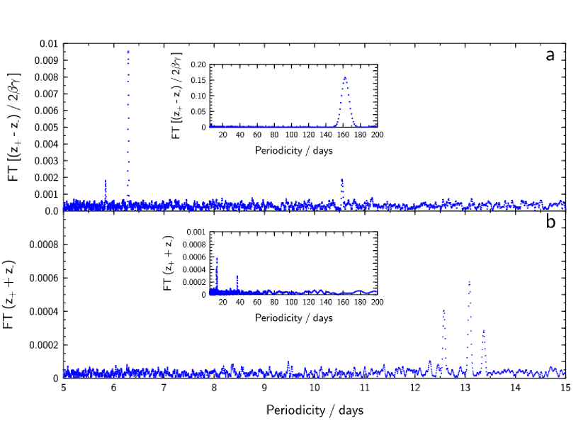
Figure 3: Fourier transform of data as described in § 2. (a) The differences of all redshift pairs, divided by $2\beta\gamma$ (see Eqn 3) which, if the jets are symmetric, depend only on the angular properties of the jet. (b) The sums of all redshift pairs which, if the jets are symmetric, only depend on the speed of the jet.

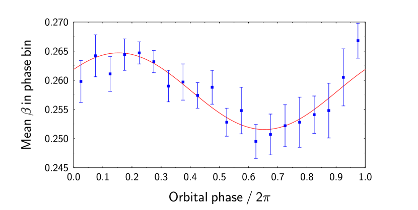
Figure 4: Speed data (Eqn 2) folded over the orbital period of 13.08 days showing a clear sinusoid, mean $0.2581\pm 0.0005$, amplitude $0.0066\pm 0.0007$, phase offset with respect to optical ephemeris $2.17\pm 0.11$ rad.

The disadvantages of the variables $s=z_{+}+z_{-}$ and $a$ (Eqn 3) are that their interpretation is simple only for perfect symmetry and that they may only be used for the 395 out of 486 observations which record a simultaneous pair. Their merits are exemplified by Fourier analyses of the time distributions. We used the algorithm of Roberts et al (1987) which accounts for the uneven time-sampling of the data. The angular data $a$ clearly revealed periodicities corresponding to the nodding of the precession axis (Katz et al, 1982; Newsom & Collins, 1982; Collins & Scher, 2002) and the 162-day precession period, clearly seen in Fig 3a. There is no periodicity in the speed data $s$ (Fig 3b) common to the angular data, consistent with perfect symmetry. The speed data also indicate a periodicity at 13.08 days (the periodicity at 12.58 days matches a beat with Earth’s orbital period 365 days); to investigate this, we folded the data over 13.08 days in 20 phase bins, and in each bin the mean speed ($\beta$, from Eqn 2) was derived. Fig 4 shows a clear sinusoidal oscillation with orbital phase. The rms variation in speed which oscillates with orbital phase is smaller by a factor of three than the overall speed dispersion. This oscillation with amplitude $2000\,{\rm km\,s^{-1}}$ may be because the speed with which the bolides are ejected is a function of orbital phase, but the excursions in Fig 4 could also be interpreted as due to orbital motion; in that case SS 433’s orbital speed is $\sim 400\,{\rm km\,s}^{-1}$.

3 Anti-correlated deviations in jet speed and $\theta$

We fitted Collins’ dataset with the kinematic model, including nodding. From our fit, we derived model redshift pairs and hence the variables $s$ and $a$. Subtraction of these model variables from those constructed from the data gave residuals $\Delta s$ in $s$ and $\Delta a$ in $a$. The $\beta$ variation is shown in Fig 2c. The standard deviation of this histogram is 0.013, in excellent agreement with the result from our radio image (0.014). Examples of the residuals in $s$ and in the angular variable $a$ are plotted in Fig 2; the variations in speed and angular residuals are anti-correlated. From Eqns 1–3, maintaining the assumption of symmetry:

$$\Delta s^{2}=4\beta^{2}\gamma^{6}\Delta\beta^{2},$$ (4)

$$\Delta a^{2} = (\cos\theta\sin{i}\cos\phi-\sin\theta\cos{i})^{2}\Delta\theta^{2}+(\sin\theta\sin{i}\sin\phi)^{2}\Delta\phi^{2}$$

$$- 2\sin\theta\sin{i}\sin\phi(\cos\theta\sin{i}\cos\phi-\sin\theta\cos{i})\Delta\theta\Delta\phi,$$

$$\Delta a\,\Delta s = 2\beta\gamma^{3}[(\cos\theta\sin{i}\cos\phi-\sin\theta\cos{i})\Delta\beta\,\Delta\theta$$

$$- \sin\theta\sin{i}\sin\phi\Delta\beta\Delta\phi],$$

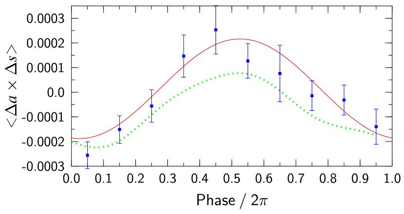
Figure 5: The mean value of $\langle\Delta a\times\Delta s\rangle$ in 162-day period phase bins, showing the best fit to Eqn 3 averaged. There are two free parameters in the fit shown as a solid line, $\langle\Delta\beta\,\Delta\theta\rangle$ and $\langle\Delta\beta\,\Delta\phi\rangle$. The dotted line shows the fit with fixed velocity but angular asymmetry.

where $\Delta\beta$, $\Delta\theta$ and $\Delta\phi$ represent the variations in $\beta$, $\theta$ and $\phi$ respectively. Averaging over many cycles for any given value of the phase $\phi$ yields the averages $\langle\Delta a^{2}\rangle$, $\langle\Delta s^{2}\rangle$, $\langle\Delta a\Delta s\rangle$ as functions of $\phi$, in terms of the parameters $\langle\Delta\beta^{2}\rangle$, $\langle\Delta\theta^{2}\rangle$, $\langle\Delta\beta\,\Delta\theta\rangle$ and so on. The fit to $\langle\Delta\beta\,\Delta\theta\rangle$ is shown in Fig 5. The parameters are given in Table 1; the global $\chi^{2}/NDF$ is 34.8/24, where $NDF$ is the number of degrees of freedom.

Fig 5 shows that the quantity $\langle\Delta a\,\Delta s\rangle$ has an almost pure cosinusoidal variation with phase, as given by the first term on the right hand side of Eqn 3. This shape is the unique signature of a correlation between variations in $\beta$ and $\theta$. $\langle\Delta\beta^{2}\rangle$ shows no correlation with $\phi$ and $\langle\Delta a^{2}\rangle$ very little. The latter requires fluctuations in both $\theta$ and in $\phi$. We remark that $\langle\Delta(z_{+}-z_{-})\,\Delta s\rangle$ does not show a strong correlation with $\phi$; nor should it, using the parameters from Table 1. Removing the varying speed from $z_{+}-z_{-}$ was crucial in revealing this correlation in $\langle\Delta a\,\Delta s\rangle$.

4 The redshift residual plot

Consider the plane of redshift residuals, as in figure 5 of Eikenberry et al (2001), with symmetric excursions from the kinematic model in $\beta$, $\theta$ and $\phi$. Comparison of their figure 5 (similar to our Fig 6f) with our Figs 6a and 6b requires the presence of both angular variations (to spread the points along the line $y=-x$) and velocity variations (to spread the points perpendicular to this line — note that even their quoted redshift measurement error of 0.003, likely an over-estimate, will not account for this breadth). Inclusion of all these variations, correlated as in Table 1, gives Fig 6d which resembles that from the data (Fig 6f). The simulations in Fig 6d take no account of the (stochastic) duration of the excursions; the duration of variations in Fig 6e were drawn from a gaussian with half-width 2 days.

Thus Figs 1 and 6 establish the consistency of the optical data with perfect symmetry and with speed fluctuations whose magnitude is in excellent agreement with those found in the radio image. In addition, the slope of Fig 6e is $-0.765\pm 0.034$, and that for Fig 6f from the Collins data set is $-0.786$ and not $-1$; this long standing curiosity is explained by the physics from the § 3 fit.

5 Other assumptions

If the jet speed were constant, the residuals to $z_{+}$ and $z_{-}$ would, for the case of strictly antiparallel jets, be correlated as in Fig 6a; to spread the distribution of points perpendicular to this line it is necessary to allow some independence in the pointing of the two jets. The variation with precessional phase of the quantities $\langle\Delta s^{2}\rangle$, $\langle\Delta a^{2}\rangle$ and $\langle\Delta a\Delta s\rangle$ is then almost as well described ($\chi^{2}/NDF=36.3/24$) as by our fit of § 3. Such a model would not be able to explain the radio jet morphology (Blundell & Bowler, 2004) and this fit required angular fluctuations breaking symmetry to have rms values $\sim 1/2$ of those preserving symmetry. Angular jitter alone cannot account for the slope of $\Delta z_{-}$ versus $\Delta z_{+}$ (Fig 6) differing from $-1$, unless the jitter in the East jet is systematically smaller than in the West jet. Velocity variation breaks symmetry in the Doppler shifts and accounts naturally for this observation. A better fit than either ($\chi^{2}/NDF$ = 25.5/21) was achieved by allowing some symmetry breaking angular fluctuations in addition to symmetric velocity fluctuations: in this case the rms symmetry breaking fluctuations were $\sim 1/4$ of those preserving symmetry. In all cases the rms fluctuations in $\theta$ were $\sim 1/3$ of the rms fluctuations in $\phi$, as would be expected for pointing angle fluctuations described by Katz & Piran (1982) as “isotropic”.

6 Concluding remarks

Archival optical spectroscopic data on SS 433 reveal variations in jet speed, in cone opening angle, and in the phase of the precession. These appear in the plane of redshift residuals (Fig 6) and through the new (symmetry dependent) technique of combining simultaneously observed redshift pairs for the speed-only ($s$) and angular-only ($a$) characteristics (Fig 2). The velocity variations $\sim 0.014\,c$ are strongly anticorrelated with cone angle $\theta$, in the sense that when faster bolides are ejected the cone angle is smaller. We also found smaller amplitude sinusoidal oscillations in speed as a function of orbital phase. If this is due to ejection speed, perhaps the orbit of the binary is eccentric. If these 13.08-day oscillations are orbital Doppler shifts the orbital velocity is $\sim 400\,{\rm km\,s}^{-1}$ (twice that inferred by Crampton & Hutchings (1981); Fabrika & Bychkova (1990)). If this were the case, the mass of the companion to SS 433 would be $>86\,{\rm M}_{\odot}$ and if the mass fraction were 0.1, then the mass of the companion would be $\stackrel{{\scriptstyle>}}{{{\scriptstyle\sim}}}$ $100\,{\rm M}_{\odot}$. Such masses would be hardly consistent with an A-type companion (Gies et al, 2002; Charles et al, 2004).

Table 1: Fits to excursions from the standard kinematic model (incorporating nodding). $\beta$ is in units of $c$, and $\theta$ and $\phi$ are in radians.

Quantity	fitted value	quantity	derived value
$\langle\Delta\beta^{2}\rangle$	$\phantom{-}1.67\pm 0.18\times 10^{-4}$	rms speed variation	0.0129$c$
$\langle\Delta\theta^{2}\rangle$	$\phantom{-}2.24\pm 0.35\times 10^{-3}$	rms $\theta$ variation	2.71 deg
$\langle\Delta\phi^{2}\rangle$	$\phantom{-}1.31\pm 0.26\times 10^{-2}$	rms $\phi$ variation	2.96 days
$\langle\Delta\beta\Delta\theta\rangle$	$-3.81\pm 0.52\times 10^{-4}$
$\langle\Delta\beta\Delta\phi\rangle$	$\phantom{-}1.70\pm 0.80\times 10^{-4}$
$\langle\Delta\theta\Delta\phi\rangle$	indistinguishable from zero

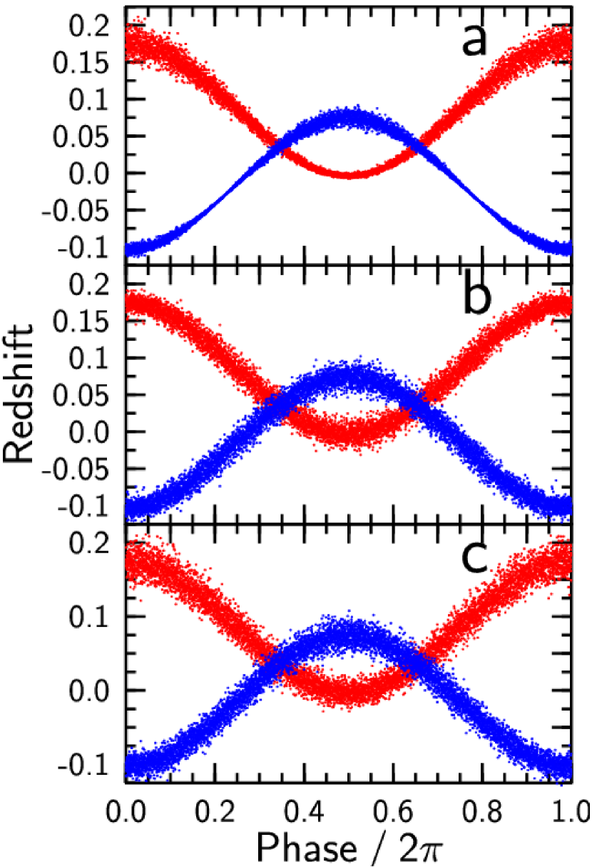
Figure 1: Demonstration that the dispersion in redshift with phase is unaffected by velocity variations as long as they are accompanied by pointing variations: (a) random variations in velocity drawn from a gaussian of half-width 0.013$c$, (b) random variations in $\theta$ and in phase drawn from gaussian distributions of 2.7 deg and 2.95 days respectively and (c) uncorrelated variations in all three of the quantities above.

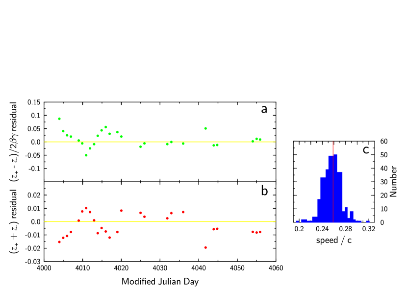
Figure 2: (a) and (b) examples of angular and speed residuals versus time. The variations suggest anti-correlation, § 3. (c) Distribution of speeds from the data compiled by Collins. The mean is indicated by the vertical red line, and the standard deviation in $\beta$ is 0.013.

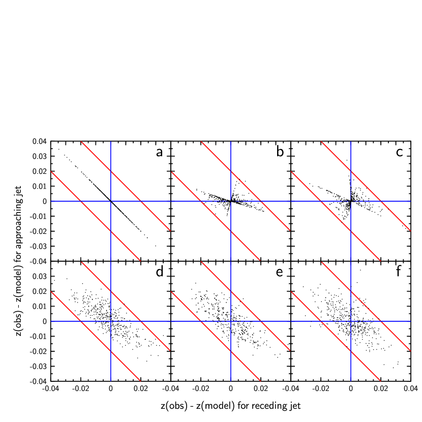
Figure 6: The effect on redshift residuals in each jet for deviations from the kinematic model in $\theta$, $\beta$ and $\phi$, for each date on which there is a redshift pair (replicating the sampling function). (a) Variations only in $\theta$, drawn from a gaussian distribution with half-width 2.7 degrees. The form of this plot, points lying only on the $y=-x$ line, is identical for variations only in $\phi$, or for variations in both $\phi$ and $\theta$. (b) Speed-only variations (on a given day $\beta$ is drawn from a gaussian of half-width 0.013 — Fig 2c). (c) Variations in $\beta$ anti-correlated with those in $\theta$: on a given synthesized observation date the same randomly-drawn number from a gaussian is scaled by 0.013 for the speed variation and by $-2.7$ degrees for the $\theta$ variation. (d) As (c), but with $\theta$ partially anti-correlated with $\beta$ and uncorrelated $\phi$ fluctuations (as Table 1). (e) As (d), but the duration of the $\beta$-variations, and that of the correlated $\theta$-component, is drawn from a gaussian of half-width 2 days. (f) Observed residuals.

References

- Blundell & Bowler (2004) Blundell, K. M., & Bowler, M. G. 2004, ApJ, 616, L159
- Charles et al (2004) Charles, P.A. et al, 2004, RevMexAA, 20, 50
- Crampton & Hutchings (1981) Crampton, D. & Hutchings, J.B. 1981, ApJ, 251, 604
- Collins & Scher (2002) Collins, G.W. & Scher, R.W., 2002, MNRAS, 336, 1011
- Collins & Scher (2000) Collins, G.W. & Scher, R.W., 2000, in “the Kth Reunion”, ed A.G.D. Philip, L. Davis Press, Schenectady, NY, pg105
- Eikenberry et al (2001) Eikenberry, S.S. et al, 2001, ApJ, 561, 1027
- Fabrika & Bychkova (1990) Fabrika, S. N. & Bychkova, L. V. 1990, A&A, 240, L5
- Gies et al (2002) Gies, D.R., Huang, W. & McSwain, M.V., 2002, ApJ, 578, l67
- Katz & Piran (1982) Katz, J. I. & Piran, T. 1982, Astrophys. Lett., 23, 11
- Katz et al (1982) Katz, J. I., Anderson, S. F., Grandi, S. A., & Margon, B. 1982, ApJ, 260, 780
- Margon (1984) Margon, B. 1984, ARA&A, 22, 507
- Newsom & Collins (1982) Newsom, G.H. & Collins, G.W., 1982, ApJ, 262, 714
- Roberts et al (1987) Roberts, D.H., Lehar, J. & Dreher, J.W., 1987, AJ, 93, 968