Generalised cosmological scaling solutions
Abstract
Motivated by the recent interest in cosmologies arising from energy density modifications to the Friedmann equation, we analyse the scaling behaviour for a broad class of these cosmologies comprised of scalar fields and background barotropic fluid sources. In particular, we determine the corresponding scalar field potentials which lead to attractor scaling solutions in a wide class of braneworld and dark energy scenarios. We show how a number of recent proposals for modifying the Friedmann equation can be thought of as being dual to one another, and determine the conditions under which such dualities arise.
pacs:
pacs: 98.80.CqI Introduction
The Friedmann equation is one of the cornerstones of modern cosmology relating the expansion of the Universe to the total energy density within it. It forms the starting point for almost all investigations in cosmology. However, over the past few years, possible corrections to the Friedmann equation have been derived or proposed in a number of different contexts, generally inspired by braneworld investigations. These corrections are often of a form that involves the total energy density , and are such that they tend to play a role early in the history of the Universe, fading away as we enter the late–time, post–nucleosynthesis era (although that is not always the case as we shall see). Up to now, the different models have been presented in the literature without any attempt to relate them. In this paper, by introducing a generalised form for the correction, we will provide a formalism which allows us to relate a large class of modified Friedmann cosmologies. Assuming the total energy density to be comprised of a canonical scalar field with potential , together with some form of barotropic fluid, we will demonstrate how the existence of scaling solutions determines the form of , and in doing so we will establish a direct relation between the form of the potential and the functional form of the modification to the Friedmann equation. Scaling (attractor) solutions in cosmology are very important because they allow one to understand the asymptotic behaviour of a particular cosmology and to determine whether such behaviour is stable or not. They have also been advocated by a number of authors as a way of establishing the behaviour of general scalar fields in a cosmological setting both in the context of conventional Friedmann cosmologies Ratra_Peebles ; Steinhardt ; trac ; CLW ; ferreira ; Liddle ; moduli_stabilization ; sahni ; delaMacorra:1999ff ; Ng:2001hs and in particular classes of modified Friedmann cosmologies Copeland:2000hn ; Huey:2001ae ; Sahni:2001qp ; Huey:2001ah ; Majumdar:2001mm ; Nunes:2002wz ; vandenhoogen ; Lidsey:2003sj ; Tsujikawa:2003zd ; Sami:2004ic ; Savchenko:2002mi ; Calcagni:2004bh ; Tsujikawa:2004dp .
In section II we present the equations of motion arising out of the modified Friedmann equations and introduce variables which allow the scaling solutions to be determined. The general conditions for scaling behaviour are then established in Section III and we show that these can be written as a closed form relationship between the scalar field and the functional form of the modification to the Friedmann equation. In section IV we demonstrate the existence of duality symmetries between different scaling solutions, and determine the conditions which must be satisfied in terms of the modification to the Friedmann equation for such duality properties to be obtained. Section V then applies the results of the previous sections to a general class of models, evaluating the scaling potentials (and their duals), as well as the explicit evolution of the scale factor in the scaling regimes. In particular, we apply the technique to a number of recently investigated cosmologies of relevance both to braneworld and dark energy scenarios, including the Randall–Sundrum R_S , Shtanov–Sahni Shtanov:2002mb and Cardassian Freese:2002sq models. The Dvali-Gabadadze-Porrati Dvali:2000hr braneworld scenario is investigated in Section VI and we summarize our results in section VII. Throughout units are chosen such that .
II Equations of motion
We consider spatially flat Friedmann–Robertson–Walker (FRW) cosmologies such that the dynamics is determined by an effective Friedmann equation of the form
| (1) |
where is the Hubble parameter, is the scale factor, is the total energy density of the universe, a dot denotes differentiation with respect to cosmic time and is the four–dimensional Planck mass. Modifications to standard relativistic cosmology are parametrized by the correction function and this is assumed to be positive–definite without loss of generality.
We will investigate models where the universe is sourced by a self–interacting scalar field with potential together with a barotropic fluid with equation of state , where is the adiabatic index. The energy density and pressure of the scalar field are given by and , respectively. As in conventional cosmologies, we assume that the energy–momenta of these matter fields is covariantly conserved and this implies that
| (2) | |||||
| (3) |
Eqs. (1)–(3) close the system that determines the cosmic dynamics.
In standard cosmology the stability of scaling solutions is analyzed by introducing the variables CLW :
| (4) |
and rewriting the field equations as an autonomous system. Following Huey:2001ae ; Huey:2001ah , we define the new pair of variables:
| (5) |
that are related to those of Eq. (4) by
| (6) |
where for expanding and contracting universes, respectively. In what follows, we consider expanding models unless otherwise stated.
When expressed in terms of the new variables (5), the equations of motion (1)–(3) can be written in the form:
| (9) | |||||
where
| (10) | |||||
| (11) |
and a prime denotes differentiation with respect to the logarithm of the scale factor, . As in Ref. Ng:2001hs , Eqs. (10) and (11) generalize the expressions introduced in Refs. CLW ; Huey:2001ah ; delaMacorra:1999ff ; Steinhardt . In particular, is related to the parameter introduced in Ref. CLW such that
| (12) |
We refer to as the ‘scaling parameter’.
The system of equations (II)–(11) for the variables , and do not appear to be closed due to the presence of the term involving in Eq. (9). However, it follows from Eqs. (5), (10) and (11) that we have , and and hence that . This implies that the equations are indeed closed.
The definition of the total energy density implies that the variables (5) satisfy the constraint equation
| (13) |
and, since the energy density of the barotropic fluid is semi–positive–definite, any cosmological model can be represented as a trajectory in the –plane that is bounded within the unit circle, i.e., . Furthermore, since by definition, it is sufficient to consider the evolution in the upper half of the disc.
Eqs. (II-9) exhibit an important property. For the case where is constant, they have an identical form to that of the plane–autonomous system of standard relativistic cosmology that is formulated in terms of the variables . This duality immediately implies that the system (II-II) admits an identical set of critical points to that of the standard scenario when these solutions are expressed in terms of the variables .
A further consequence of such a duality is that the stability of each fixed point solution can be determined directly from the stability analysis of Ref. CLW . In total, there are five critical solutions to Eqs. (II) and (II) where the variables are constants. Three of these represent the unstable solutions ,, for all values of and . The value of determines the nature of the other two points. For , there exists an attractor solution
| (14) |
where the effective adiabatic index of the scalar field, defined by
| (15) |
satisfies the condition . For this late–time attractor solution, the relative contribution of the scalar field’s energy density to the total energy density of the universe is constant, , and consequently, the energy densities of the scalar field and fluid redshift at the same rate as the universe expands.
The fifth critical point arises if and is given by
| (16) |
This corresponds to the case where the scalar field dominates the fluid and has an effective adiabatic index . The solution is stable if , i.e., .
III General Conditions for Scaling Solutions
Since the expressions (6) and (12) relating the standard and modified FRW cosmologies involve the correction function , the scalar field potential that gives rise to the fixed point attractor solutions (II) and (II) in a given generalized scenario will depend on the specific form of this function. In particular, the potential will differ from the purely exponential form that leads to scaling solutions in the conventional FRW model. In this section we establish the correspondence between the modified Friedmann equation and the scaling potential.
It can be shown by direct substitution that both sets of critical points (II) and (II) represent solutions to the field equations (II)–(9) of the form if the relation
| (17) |
is satisfied. Since for these solutions, Eq. (17) may be written in the form
| (18) |
and multiplying Eq. (18) by then implies that
| (19) |
Eq. (19) may be integrated twice to yield a necessary and sufficient condition on the scalar field potential if the solution is to represent a scaling solution for a given choice of correction function . We find the important result:
| (20) |
where one of the integration constants has been set to zero without loss of generality by performing a linear shift in the value of the scalar field and the constant of proportionality on the right–hand side follows by requiring consistency with Eq. (10).
It is also of interest to determine the evolution of the scale factor for a given class of scaling solutions. Since is a non–zero constant for these solutions, Eq. (5) implies that the scalar field is a monotonically varying function of proper time . It is natural, therefore, to view the value of the field as the dynamical variable of the system and to express all time–dependent parameters in terms of this variable.
In general, the scalar field Eq. (3) can be expressed in the form
| (21) |
or, equivalently, as
| (22) |
It then follows from the definition of the Hubble parameter that
| (23) |
and substituting Eq. (23) into Eq. (1) implies that the Friedmann equation can be expressed in the form
| (24) |
Introducing a new variable
| (25) |
simplifies Eq. (24) to
| (26) |
and the scale factor is then determined up to a single quadrature:
| (27) |
Thus, for a given cosmological scenario characterized by a correction function , the potential (and equivalently the total energy density) yielding the scaling solution is determined by integrating Eq. (20). Integration of Eq. (25) then yields the dependence of on the scalar field and the evolution of the scale factor follows after integration of Eq. (27). Finally, the time–dependence of the scale factor can in principle be deduced by integrating Eq. (22),
| (28) |
and inverting the result.
In the following section, we employ the above formalism to establish a link between different classes of scaling solutions that arise for various choices of the modification to the Friedmann equation.
IV Duality between Scaling Solutions
A duality between different scaling solutions can be established by noting that Eq. (26) is invariant under the simultaneous interchange
| (29) |
where is an arbitrary constant. This symmetry implies that a given scaling solution may be employed as a seed to generate a new scaling cosmology for a different Friedmann equation and associated scalar field potential. To be specific, let us consider the scaling solution parametrized by the functions that arises for a specific choice of correction function . We now denote the ‘dual’ scaling solution as and assume an ansatz of the form
| (30) |
The new scale factor is then determined from Eq. (27):
| (31) |
However, since the function is itself a solution to the Friedmann equation (26), Eq. (31) simplifies after integration to
| (32) |
modulo an arbitrary (constant) prefactor.
We may now determine the condition that the dual correction function must satisfy for the solution (32) to also represent a scaling solution that satisfies Eq. (20). If we assume a priori that the two solutions represent scaling solutions characterized by , respectively, Eq. (20) implies that
| (33) |
It then follows, after substitution of Eq. (24) into the right–hand side of Eq. (33), that
| (34) |
and Eq. (26) then implies that
| (35) |
On the other hand, substituting the ansatz (30) into Eq. (35) and employing Eq. (24) for the positive–branch solution yields the condition
| (36) |
Consistency with Eq. (20) therefore implies that a necessary and sufficient condition for the dual cosmology to represent a scaling solution is that the correction functions arising in the respective Friedmann equations must be proportional to the inverse of each other when both are expressed as functions of the scalar field:
| (37) |
It is interesting that the standard relativistic cosmology represents the self–dual model when .
Finally, we find after substituting Eq. (37) into Eq. (33) and employing Eq. (25) that the energy density of the dual scaling solution is given by
| (38) |
The dual potential then follows immediately from Eqs. (5) and (25):
| (39) |
In the following section we employ the techniques developed above to determine scaling solutions (and their duals) in a number of different cosmological settings.
V Unification of modified Friedmann cosmologies
V.1 A Generalized Class of Scaling Cosmologies
A wide class of scenarios that have been considered recently predict deviations from the standard cosmology of the form
| (40) |
where is an arbitrary dimensionless constant and is an arbitrary constant with dimension . In this case, the form of the potential leading to scaling (fixed point) solutions is determined by integrating Eq. (20). It is found that
| (41) |
if and
| (42) |
if .
Given the form of the scalar potential (41), the parametric solution for the case is determined by integrating Eqs. (25) and (27), respectively:
| (43) |
The time dependence of the solution follows by substituting Eq. (43) into Eq. (40) to yield the Friedmann correction function:
| (44) |
and then evaluating the integrand in Eq. (28):
| (45) |
The integral (45) can be performed analytically for various choices of , whereas the late–time behaviour can be analysed for arbitrary . In particular, we find from Eq. (45) that the late–time limit corresponds to large , and it therefore follows from Eq. (44) that as . This in turn is the limit corresponding to the case of an exponential potential.
The corresponding scaling solution for driven by the potential (42) is deduced by applying the duality transformation (29) to the solution (43) for a particular value of the constant , where the scaling parameters are chosen to be equal, . For the case where , the duality transformation (37) implies that the dual correction function is given by
| (46) |
whilst integrating Eq. (39) with the form for given in Eq. (43) implies that the dual potential has precisely the form of Eq. (42). We may conclude, therefore, that the dual correction function is given by Eq. (40) with . In this sense, a model with and a specific value of is twinned with the model where the value of is the same but the sign of is changed. In general, the dual scale factor is deduced from Eqs. (32) and (43):
| (47) |
and the time–dependence follows from Eq. (28):
| (48) |
It is of course trivial to show that for this choice of , the standard cosmology solution corresponding to the case reproduces the well known exponential potential for the scalar field Lucchin .
In the following subsections, we consider some of the specific models that belong to the class of corrections given by Eq. (40).
V.2 Randall-Sundrum Type II braneworld cosmology
The case and corresponds to the Randall–Sundrum type II (R-S II) braneworld scenario R_S ; cline ; SMS ; Binetruy , where a co–dimension one brane with positive tension is embedded in five–dimensional Anti–de Sitter () space:
| (49) |
For this case, the scaling potential yielding the fixed point solution is given by
| (50) |
and the time–dependences of the scalar field and scale factor are deduced by evaluating the integral (45) for and substituting the result into Eq. (43):
| (51) | |||
| (52) |
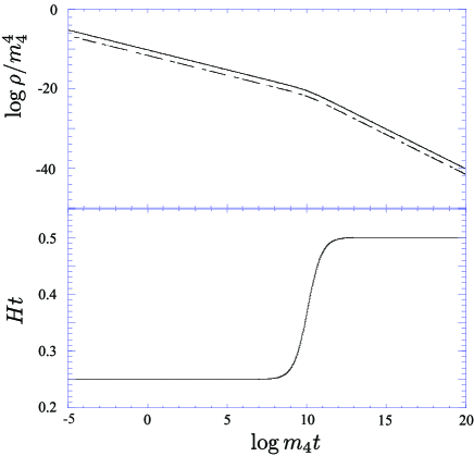
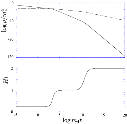
These results for the scaling solutions associated with the R-S II model confirm those previously obtained using a different method in Ref. Hawkins:2000dq . An important feature of our approach is that it shows the solution is a fixed point attractor solution. Another important feature that emerges is that in the limit where the quadratic energy density term dominates, i.e., when , the potential (50) asymptotes to , consistent with earlier analyses MMY ; Maeda:2000mf . Similarly, once the energy density has decreased so that , the value of the scalar field becomes large, and , in agreement with general relativistic results trac ; CLW .
In Figs. 1-2, we confirm numerically how the above potential leads to the expected attractor solutions for a model with a barotropic fluid of radiation ().
V.3 Shtanov-Sahni braneworld cosmology
The case and represents a class of braneworld inspired cosmologies due to Shtanov and Sahni (S-S) Shtanov:2001pk ; Kofinas:2001es ; Shtanov:2002mb . In this scenario, a co–dimension one brane with negative tension is embedded in a five–dimensional conformally flat Einstein space, where the signature of the fifth dimension is timelike. In this model, the deviation from the conventional Friedmann cosmology is characterised by
| (53) |
This model has recently been invoked to develop a non–singular oscillating universe, where the turning points in both the contracting and expanding phases are induced by the quadratic correction Brown:2004cs .
The S-S braneworld is dual to that of the RS-II scenario in the sense discussed above. The scaling potential follows directly from Eq. (42):
| (54) |
whereas the time–dependences of the scalar field and scale factor follow from Eqs. (48) and (47), respectively, after substituting for and :
| (55) | |||
| (56) |
Such a scaling solution is phenomenologically interesting since it represents a non–singular bouncing cosmology. The universe collapses from infinity to a finite size at and then bounces into an expanding phase. The scalar field rolls up the potential during the collapse, reaches the maximum of the potential at at the instant of the bounce, and then rolls monotonically down the other side during the expansion era.
V.4 Cardassian cosmology
In the above classes of models, the modifications to the Friedmann equation become significant at high energy scales (early times). On the other hand, recent CMB and large–scale structure observations indicate that the universe is entering a stage of accelerated expansion at the present epoch and a number of phenomenological models have been developed in an attempt to provide a geometrical interpretation of these observations. In Cardassian cosmology Freese:2002sq ; Freese:2002gv , for example, the modification term in the Friedmann equation is given by Eq. (40) with and Freese:2002sq ; Freese:2002gv :
| (57) |
and the present–day cosmological acceleration can be explained even when the energy density is comprised of only ordinary matter sources if . The characteristic feature of this model, therefore, is that the modification term becomes significant at late times.
Although no scalar field is present in the scenario considered in Refs. Freese:2002sq ; Freese:2002gv , it is instructive to show that the equivalent background cosmology can be obtained from a model comprised of a barotropic fluid and a self–interacting scalar field. We see immediately from Eq. (41) that the corresponding potential which provides the fixed point attractor solution is given by
| (58) |
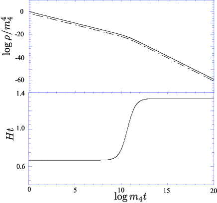
and in Fig. 3 we demonstrate numerically how the above potential leads to the expected attractor solution. Although such a homogeneous solution is indistinguishable from the purely perfect fluid background, it is possible that the presence of a scalar field may modify the evolution of perturbations and the clustering properties of matter. In principle, this could result in potentially observational signatures Bartolo:2003ad and a scaling solution of this type provides a framework for quantitatively investigating the evolution of perturbations in these models.
Finally, before concluding this Section, we illustrate the duality transformation that relates the Cardassian cosmologies with the S-S braneworld. Denoting the former with a subscript ‘’ and the latter by ‘’, we may substitute the form for in the Cardassian scenario, as given by Eq. (43), into Eq. (38) to deduce that
| (59) |
This reduces to the S-S scaling potential Eq. (42) (with and ) when and . Moreover, in this case, it can be verified that the dual correction function satisfying Eq. (37) reduces to Eq. (46) with and .
We now proceed in following section to determine the scaling solutions in a further braneworld scenario, where the corrections to the Friedmann equation become significant at late times.
VI Dvali-Gabadadze-Porrati braneworld cosmology
The Dvali–Gabadadze–Porrati (DGP) braneworld scenario Dvali:2000hr ; Deffayet:2000uy corresponds to a 3–brane embedded in flat five–dimensional Minkowski spacetime, where a Ricci scalar term is included in the brane action. All energy–momentum is confined to the brane since the bulk is empty. The modified Friedmann equation for the DGP model is given by Deffayet:2000uy
| (60) |
where and is the five–dimensional Planck scale. In the DGP model, gravity behaves as four–dimensional Einstein gravity at short scales, whereas it propagates into the bulk at large scales. This induces corrections to the standard Friedmann equation at low energies and the parameter determines the scale at which these corrections become important. There are two inequivalent ways of embedding the brane in the bulk and this is reflected in the different choices of sign in Eq. (60). In this section, we refer to these as the and branches, respectively. In subsequent expressions, where different signs may be taken, the upper case corresponds to the branch.
It proves convenient to express the Friedmann equation (60) in the equivalent form
| (61) |
where
| (62) |
For the branch, the late–time attractor is de Sitter (exponential) expansion for any decreasing energy density Deffayet:2000uy . For the branch, on the other hand, expanding Eq. (61) as a Taylor series to lowest–order implies that . Modulo a rescaling of the four–dimensional Planck mass, this corresponds formally to the high–energy limit of the R-S II braneworld (49). Consequently, the early–time analysis of the latter model performed in Ref. Mizuno:2004xj is directly applicable to the late–time behaviour of this branch of the DGP model. In particular, we may conclude immediately that the potential driving the scaling solution in this limit is the inverse power–law potential .
A direct comparison between Eqs. (1) and (61) implies that the Friedmann correction function is given by
| (63) |
In order to derive the scaling solutions, we define a new variable, :
| (64) |
Substituting Eq. (63) into Eq. (20) then implies that the solution represents a scaling solution if
| (65) |
and the integral (65) may be evaluated to yield the form of the potential:
| (66) |
The corresponding time dependence of the scaling solution can also be determined. In terms of the variable (64), the Friedmann equation (61) simplifies to
| (67) |
for the branch, and
| (68) |
for the branch. Recalling that and for the scaling solution, it follows that the scalar field equation (21) transforms to
| (69) |
after substitution of Eq. (64). Substituting Eqs. (67) and (68) for the and branches, respectively, and evaluating the integral (69) then implies that
| (70) |
VII Summary
In this paper we have brought together a number of recent approaches to cosmology which involve modifications of the Friedmann equation. By introducing the general function as the way of parametrising the modification, we have been able to establish the conditions under which the new system enters scaling solutions. Considering the case where the energy density is comprised of a scalar field and background barotropic fluid, we have obtained the general relationship that would have to be satisfied between the evolving scalar field and . In particular, we have obtained the corresponding potential which leads to scaling solutions and, for a rather general class of functions of , we have shown that there exist dual solutions which also exhibit similar scaling behaviour. This has allowed us to relate solutions which would otherwise appear quite distinct, including those involving collapsing and expanding cosmologies.
Moreover, the duality can directly relate singular and non–singular cosmologies. To illustrate this property, consider a particular scaling solution that is singular in the sense that the scale factor vanishes at . (The value of the scalar field can be chosen to be without loss of generality). Suppose, however, that the logarithmic derivative of the scale factor with respect to the field is non–zero at this point, , and furthermore, that the scale factor is a monotonic function with a finite first derivative for all physical (non–zero) values of the field. These properties are satisfied, for example, in the R-S II and Cardassian models.
The qualitative behaviour of the dual solution, , is then determined from Eq. (31). If we define a new parameter , the value of the scale factor is simply given by the area under the curve , where the field evolves from zero to some value . (We are assuming implicitly that and again without loss of generality). However, due to the exponential nature of Eq. (31) the initial value of the dual scale factor is non–zero and this results in a non–singular background.
On the other hand, the time reversal of the seed solution would result in a collapsing dual model where the limits in the integral (31) are taken from to zero. Consequently, the dual solution can be analytically continued through into a contracting phase. In this sense, therefore, any singular (expanding) scaling solution satisfying the above (very weak) conditions can generate a non–singular bouncing cosmology, where the latter is associated with a combination of the seed solution and its time reversal. For fixed values of , the collapsing phase of the bouncing solution will be unstable if the expanding phase is stable, and vice–versa. In principle, however, different seed solutions may be employed to generate distinct and stable collapsing and expanding branches that can be smoothly joined at the bounce.
This opens up the possibility that such dualities will allow us to relate singular cosmologies to non-singular bouncing cosmologies, a topic presently of considerable interest in cosmology.
Finally, we have argued that the type of correction given by Eq. (40) arises in a number of particle physics motivated models. Further examples arise in the limit where . In particular, the case corresponds to the high–energy limit of the Gauss–Bonnet braneworld gb . In this model, the R-S II scenario is generalized to include a Gauss–Bonnet combination of curvature invariants in the five–dimensional bulk action. More generally, effective Friedmann equations of the form , where is arbitrary chung , can arise in models based on Hořava–Witten theory compactified on a Calabi–Yau three–fold H_W . Generalized scaling solutions driven by corrections of this form were recently investigated for a variety of scalar field models Tsujikawa:2004dp .
Future directions involving the use of the duality properties of these models would include an extension of our analysis to negative potentials, thereby allowing us to link these classes of solutions with those arising in the cyclic/ekpyrotic scenario Steinhardt:2001st . On the other hand, as we have seen, the more general corrections proposed in Dvali:2000hr ; Deffayet:2000uy that arise due to modifications of gravity on large scales can lead to an explanation of the present cosmic acceleration without introducing dark energy Lue:2004za . It would be interesting to investigate the impact that the duality transformations we have described have on such a scenario.
Acknowledgments
EJC would like to thank the Aspen Center for Physics for their hospitality during the time part of this paper was completed. SM would like to thank Kei-ichi Maeda for continuous encouragement and is grateful to the University of Sussex for their hospitality during a period when this work was initiated.
References
- (1) B. Ratra and P. J. E. Peebles, Phys. Rev. D 37, 3406 (1988).
- (2) R. R. Caldwell, R. Dave and P. J. Steinhardt, Phys. Rev. Lett. 80, 1582 (1998) [arXiv:astro-ph/9708069]; I. Zlatev, L. M. Wang and P. J. Steinhardt, Phys. Rev. Lett. 82, 896 (1999) [arXiv:astro-ph/9807002]; P. J. Steinhardt, L. M. Wang and I. Zlatev, Phys. Rev. D 59, 123504 (1999) [arXiv:astro-ph/9812313].
- (3) C. Wetterich, Nucl. Phys. B302, 668 (1988).
- (4) E. J. Copeland, A. R. Liddle and D. Wands, Phys. Rev. D 57, 4686 (1998) [arXiv:gr-qc/9711068].
- (5) P. G. Ferreira and M. Joyce, Phys. Rev. D 58, 023503 (1998) [arXiv:astro-ph/9711102].
- (6) A. R. Liddle and R. J. Scherrer, Phys. Rev. D 59, 023509 (1999) [arXiv:astro-ph/9809272].
- (7) T. Barreiro, B. de Carlos and E. J. Copeland, Phys. Rev. D 58, 083513 (1998) [arXiv:hep-th/9805005]; G. Huey, P. J. Steinhardt, B. A. Ovrut and D. Waldram, Phys. Lett. B 476, 379 (2000) [arXiv:hep-th/0001112]; T. Barreiro, B. de Carlos and N. J. Nunes, Phys. Lett. B 497, 136 (2001) [arXiv:hep-ph/0010102].
- (8) V. Sahni and A. Starobinsky, Int. J. Mod. Phys. D 9, 373 (2000) [arXiv:astro-ph/9904398].
- (9) A. de la Macorra and G. Piccinelli, Phys. Rev. D 61, 123503 (2000) [arXiv:hep-ph/9909459].
- (10) S. C. C. Ng, N. J. Nunes and F. Rosati, Phys. Rev. D 64, 083510 (2001) [arXiv:astro-ph/0107321].
- (11) E. J. Copeland, A. R. Liddle and J. E. Lidsey, Phys. Rev. D 64, 023509 (2001) [arXiv:astro-ph/0006421].
- (12) G. Huey and J. E. Lidsey, Phys. Lett. B 514, 217 (2001) [arXiv:astro-ph/0104006].
- (13) V. Sahni, M. Sami and T. Souradeep, Phys. Rev. D 65, 023518 (2002) [arXiv:gr-qc/0105121]; M. Sami and V. Sahni, arXiv:hep-th/0402086.
- (14) G. Huey and R. K. Tavakol, Phys. Rev. D 65, 043504 (2002) [arXiv:astro-ph/0108517].
- (15) A. S. Majumdar, Phys. Rev. D 64, 083503 (2001) [arXiv:astro-ph/0105518].
- (16) N. J. Nunes and E. J. Copeland, Phys. Rev. D 66, 043524 (2002) [arXiv:astro-ph/0204115].
- (17) R. J. van den Hoogen, A. A. Coley and Y. He, Phys. Rev. D 68, 023502 (2003) [arXiv:gr-qc/0212094]; R. J. van den Hoogen and J. Ibanez, Phys. Rev. D 67, 083510 (2003) [arXiv:gr-qc/0212095].
- (18) J. E. Lidsey and N. J. Nunes, Phys. Rev. D 67, 103510 (2003) [arXiv:astro-ph/0303168].
- (19) S. Tsujikawa and A. R. Liddle, JCAP 0403, 001 (2004) [arXiv:astro-ph/0312162].
- (20) M. Sami and N. Dadhich, arXiv:hep-th/0405016.
- (21) N. Y. Savchenko and A. V. Toporensky, Class. Quant. Grav. 20, 2553 (2003) [arXiv:gr-qc/0212104].
- (22) G. Calcagni, Phys. Rev. D 69, 103508 (2004) [arXiv:hep-ph/0402126].
- (23) M. Sami, N. Savchenko and A. Toporensky, arXiv:hep-th/0408140; S. Tsujikawa and M. Sami, arXiv:hep-th/0409212.
- (24) L. Randall and R. Sundrum, Phys. Rev. Lett. 83, 3370 (1999) [arXiv:hep-ph/9905221]; L. Randall and R. Sundrum, Phys. Rev. Lett. 83, 4690 (1999) [arXiv:hep-th/9906064].
- (25) Y. Shtanov and V. Sahni, Phys. Lett. B 557, 1 (2003) [arXiv:gr-qc/0208047].
- (26) K. Freese and M. Lewis, Phys. Lett. B 540, 1 (2002) [arXiv:astro-ph/0201229].
- (27) G. R. Dvali, G. Gabadadze and M. Porrati, Phys. Lett. B 485, 208 (2000) [arXiv:hep-th/0005016].
- (28) F. Lucchin and S. Matarrese, Phys. Rev. D 32, 1316 (1985).
- (29) S. Mizuno, K. Maeda and K. Yamamoto, Phys. Rev. D 67, 023516 (2003) [arXiv:hep-ph/0205292].
- (30) K. Maeda, Phys. Rev. D 64, 123525 (2001) [arXiv:astro-ph/0012313]; S. Mizuno and K. Maeda, Phys. Rev. D 64, 123521 (2001) [arXiv:hep-ph/0108012].
- (31) S. Mizuno, S. J. Lee and E. J. Copeland, arXiv:astro-ph/0405490.
- (32) R. M. Hawkins and J. E. Lidsey, Phys. Rev. D 63, 041301 (2001) [arXiv:gr-qc/0011060].
- (33) V. A. Rubakov and M. E. Shaposhnikov, Phys. Lett. 125B, 139 (1983); K. Akama, Lect. Notes Phys. 176, 267 (1982) [arXiv:hep-th/0001113].
- (34) P. Hořava and E. Witten, Nucl. Phys. B460, 506 (1996) [arXiv:hep-th/9510209]; P. Hořava and E. Witten, Nucl. Phys. B475, 94 (1996) [arXiv:hep-th/9603142].
- (35) N. Arkani-Hamed, S. Dimopoulos and G. R. Dvali, Phys. Lett. B 429, 263 (1998) [arXiv:hep-ph/9803315]; I. Antoniadis, N. Arkani-Hamed, S. Dimopoulos and G. R. Dvali, Phys. Lett. B 436, 257 (1998) [arXiv:hep-ph/9804398].
- (36) C. Csaki, M. Graesser, C. F. Kolda, and J. Terning, Phys. Lett. B 462, 34 (1999) [arXiv:hep-ph/9906513]; J. M. Cline, C. Grojean and G. Servant, Phys. Rev. Lett. 83, 4245 (1999) [arXiv:9906523].
- (37) T. Shiromizu, K. Maeda and M. Sasaki, Phys. Rev. D 62, 024012 (2000) [arXiv:gr-qc/9910076].
- (38) P. Binetruy, C. Deffayet and D. Langlois, Nucl. Phys. B 565, 269 (2000) [arXiv:hep-th/9905012]; P. Binetruy, C. Deffayet, U. Ellwanger and D. Langlois, Phys. Lett. B 477, 285 (2000) [arXiv:hep-th/9910219].
- (39) Y. V. Shtanov, Phys. Lett. B 541, 177 (2002) [arXiv:hep-ph/0108153].
- (40) G. Kofinas, JHEP 0108, 034 (2001) [arXiv:hep-th/0108013].
- (41) D. J. H. Chung and K. Freese, Phys. Rev. D 61, 023511 (2000) [hep-ph/9906542].
- (42) M. G. Brown, K. Freese and W. H. Kinney, arXiv:astro-ph/0405353.
- (43) K. Freese, Nucl. Phys. Proc. Suppl. 124, 50 (2003) [arXiv:hep-ph/0208264].
- (44) N. Bartolo, P. S. Corasaniti, A. R. Liddle and M. Malquarti, Phys. Rev. D 70, 043532 (2004) [arXiv:astro-ph/0311503].
- (45) C. Deffayet, Phys. Lett. B 502, 199 (2001) [arXiv:hep-th/0010186].
- (46) P. J. Steinhardt and N. Turok, Phys. Rev. D 65, 126003 (2002) [arXiv:hep-th/0111098].
- (47) A. Lue and G. D. Starkman, arXiv:astro-ph/0408246.
- (48) C. Charmousis and J. Dufaux, Class. Quantum Grav. 19, 4671 (2002) [arXiv:hep-th/0202107]; S. C. Davis, Phys. Rev. D 67, 024030 (2003) [arXiv:hep-th/0208205]; E. Gravanis and S. Willison, Phys. Lett. B 562, 118 (2003), [arXiv:hep-th/0209076]; J. E. Lidsey and N. Nunes, Phys. Rev. D 67, 103510 (2003) [arXiv:astro-ph/0303168].