Testing the Universality of the $(U-V)$ Color-Magnitude Relations for Nearby Clusters of Galaxies

Abstract

We present a detailed $(U-V)$ color-magnitude relation (CMR) analysis for three local ($z<0.06$) clusters of galaxies. From square-degree imaging of the Abell clusters A85, A496, and A754, we select 637 galaxies down to $L\sim 0.1L^{\star}_{V}$ with spectroscopic membership, which minimizes uncertain field contamination corrections. To characterize the degree of CMR uniformity among nearby clusters, we use a maximum likelihood technique to quantify the CMR properties of the red galaxies in each cluster. We find that these clusters have similar CMRs with a mean color of $(U-V)=1.40$ at $M_{V}=-20+5\log_{10}h$, and narrow limits of intrinsic color scatter [0.047,0.079] and slope [-0.094,-0.075]. If we restrict our analysis to the core cluster population of red galaxies, the resultant CMRs are in close agreement with that of the Coma Cluster, the only local cluster with a rest-frame $(U-V)$ CMR determination of comparable precision. Therefore, the CMR uniformity of present-day clusters spans a fairly wide range of cluster masses. We test how sensitive the CMR uniformity is to variations in color aperture size and sample selection, and we find at most slightly wider limits of scatter [0.047,0.112] and slope [-0.104,-0.054]. This upper limit for $(U-V)$ scatter is consistent with the bulk of the stellar populations of red cluster galaxies forming before $z=1.2$, with a maximum age spread of 5.2 Gyr. In addition, we note that using colors from apertures containing equal fractions of galactic light does not remove the CMR slope and that none of the slopes exhibit a break as claimed by Metcalf et al. Our findings expand the single Coma data point and provide a much-needed $z=0$ baseline for comparisons to high redshift cluster CMRs at the same rest-frame wavelengths. The range in CMR scatter that we find among nearby clusters is consistent with the values reported for clusters at higher redshifts, further suggesting that there has been little evolution in the stellar populations of red-sequence cluster galaxies out to at least $z\sim 1$. To identify the most recently accreted cluster galaxies, we divide each cluster’s membership into three galaxy populations based on $(U-V)$ color relative to the well-defined CMR. Blue and moderately blue galaxies make up $18-23\%$ by number of each cluster population more luminous than $0.1L^{\star}$. Our color-magnitude division should represent a rough time since cluster accretion. In testing this hypothesis, we find that blue galaxies are spatially, kinematically, and morphologically distinct from red cluster galaxies. Even in projection, the blue galaxies reside towards the outskirts of the cluster and appear to avoid the inner half megaparsec, in contrast with the increasing density of red sequence galaxies towards the cluster center. In addition, the blue galaxies have velocity distributions relative to the cluster rest frame that are flatter, and some have different means, compared to the roughly Gaussian distribution of red member velocities. Members with the bluest colors tend to be disk-like or irregular in appearance compared to the red galaxies, which have mostly early-type (E/S0) morphologies. Moderately blue cluster galaxies may be an intermediate mix with a fraction of small bulge-to-disk ratio S0s, yet these require closer scrutiny. The spatial, kinematic, and morphological distinctions between blue and red cluster galaxies provide further evidence that CMR-relative color is related to time since cluster infall, and that bluer members are indeed the most recently accreted field spirals as expected in an hierarchical universe.

1 Introduction

The color-magnitude (C-M) diagrams of rich galaxy clusters provide information essential to understanding the formation and evolution of cluster members. For example, the early-type (E/S0) galaxies in clusters follow a well-defined correlation of increasingly red galaxy color with growing luminosity (e.g. Visvanathan & Sandage, 1977; Bower, Lucey, & Ellis, 1992b; Hogg et al., 2004), which is often labeled the color-magnitude relation (CMR) or the “red sequence”. The apparent uniformity of the slope and the small color scatter of the CMR are interpreted conventionally as evidence that these galaxies have ancient stellar populations ($z_{\rm f}\sim 2-3$) with a small range in relative ages (Bower, Lucey, & Ellis, 1992b; Lubin, 1996; Kodama et al., 1998; Bower, Kodama, & Terlevich, 1998). Furthermore, if the CMR is well-determined, it is possible to identify the population of most recently accreted cluster members by their blue colors relative to the CMR (Balogh, Navarro, & Morris, 2000; Kodama & Bower, 2001; Bicker et al., 2002). Such recent arrivals to the cluster environment make ideal tests of the picture of hierarchical cluster formation and the mechanisms that may affect the evolution of cluster galaxies.

Because of its particular sensitivity to recent star formation (SF), the near-UV C-M diagram (i.e., $U-V$ color vs. $V$-band absolute magnitude) has the potential to place the best constraints on the formation epoch and relative ages of the red sequence galaxies, as well as on the properties of the infalling population of cluster galaxies. Unfortunately, due to the difficulty in obtaining wide-field imaging and spectroscopic follow-up for large samples of cluster members, little is known about the near-UV properties of nearby cluster galaxies. In this paper, we present the results from a new wide-field spectroscopic and near-UV imaging study of galaxy clusters in the nearby ($z<0.06$) universe.

Constraining the era over which the stars in the oldest cluster galaxies formed is a subject of much study and debate (Bower, Kodama, & Terlevich, 1998; Gladders et al., 1998; Rose et al., 2001; Kodama & Bower, 2001; van Dokkum & Franx, 2001, and references therein). The near-UV CMRs of nearby clusters have an important role to play in addressing this question. Because $(U-V)$ color straddles the 4000 Å break, near-UV CMRs are more sensitive than red CMRs to any small differences in the star-formation histories (SFHs) of cluster galaxies. For example, simple stellar burst models (e.g. Worthey, 1994; Vazdekis et al., 1996) show that a stellar population with solar metallicity that formed $>10$ Gyr ago over a period of 4 Gyr has an intrinsic color scatter in $(U-V)$ that is roughly twice as large as in $(B-R)$, regardless of the model details (i.e. initial mass function, metallicity, etc.). If the near-UV CMRs of nearby clusters are uniform in slope and narrow in scatter, then the formation time and age spread for the stars can be better constrained than with $(B-R)$. Another constraint on this formation epoch can be obtained by comparing the near-UV CMRs of nearby clusters to the CMRs of distant clusters based on observations at red optical passbands, which correspond to the same rest-frame near-UV band. Recent work on distant clusters has shown that the CMR scatter based on rest-frame $(U-V)$ colors is quite small and homogeneous for redshifts $z>0.5$ (Ellis et al., 1997; Stanford, Eisenhardt, & Dickinson, 1998). The observed absence of evolution in the scatter of the near-UV CMR at moderate redshifts suggests an early formation time for the constituent stars, but a direct comparison to large, well-defined samples of $z\sim 0$ cluster galaxies is lacking.

Early work on the near-UV CMRs, which included only the brightest, early-type members of a few poorly-sampled nearby clusters, suggested that the near-UV CMRs are universal (Visvanathan & Sandage, 1977; Sandage & Visvanathan, 1978; Bower, Lucey, & Ellis, 1992b). More recent work has raised questions about the form of cluster CMRs. For example, there is controversy as to whether the slope of the relation changes at lower luminosities (Metcalfe, Godwin, & Peach, 1994). To date, Coma (A1656, $z=0.022$) remains the only rich cluster at low redshift with a well-defined near-UV CMR based on hundreds of spectroscopically-confirmed cluster members sampled from large cluster-centric distances ($>1$ Mpc; Terlevich, Caldwell, & Bower, 2001). As a consequence, it is hard to assess the degree of uniformity among cluster CMRs and to compare them with high redshift systems. Determining the near-UV CMRs for a larger sample of clusters as we have now done is therefore essential to resolve these issues.

Identifying the population of galaxies most recently accreted by the cluster is critical to (1) test how lower mass systems like galaxies and groups combine to form clusters and (2) determine the importance of factors that may influence the evolution of cluster galaxies, e.g. ram pressure stripping (Abadi, Moore, & Bower, 1999; Quilis, Moore, & Bower, 2000), gas consumption through starbursts (Hashimoto et al., 1998; Bekki, 1998; Fujita & Nagashima, 1999; Rose et al., 2001) or strangulation (Larson, Tinsley, & Caldwell, 1980; Balogh & Morris, 2000; Bekki, Couch, & Shioya, 2002), galaxy harassment (Moore, Lake, & Katz, 1998; Moore et al., 1999), and galaxy-galaxy interactions or mergers in infalling groups (Zabludoff et al., 1996; Zabludoff & Mulchaey, 1998). Compared to the population of old, early types that define the CMR, spectroscopic studies of galaxies with bluer colors at each luminosity show them to have younger luminosity-weighted mean ages (e.g. van Dokkum et al., 1998; Terlevich et al., 1999). Therefore, it follows that the bluest cluster members relative to the CMR have SF properties most similar to the field population of spirals, and thereby are likely to be the most recent cluster arrivals (Balogh, Navarro, & Morris, 2000; Kodama & Bower, 2001; Bicker et al., 2002). This population has only been identified in clusters at intermediate redshifts ($z>0.3$ Dressler et al., 1997; van Dokkum et al., 1998, 1999; Poggianti et al., 1999; Kodama et al., 2001). In nearby clusters, many of the infalling galaxies may lie at large projected radii $R_{\rm p}$ from the cluster center (Diaferio et al., 2001), making them difficult to observe with small area detectors. For example, nearby clusters appear to have small ($<5\%$) fractions of blue galaxies (Butcher & Oemler, 1978a, 1984), which is likely the result of an observational bias if new members are expected at large $R_{\rm p}$. Until quite recently only the cores ($R_{\rm p}<0.5$ $h^{-1}$ Mpc) of local ($z<0.1$) clusters had been imaged due to the limiting size of detectors and the large area these objects span on the sky. A detailed search for the most recent cluster arrivals in Abell clusters at $z<0.06$ requires wide-field imaging ($\geq 0.5$ degree per 1 $h^{-1}$ Mpc). Here we utilize a wide-field (one square degree) imaging campaign to acquire data for a large number of cluster galaxies out to $R_{\rm p}>1$ $h^{-1}$ Mpc . With our wide-field spectroscopic sample of nearby clusters, it is possible to ask whether the spatial, kinematic, and morphological properties of the bluest cluster galaxies support the picture that they are new cluster members.

This paper is part of a series based on a complete sample of 637 bright galaxies with precise $(U-V)$ color data and spectroscopic redshifts confirming their residence in three nearby Abell clusters: A85 ($z=0.055$, R=1, $\sigma=993$ km s^-1), A496 ($z=0.033$, R=1, $\sigma=728$ km s^-1) and A754 ($z=0.055$, R=2, $\sigma=953$ km s^-1); cluster richness R and velocity dispersion $\sigma$ are described in Tables 1 and 7, respectively. We tabulate the general properties of the three clusters in Table 1. This large catalog of cluster galaxy photometry is complete to several magnitudes below $L^{\star}$, extends well outside of each parent cluster core, and effectively quadruples the previous sample of clusters with similarly rich $(U-V)$ data on spectroscopic members. The clusters were selected according to the following criteria: (a) observable from the northern hemisphere ($\delta>-15\arcdeg$); (b) out of the Galactic plane ($|b|>15\arcdeg$); (c) close enough to resolve recent structural and morphological changes in galaxies with ground-based images from a 1-meter class telescope ($<0.5$ $h^{-1}$ kpc  pix^-1), yet far enough to be in relatively smooth Hubble flow beyond the Local Supercluster ($0.03\leq z\leq 0.07$); and (d) each having $>100$ spectroscopic members from the literature. At the time of our observations the three clusters selected had the largest number of available redshifts among local Abell clusters, roughly 1500 total from Christlein & Zabludoff (2003). Spectroscopic membership provides the advantage of not requiring background contamination corrections, which is especially important at large cluster radii.

In our first paper (McIntosh, Rix, & Caldwell, 2004, hereafter Paper 1) we present evidence for environment-driven galaxy transformation through a detailed and quantitative comparison of cluster members and field galaxies with similar luminosities and blue colors. In Paper 3 (D. H. McIntosh, H.-W. Rix, & N. Caldwell, in preparation) we explore the structure and quantitative morphology of this sample of cluster members as a function of luminosity, cluster density, and cluster-centric radius. The outline of this paper is as follows. We provide the details of our observations, data reduction, calibration, sample selection, and galaxy photometry in §2. In §3.1 we analyze the cluster CMRs by measuring their properties (slope, scatter, and zero point) using a maximum-likelihood fitting technique. We quantify the degree of uniformity among local cluster CMRs in §3.2. In §3.3 we identify the most recent populations of infalling galaxies through their position in C-M space relative to each cluster’s CMR, and we explore their spatial, kinematic, and morphological properties. We present our conclusions in §4. Throughout this paper we use $h=H_{0}/(100$ km s^-1 Mpc${}^{-1})$, and we assume a $\Lambda$-CDM (cold dark matter), $\Omega_{\rm M}=0.3$ and $\Omega_{\rm\Lambda}=0.7$, flat ($\Omega_{\rm k}=0$) cosmology.

2 Observations and Data

2.1 Cluster Imaging

We observed clusters A85, A496, and A754 during two runs at the Kitt Peak National Observatory (KPNO) 0.9-meter Telescope with the NOAO Mosaic Wide-Field Imager (Boroson et al., 1994; Muller et al., 1998). We used the engineering-grade Mosaic for the $V$ data in November 1997, and the science-grade Mosaic with thinned CCDs for the $U$-band in January 2000. We imaged each cluster in each passband cluster with a minimum of five exposures dithered a few arcminutes on the sky for the removal of inter-chip gaps, cosmic rays and other defects. The dither pattern we used ensured at least $80\%$ of the maximal exposure for all regions of a final combined image from five exposures. The initial exposure of a dithered set was centered on the brightest cluster galaxy’s position given in Table 1. The Mosaic imagers provide a $59\arcmin\times 59\arcmin$ field of view with an unbinned pixel scale of $0\farcs 423$ (15 $\micron$ pixels). This wide-field coverage spans physical scales of 1.6 (A496) and 2.7$h^{-1}$ Mpc (A85 and A754). We had at least one photometric night per each Mosaic run during which we observed hundreds of Landolt (1992) standard stars for calibrating our cluster galaxy data to Johnson (1966) $U$ and $V$ magnitudes (see §2.3). Our cluster observations are summarized in Table 2.

The KPNO 0.9-meter telescope is a Richey-Chretien design with an $f/3.3$ Cer-Vit primary and an $f/7.5$ secondary. This $f/7.5$ system produces a curved focal plane; therefore, a 2-element fused silica field corrector is required for wide-field imaging with the Mosaic camera. This imager employs large (5.75 inches square) par-focal $U$ and $V$ filters.

The Mosaic imaging CCD system has eight $2048$ $\times$ $4096$ pixel Loral chips. The $V$-band data were taken with the original unthinned, engineering-grade chips (hereafter MOS1), which result in lower quantum efficiency (QE) as shown in Figure 1. For these observations the readout noise, dark current, and average single chip gain were $12.25e^{-}$, $\sim 100$ to $250e^{-}$ hour^-1, and $6.64e^{-}$ ADU^-1, respectively. The $U$-band data were obtained following an upgrade (Wolfe et al., 1998) in which the original CCDs were replaced with thinned, science-grade (AR coated SITe) chips (hereafter MOS2). Even with the improved sensitivity the QE of the science-grade detector falls off rapidly blueward of 4000Å (Figure 1); therefore, the spectral response in the $U$-band is not a perfect match to standard Johnson (1966) $U$-band, which was obtained with a blue sensitive photomultiplier. Nevertheless, the use of photometric standards with a limited range of $(U-V)$ colors allows calibration to a standard photometric system (as described in §2.3). The read noise, dark current, and average single chip gain for the $U$-band observations were $5.66e^{-}$, $\sim 15e^{-}$ hour^-1, and $2.86e^{-}$ ADU^-1, respectively.

Figure 1: Average Mosaic response in the $U$ and $V$ passbands (solid lines). The dotted lines represent the average quantum efficiency (QE) of the eight Mosaic Loral CCDs for the thinned, science-grade ($U$-band, MOS2) and unthinned, engineering-grade ($V$-band, MOS1) cases. The transmission of each filter is given by the dashed lines. The total response is the combination of the filter transmission and QE. The $U$-band response of our observations drops off rapidly blueward of $\sim 3750$ Å, similar to the Coma observations of Bower, Lucey, & Ellis (1992a).

2.2 Data Reduction

For each cluster in our study we want to construct deep integration, wide-field $U$ and $V$ images devoid of bad pixels, cosmic rays, and gaps between CCDs. Achieving such high quality images requires stacking dithered Mosaic frames, which places high demands on the initial data reduction steps. In particular, the data must be well-flattened and carefully corrected for photometric effects of the variable pixel scale. To this end we employ a customized reduction pipeline that uses the IRAF environment and adheres to standard image reduction techniques.

We perform basic reduction of each individual Mosaic frame using the IRAF mscred package. This software allows image processing to be performed on a multi-chip exposure as if it was a single CCD frame. For each single Mosaic exposure, we fit a first order Legendre polynomial to the overscan regions of the individual chip images, and then use the fits to correct (“debias”) each chip image. Following debiasing we trim the chip images of their overscan regions. We include a small correction ($<0.1\%$ MOS1, $<0.3\%$ MOS2) that is necessary due to cross talk between pairs of adjacent chips sharing the same electronics in the Mosaic detectors; i.e., for each $(i,j)$ pixel of chips #1,3,6,8 a predetermined fraction of the $(i,j)^{\rm th}$ pixel value from its corresponding adjacent chip (i.e. #2,4,5,7) is subtracted. We then subtract the average bias (using seven zero exposures) level from each Mosaic frame. The $V$-band images from MOS1 require a dark correction due to significant dark current ($2-5$ ADU per chip per exposure). Roughly $3.1\%$ ($0.4\%$) of the MOS1 (MOS2) pixels are bad. We flag bad pixels and include them in an image mask used during the final image combination. In addition, a large portion ($1000\times 1000$ pixel) of the upper northeast corner of MOS1 chip#5 appears to be adversely affected by many hot pixels with variable dark current. We remove this region as we cannot correct for it adequately. We note that the removal of this bad region represents only $1.6\%$ of the total area covered by the $V$-band imaging, resulting in the loss of roughly 2-4 galaxies per cluster at large cluster-centric distance. This loss does not affect our results.

An important step towards achieving precise photometry is the determination and removal of the response function of the individual CCDs – i.e. flat fielding the data. Traditionally, dividing each exposure by a uniformally illuminated blank frame will produce an image that has a uniform and flat appearance. Yet, the Mosaic imagers have pixel scales that decrease roughly quadratically such that an individual pixel in a field corner is 6% smaller, and contains only 92% of the flux, compared to a pixel at field center (see MosManual for details). Therefore, although an individual star anywhere on the image will have the same number of photons within the point-spread-function (PSF), the variable pixel scale causes the photometric zero point to vary by 8% over the field of view. We correct for this photometric effect following the recommendations given in the MosManual. Briefly, we flatten each image with a flat-field frame that has not been corrected for the variable pixel scale. Then, following our astrometric calibration and prior to stacking multiple exposures, we re-grid each frame to a tangent-plane projection with pixels of constant angular scale. We note that during the re-gridding, we do not scale each pixel photometrically by the amount each pixel area has changed. In this manner we account for the variable pixel scale and produce uniform images over the entire field of view.

We construct flat-field frames for each passband using a combination of twilight and night-sky flats. First we make a normalized flat with high S/N by averaging a set of twilight illuminated exposures. This component accounts for both the small scale, high frequency (pixel-to-pixel) variations in response, and the spatial variations over large fractions of an image. We then fit a smooth surface to a night-sky flat produced by median combining a set of unflattened cluster frames with all objects masked out, and we multiply this smooth surface by the twilight flat frame to produce a high S/N flat with the same spectral response as our science observations. We iterate the flat field construction twice to optimize the night-sky flat object masking. Thus, the resultant “super flat” for each passband is spatially and spectrally flat. We divide each cluster and standard star image by its super flat to achieve $\lesssim 1\%$ deviations from global flatness over the eight chip array.

Good astrometry is required to register and stack each dithered set of exposures. In addition, accurate celestial coordinates are necessary to identify galaxies with measured redshifts. All Mosaic images have an initial default world coordinate system (WCS) loaded in their header at the time of observation. The WCS maps the image pixel space onto celestial coordinate axes (RA and Dec). However, effects such as global pointing offsets, instrument rotations, and differential atmospheric refraction produce the need for corrections to this astrometric calibration. We use the msccmatch package in IRAF to interactively derive accurate (RMS $\lesssim 0.3\arcsec$) astrometry for each dithered exposure by registering $\sim 300$ stars (with $12.0<V<16.5$) distributed evenly over each image to their epoch J2000.0 equatorial coordinates in the USNO-v2.0 system (Monet et al., 1996). We then remap the eight chip exposures for each Mosaic frame onto a single image by rebinning the pixels to a tangent-plane projection, thus producing pixels of constant angular size (as described above). At this point our standard star frames are fully reduced.

Before combining a dithered sequence of registered exposures into a single high S/N image, we must account for the effects of differing transparency between individual frames. Transparency differences are due to time varying effects during a dither sequence. The most common effect is the changing airmass over an hour long dithered exposure. Other effects, resulting in variable photometric conditions (e.g. thin cirrus, clouds) can change the atmospheric transparency. First we subtract a constant flux level equal to the mode sky value from each image in a dithered set. Higher order terms are unnecessary due to the better than 1% global flat fielding. Next all exposures of a dithered sequence are scaled to a reference image with the lowest airmass and/or best photometric conditions. We calculate the multiplicative scale factor for each image by comparing simple aperture flux measurements for the set of $\sim 300$ astrometric calibration stars common between each image and its reference image. Scaling factors have typical values within a few percent of unity. Therefore, the set of precombined cluster frames are scaled to the same effective airmass and exposure time. We note that variable airmass conditions can affect color, but we find the relative airmass and $(U-V)$ color dependence to be negligible (see § 2.3).

Finally, we median combine each dithered set of scaled and sky-subtracted cluster images. We use median combination, rather than a cosmic ray rejection algorithm, to produce final images free of most cosmic rays. We restore the sky level to the average background calculated from the modes of each image multiplied by their corresponding transparency scale factors. In Table 3 we tabulate the relevant properties of the final cluster images.

2.3 Photometric System

We transform our cluster galaxy photometry to the Landolt (1992) system. We selected photometric flux standards with colors similar to the range of colors observed in typical cluster galaxies at low redshift $0.0\leq(U-V)\leq 2.1$, and which have been observed more than twice by Landolt (1992) to ensure photometric consistency. During nights with apparently photometric conditions we observed $\sim 100$ to $200$ photometric standard stars in each passband. To achieve good photometric calibration, we observed standard fields at least three times during the night at relative airmass readings in the range $1.2\leq X\leq 2.0$.

The photometric solution is based on a simple, linear transformation equation that relates standard magnitudes to instrumental magnitudes in each band pass. The total flux $f_{\rm ap}$ from an exposure of duration $t_{\rm exp}$ within a circular aperture of $14\farcs 4$ diameter, similar to that used by Landolt (1992), is converted to an instrumental magnitude

$$m_{\rm instr}=-2.5(\log_{10}{f_{\rm ap}}-\log_{10}{t_{\rm exp}}).$$ (1)

Then we use IRAF’s photcal package on the selected set of standard star $m_{\rm instr}$ measurements to find the best-fit solutions to the following transformation equations:

$$V_{\rm L92}=m_{\rm instr}+zp_{V}+\alpha_{V}X_{V}+\beta_{V}(U-V)_{\rm L92}$$ (2)

$$U_{\rm L92}=m_{\rm instr}+zp_{U}+\alpha_{U}X_{U}+\beta_{U}(U-V)_{\rm L92}.$$ (3)

The photometric system is defined by the coefficients ($zp$, $\alpha$ and $\beta$) of the transformation equation in each passband. The photometric zero point $zp$ quantifies the gain and the total sensitivity of the telescope plus detector. The airmass term $\alpha$ is a measure of the atmospheric extinction as a function of telescope altitude. The color term $\beta$ shows how well the instrumental system matches the Landolt (1992) system. A color dependence on airmass is known to exist especially at bluer wavelengths; however, through testing we find no need for an airmass-color cross term in the transformation equation for our photometric calibrations.

The observed standards primarily fall on the central chips (i.e. #2,3,6,7); however, recall that we obtain the instrumental magnitudes from fully reduced images that have been corrected to have a globally uniform zero point (see §2.2). We solve the corresponding transformation equation for each nightly set of standards in a given passband and present the coefficients and their formal errors in Table 4. We note that the apparent systematic difference of 0.10 mag between the two $V$-band calibration zero points in fact amounts only to a 0.02 mag difference when the airmass terms are included. The photometric accuracy ($\sim 3\%$ error in $zp$) of this data is close to optimum given the remapping of the eight chips. In this case, the dominant source of the photometric uncertainty is due to CCD-to-CCD sensitivity differences (MosManual).

With the above photometric system and a flux measurement $f$, the magnitude for each galaxy is

$$m=zp_{\rm eff}-2.5\log_{10}{f},$$ (4)

where the effective zero point $zp_{\rm eff}=zp+\alpha\tilde{X}+2.5\log_{10}{\tilde{t}_{\rm exp}}$ accounts for the effective exposure time and airmass of each final image as given in Table 3.

2.4 Selection of Cluster Members

2.4.1 Source Detection and Deblending

Given the large numbers of sources in each square-degree image, we use the source detection and extraction software SExtractor (Bertin & Arnouts, 1996) to automatically construct catalogs of accurate source positions from the $U$ and $V$ final frames. In addition, SExtractor provides instrumental magnitudes
(MAG_BEST) and other photometric parameters for each detected source. We configure SExtractor to detect objects comprised of a minimum of 5 connected pixels (DEBLEND_MINAREA) above a background threshold of $3\sigma_{\rm bkg}$ (DETECT_THRESH). Overlapping sources are deblended into multiple objects if the contrast between flux peaks associated with each object is $\geq 0.05$ (DEBLEND_MINCONT). These parameters provide our working definition of an imaged source. We confirm that these parameters provide good source detection and deblending by visually inspecting random regions from each image. We reject sources flagged (FLAGS$\geq 4$) as saturated, or otherwise bad, either of which will corrupt the deblending and extraction routines of SExtractor. In addition, we exclude sources within 140 pixels (1 arcmin) of image edges; these regions are lower in S/N due to the dithering of the individual frames. For each catalog we determine an empirical magnitude limit $m_{\rm min}$ where the source counts distribution flattens and begins to fall off. We summarize the magnitude limits and number counts for our final $U$ and $V$ cluster source catalogs in Table 5.

2.4.2 Star/Galaxy Separation

Owing to the variable PSF as a function of image position, stellar profiles can be extended especially towards the image edges. Moreover, small circular galaxies are unresolved especially at faint magnitudes. Therefore, we do not rely on the SExtractor star/galaxy classifier (CLASS_STAR) to separate stars and galaxies. Instead, we use GIM2D (Simard et al., 2002) to fit a PSF-convolved, bulge$+$disk model to the two-dimensional (2D) surface brightness profile of all sources in the $V$-band catalog. We select the $V$-band catalog due to its higher S/N and better seeing characteristics. GIM2D provides the model half-light (or effective) radius $r_{\rm hl}$ and the total flux $f_{\rm tot}$, among other structural parameters. In Paper 3 we present a detailed description of our galaxy profile fitting technique and the complete catalog of structural properties measured from our cluster data.

In this paper we use the fluxes to calculate total $V$-band magnitudes and the half-light size to separate stars and galaxies. Though stars are not fit well by a two component model, the PSF convolution produces $r_{\rm hl}<1$ pixel model profiles for most stars. In contrast, galaxies brighter than $V=19$ have $r_{\rm hl}$ significantly larger than the seeing size. Thus, our method provides robust star/galaxy separation to $V\leq 19$, one magnitude fainter than the limit where our $U,V$ photometry and redshift matching are quite ($\geq 95\%$) complete. With this method we find a total of 4320 extended sources (i.e. galaxies) among the three clusters, of which 1469 are brighter than $V=19$ mag. We cross-correlate the $V$-band selected galaxies with the magnitude-limited $U$ sources to produce a catalog of 1315 total galaxies with $U,V$ photometric data and accurate coordinates from the three cluster fields. We note that our cross-correlation with $U$-band data at similar limiting depth as the $V$-band creates a color bias such that at the faintest magnitudes only increasingly bluer sources are matched. Therefore, as shown in Figure 2 we find $U$-band detections for 1093 (74%) of the $V\leq 19$ galaxies; while we successfully match 95% (727/765) brighter than $V=18$ mag. We give the source counts breakdown for each cluster in Table 5.

2.4.3 Total Magnitudes

We use GIM2D model fluxes from profile fits to the $V$-band imaging to calculate the total magnitudes (equation 4) for all $V$-selected extended sources. We present the $V_{\rm tot}$ distribution for the combined cluster (A85$+$A496$+$A754) galaxy sample in Figure 2. GIM2D estimates parameter uncertainties through full Monte-Carlo propagation of the parameter probability distributions during each best-fit model determination. Typical mean errors in $V_{\rm tot}$ are 0.04 mag, which is significantly larger than the $V$-band Poisson errors of cluster members ($\leq 0.01$ mag). In Figure 3 we compare the GIM2D-based total magnitudes against the SExtractor (MAG_BEST) derived values for all galaxies with $U$ and $V$ detections. GIM2D $V_{\rm tot}$ magnitudes are 10% brighter on average than SExtractor determinations. The GIM2D total flux measurement includes light from the LSB regions at large galactic radii, whereas SExtractor magnitudes are aperture-based and thus underestimate the total flux systematically when large isophotal thresholds, such as $3\sigma_{\rm bkg}$, are used (Bertin & Arnouts, 1996). We emphasize here that we do not use SExtractor magnitudes in any of our analysis.

Throughout this paper we use GIM2D-derived $V_{\rm tot}$ magnitudes to calculate rest-frame absolute magnitudes

$$M_{V}-5\log_{10}h=V_{\rm tot}-DM-A_{V}+k_{V}+C,$$ (5)

where $DM$ is the cosmological distance modulus if $h=1$, $A_{V}=3.315\times E(B-V)$ is the Galactic extinction correction following Schlegel, Finkbeiner, & Davis (1998, hereafter SFD98), $k_{V}$ is the $k$-correction from Poggianti (1997), and $C$ is a minor photometric color correction (see § 2.5) amounting to roughly $+0.01$ mag on average. These magnitudes have random uncertainties of $\approx 0.02-0.07$ mag, with the dominant source of random error being the uncertainty in the GIM2D model flux. We present $M_{V}$ measurements with formal random errors for a small sample of cluster members in Table 6; the full catalog is available electronically. In addition, sources of systematic error in $M_{V}$ include uncertainty in the overall photometric zero point (0.02 mag), the relative extinction zero point (0.07 mag), and $k$-correction (0.01 mag).

We use the mean cluster redshift $z_{\rm clust}$ to calculate the distance moduli for individual cluster members, which removes the possibility of introducing magnitude uncertainties due to galaxy motions through the cluster. Assuming each cluster is a sphere with a characteristic radius of $1.5$ $h^{-1}$ Mpc (consistent with an Abell radius), we estimate a $\sim 2\%$ error in our adopted distance moduli due to the uncertainty of front-to-back cluster distance. We present each cluster’s mean redshift and resulting cosmological distance modulus in Table 7.

We correct the galaxy magnitudes for the effects of Galactic extinction along the line of sight using the dust maps of SFD98, which provide reddening $E(B-V)$ values as a function of Galactic coordinates $(l,b)$. The average corrections are 0.12 (A85), 0.42 (A496), and 0.21 (A754) $V$ magnitudes. The correction for A496 is particularly large due to the presence of a Galactic molecular cloud along the line of sight (Finkbeiner, D. 2001, private communication). SFD98 adopt a systematic uncertainty in extinction correction of 0.020 mag in $E(B-V)$ (i.e. $\sim 0.07$ mag in $M_{V}$), which represents the median difference between their reddening estimates from $100\micron$ dust maps and the 21cm gas maps of Burstein & Heiles (1982). In addition, SFD98 give a formal uncertainty of $10\%$ in $E(B-V)$, which is 0.01 (A85), 0.04 (A496), and 0.02 (A754) in $M_{V}$.

Even at the low redshifts ($z<0.06$) of our cluster galaxies, the observed shift of the rest-frame spectral energy distributions is a significant effect, making galaxies appear redder and dimmer, requiring a $k$-correction. We use the elliptical (E-model) $k$-corrections from Poggianti (1997), which amount to mean corrections of -0.06 mag (A496) and -0.10 mag (A85,A754) to the rest-frame $V$-band. At $z<0.06$, the three basic Poggianti models (E,Sa,Sc) give $k$-corrections that differ by $<1\%$. We adopt 0.01 mag from the model-dependent difference as an estimate for the systematic uncertainty in the Poggianti (1997) $k$-corrections.

2.4.4 Confirmed Member Galaxy Catalogs

By analyzing only known cluster members we remove the need for uncertain foreground/background statistical corrections. Christlein & Zabludoff (2003) analyzed 1486 recessional velocities along the line of sight towards the three clusters we study here. These redshifts were obtained from galaxy spectra in $1.5\times 1.5\arcdeg$ multi-fiber fields with central coordinates similar to our cluster images; therefore, about 35% of the spectroscopic data are outside of our imaging.

We select member galaxies based on mean recessional velocity $\left<cz\right>_{\rm clus}$ and internal velocity dispersion $\sigma_{\rm clus}$ measurements for each cluster from Christlein & Zabludoff (2003). We define cluster members as those galaxies with recessional velocities $cz_{i}=\left<cz\right>_{\rm clus}\pm 3\sigma_{\rm clus}$, where the cluster parameters are given in Table 7. There are 971 galaxies with redshifts that have coordinates within the regions bounded by our cluster imaging, of which 721 are cluster members and 250 fall outside of our membership definition. We cross-correlate the coordinates of galaxies from the redshift data with our $U,V$ source positions from our imaging catalog and achieve a total of 793 image/redshift matches (637 members and 156 non-members). We define image/redshift matches to be the nearest within $5\arcsec$ and find the mean coordinate separation is $<2\arcsec$. The image/redshift membership breaks down into 180 (A85), 146 (A496), and 311 (A754) galaxies; we present the relevant information for each cluster membership in Table 7. The final sample contains a total of 637 spectroscopic cluster member galaxies with a large range of absolute magnitudes ($-16.5<M_{V}<-23.0$). The $U,V$ C-M data for A85, A496 and A754 are comparable in depth and in membership ($N=275$) to the most comprehensive study of the Coma cluster by Terlevich, Caldwell, & Bower (2001).

Within the region of our imaging, 84 spectroscopic members have no $U,V$ matched image counterparts, of which only 12 are brighter than $V=18$ mag and 72 are fainter than this limit. Therefore, the completeness for our galaxy image/redshift cross correlation for cluster members is 97.6% (494/506) at $V\leq 18$ mag. Nearly half (5/12) of the incompleteness at $V\leq 18$ is due to $>5\arcsec$ coordinate mismatch between the spectroscopy and imaging catalogs, while two more have imaging that is contaminated by nearby saturated stars. The remaining five are comprised of two E/S0s and three spirals. The fainter ($V>18$) unmatched redshifts are missed for several reasons: 24% (17/72) with $\theta_{\rm sep}>5\arcsec$; 7% (5/72) contaminated by nearby saturated stars; 49% (35/72) are even fainter ($V>19.5$ mag) and/or are spheroidal in appearance and likely red in color, which in turn drops them out of our $U$-band limited catalog of $U,V$ matches; and 21% (15/72) have disk morphologies in the $V$-band, either LSB or edge-on, in each case also not detected in our $U$-band imaging. Additionally, there are 94 non-cluster redshifts not detected in both $U$ and $V$ frames. All but five are background sources, thus, we assume these have been missed due to red $(U-V)$ color making them fainter than our $U$-band cut.

2.4.5 Sample Completeness

For the combined cluster sample in Figure 2, we plot the distribution of galaxy counts per $V$ magnitude for sources with spectroscopic identification (members and non-members) in comparison with our imaging catalog counts for $U,V$ matched and $V$-band extended sources. This illustrates the completeness of our matched $U$ and $V$ extended source detections (95.0% for $V\leq 18$). We have shown in the previous section that for $V\leq 18$ spectroscopic members we have a 97.6% complete sample of $U$ and $V$ image sources. Finally, we have hundreds of unidentified (i.e. no spectroscopic counterparts) extended sources with $U,V$ photometry towards each cluster. At $V\leq 18$ there are 112 imaged extended sources without redshifts. These represent the expected fractional incompleteness of the spectroscopic sample (Christlein & Zabludoff, 2003) and provide a direct measure of the completeness of our cluster galaxy observations, 84.6% (615/727) for $V\leq 18$.

2.4.6 Morphological Classification

Using the $V$-band images we classify cluster members into three coarse visual types: (1) elliptical, (2) S0, and (3) spiral or irregular. For the bulk of our analysis we will concentrate on the subset of 546 members brighter than $M_{V}=-18.1+5\log_{10}h$ ($0.1L^{\star}$). This magnitude limit is within 0.1 mag of the relatively complete cutoff of $V=18.0$ for A85 and A754, and represents an extremely complete sample for A496 at $V=16.9$ mag. We use the isophotal contours of each galaxy to distinguish between ellipticals, which have smooth radial profiles, and lenticular (S0) galaxies with separate bulge and disk morphological components characterized by an intensity discontinuity (Dressler, 1980b). Most bright disk galaxies belonging to these clusters have smooth appearances with no spiral structure, as such we classify all featureless disks as S0s, regardless of bulge-to-disk ratio. We note that the lack of spiral structure may be a resolution issue. Our typical $V$-band seeing is $1.2\arcsec$ FWHM corresponding to physical resolutions of 910 pc (A85, A754) and 540 pc (A496); therefore, while we resolve the cluster members, galaxies with weak spiral arms may look smooth at the distances of these clusters. We account for this possible bias in our quantitative analysis of morphology in Paper 1. Our purpose here is to provide basic visual morphology information for our analysis of different cluster populations based on well-defined color criteria, and we present many examples in Figures 9-11. We discuss the relative ratios of different morphological types as a function of galaxy color in §3.3.3. In Paper 1, we address differences in quantitative measures of morphology, such as bulge-to-disk ratio and disk substructure, among different color-based galaxy populations from these clusters.

In column (7) of Table 7 we give the fraction of basic morphological types among cluster galaxies brighter than $0.1L^{\star}$. These morphological ratios are in agreement with the bulk of those from global cluster populations studied by Dressler (1980a). The overall numbers of bright E, S0, and S$+$Irr galaxies in these clusters are $163\pm 33$, $311\pm 87$, and $72\pm 14$, respectively, which correspond to the relative fractions of 0.30/0.57/0.13 (E/S0/S+Irr) morphological types from the total bright cluster membership.

Figure 2: Extended source counts in our cluster images as a function of total magnitude $V_{\rm tot}$ from GIM2D fits to the $V$-band imaging. For the combined cluster sample we plot the number counts distribution for 4320 extended sources from our $V$-band limited catalog (solid outline), for 1315 sources with $U$- and $V$-band photometry (binned histogram), and for 793 galaxies with spectroscopic redshifts matched to extended source coordinates from our $U,V$ imaging (solid histogram). Among the 793 $U,V$ sources with redshifts, 637 are cluster members and 156 are non-member, mostly background, galaxies. The $V$-band extended source distribution has been clipped to resolve the level of completeness in the imaging and spectroscopy. At $V\leq 18$ we have $U$-band photometry for 95% (727/765) of our $V$-band detections, and we find that 85% (615/727) of these have redshifts. Furthermore, within our imaging 97.6% (494/506) of cluster member redshifts brighter than $V=18$ have $U,V$ source counterparts.

Figure 3: Comparison of GIM2D total $V$-band magnitudes with SExtractor MAG_BEST measurements for the complete sample of cluster galaxies with $U$ and $V$ detections. The total number of galaxies from each cluster image are noted in each panel (see Table 5). The lower panels show the magnitude difference (GIM2D-SExtractor). The bold line represents the mean magnitude differences for each cluster: $-0.087\pm 0.004$ (A85), $-0.083\pm 0.009$ (A496), and $-0.118\pm 0.004$ (A754). The scatter in $\Delta_{V}$ for each cluster is, from left to right: 0.08, 0.16, and 0.09 mag.

2.5 Rest-frame $(U-V)$ Galaxy Colors

We require precise $(U-V)$ color measurements for every cluster galaxy. With these we will construct C-M diagrams and determine empirical CMRs for each cluster. In this section we describe our cluster galaxy color measurements including our choice of aperture size, and the necessary photometric corrections and their corresponding uncertainties.

The effects of the variable PSF over each individual Mosaic image, plus differing seeing conditions between $U$ and $V$ observations, combine to adversely affect the image quality of each individual galaxy by different amounts. We account for varying image quality by degrading all $U$ and $V$ galaxy imaging to a common PSF size for each cluster: 2.5 (A85), 2.0 (A496), and 2.5 (A754) arcseconds (FWHM). This correction insures that we measure galaxy aperture magnitudes for colors in a consistent manner. We use daophot to construct a variable PSF model for each cluster mosaic from hundreds of stars distributed evenly over the image. We obtain the PSF size (FWHM) at each galaxy’s location in our imaging from the PSF model. The image quality characteristics of each combined cluster frame varying only a few percent except near the outer image edges where focal plane distortions start to dominate. The typical PSF size for the images is roughly $1\farcs 3$ FWHM, with a tail of larger values. We degrade each image to the largest PSF size using a Gaussian smoothing kernel. While some information may be smeared out in the bulk of galaxies found away from mosaic edges, our procedure produces uniform galaxy images for consistent aperture color measurements free of systematic biases due to different PSF sizes. We note that the total integrated flux we use to derive absolute magnitudes are derived from PSF-convolved fits to surface brightness profiles, which require no image quality correction.

To calculate the $(U-V)$ color of each galaxy we measure aperture magnitudes from the $U$ and $V$ images smoothed to a common PSF size. We select a fixed aperture size to directly compare our $(U-V)$ color data with that of Coma from Bower, Lucey, & Ellis (1992a, b, hereafter BLE92). For Coma ($cz=6500$ km s^-1), BLE92 used an $11\arcsec$ aperture diameter. We scale the BLE92 aperture by the ratio of the line-of-sight comoving distance to Coma and to each of our clusters to obtain comparable fixed aperture diameters of $4.45\arcsec$ (A85), $7.42\arcsec$ (A496), and $4.50\arcsec$ (A754). Therefore, the fixed aperture we use to measure member $(U-V)$ colors in each cluster samples the same physical diameter of $3.34$ $h^{-1}$ kpc in a $\Lambda$-CDM ($\Omega_{\rm M}=0.3$, $\Omega_{\rm\Lambda}=0.7$) cosmology.

We measure aperture fluxes using the apphot package in IRAF. This package is the standard for performing aperture photometry on uncrowded digital images. To ensure the sky is measured well outside each galaxy we use an annulus with a width of 5 pixels and an inner radius at least six times larger than the galaxy’s half-light radius. Our typical sky annulus contains $1000-5000$ pixels, with a minimum of $\sim 300$ pixels for the smallest galaxy images. The local sky in our images is quite flat given the steps we have taken to make the images globally flat (§2.2). For each final cluster image we calculate the mean sky level in 48 separate $30\times 30$ pixel boxes, free of celestial objects and bad pixels, and find flat-field uncertainties of $0.8-1.1\%$ in $V$, and $0.9-1.6\%$ in the $U$-band.

We transform the aperture magnitudes to the Landolt (1992) photometric system by solving the following color-correction equations iteratively: $V_{i}=V+\beta_{V}(U_{i-1}-V_{i-1})$ and $U_{i}=U+\beta_{U}(U_{i-1}-V_{i-1})$, where $U$ and $V$ are the uncorrected aperture magnitudes from equation (4), and the $\beta$ coefficients are color calibration terms given in Table 4. For the initial iteration we set $(U_{i-1}-V_{i-1})=(U-V)$. We perform these calculations until the magnitude difference between successive iterations is $\delta m\leq 0.001$ mag. The resultant average color corrections are -0.04 (A85), -0.02 (A496), and -0.04 (A754) mag.

Using Galactic reddening values from SFD98 we apply a $(U-V)$ extinction correction of $A_{U-V}=2.119\times E(B-V)$ to each cluster galaxy $(U-V)$ color. The mean corrections are 0.08 mag (A85), 0.27 mag (A496), and 0.14 mag (A754). Finally, we apply $k$-corrections of -0.05 mag (A496) and -0.08 mag (A85,A754), on average, from Poggianti (1997) to produce the final rest-frame $(U-V)$ colors.

We note that biases are associated with the choice of aperture size used to measure the colors of galaxies. Fixed circular apertures do not take into account the different physical sizes of galaxies, which may affect the measured CMR because brighter galaxies have larger sizes (Scodeggio, 2001) and color gradients are anticipated in most types of galaxies (see Peletier et al., 1990; de Jong, 1996, and references therein). Therefore, we test the effects that three different aperture sizes (i.e. fixed vs. multiples of the half-light radius $r_{\rm hl}$) have on the measured CMR properties of each cluster in Appendix A.

Our $(U-V)$ color measurements have formal random errors of $\approx 0.02-0.05$ mag. The Poisson noise in the aperture magnitudes is the dominant contribution, while additional sources include the color correction, flat fielding, and dust ($10\%$ in $E(B-V)$) uncertainties. All cluster members are bright enough that errors due to dark current and read noise are not significant. We present galaxy colors from the three aperture choices for a small sample of cluster members in Table 6; the full catalog is available electronically. In addition, there are $(U-V)$ systematic error sources from the overall photometric zero point (0.04 mag), the relative extinction zero point (0.04 mag), and the $k$-correction (0.01 mag).

Figure 4: Rest-frame $U,V$ C-M diagrams for the total sample of 637 spectroscopic members in clusters A85, A496, and A754. The colors and total absolute magnitudes are fully corrected (see text for details). The colors are from fixed aperture magnitudes with $3.34$ $h^{-1}$ kpc physical diameters. The systematic photometric uncertainties are given at lower left, and the random errors for each galaxy are shown with $\pm 1\sigma$ errorbars. For each cluster we plot the fit to the CMR of E/S0s in Coma from BLE92 (thin solid line), and we include the $\pm 1\sigma$ intrinsic scatter of 0.050 mag (dashed lines). The red-sequence galaxies in clusters A85 and A754 are well-fit by the BLE92 result. Cluster A496 is also consistent with the BLE92 fit when the 0.11 mag systematic error (large bold error bar at $U-V=1.60$) in CMR zero point is taken into consideration.

3 Results and Discussion

The goals of this study are two-fold: (1) to establish the properties of the CMRs of local massive clusters and to test whether they are universal; and (2) to search present-day clusters for newer members. For both aims we have opted for observing cluster galaxy populations in $(U-V)$, $V$ C-M space. Simple population synthesis models (see e.g. Worthey, 1994; Vazdekis et al., 1996; Kodama & Arimoto, 1997; Bruzual & Charlot, 2003) show that an $U$-band inclusive color provides the largest leverage for distinguishing galaxies with relatively recent ($<2$ Gyr ago) episodes of SF and, therefore, for estimating both the range of stellar ages in red-sequence galaxies (Bower, Kodama, & Terlevich, 1998) and the membership age using blue color relative to the CMR (Balogh, Navarro, & Morris, 2000; Kodama & Bower, 2001; Bicker et al., 2002). We note that the Worthey (1994) age-metallicity degeneracy ($\Delta[Fe/H]\sim 2/3\Delta\log{t}$) adds scatter to an absolute correlation between blue galaxy colors and young stellar ages; nevertheless, it appears that the CMR in clusters is a metallicity-mass (i.e. metallicity-magnitude) relation predominately (Kodama & Arimoto, 1997; Kauffmann & Charlot, 1998; Vazdekis et al., 2001). Furthermore, a tight relation between metallicity and luminosity is found in galaxies with significant SF (Skillman, Kennicutt, & Hodge, 1989; van Zee, Haynes, & Salzer, 1997; Garnett, 2002). Hence, at a given magnitude we do not expect vastly different metallicities associated with blue colors, but rather different stellar ages. Clearly, quality spectra would validate our expectation between blue color and galaxy age, yet such observations are beyond the scope of this particular work. In this section, we first fit each cluster’s CMR to determine the slope, scatter, and zero point. Then we quantify the uniformity of the CMR properties and identify the most recently accreted cluster members.

3.1 Maximum Likelihood Fit

In Figure 4 we plot the rest-frame C-M diagrams for the full spectroscopic memberships of clusters A85, A496, and A754. These diagrams are based on colors from fixed aperture diameters with the same physical dimension ($3.34$ $h^{-1}$ kpc ) as used by BLE92 for Coma. The CMR is apparent in each cluster as the envelope of red galaxies (the red sequence) comprising the bulk of the cluster membership. In addition, we see that a fraction of the cluster members have colors $0.5-1.0$ mag bluer than the CMR.

We quantify the cluster CMR by modeling it as a straight line in C-M space:

$$(U-V)_{\rm mod}=\frac{d(U-V)}{dM_{V}}(M_{V}-5\log_{10}h+20)+(U-V)_{0},$$ (6)

with slope $\eta_{\rm CMR}=d(U-V)/dM_{V}$, and zero point $(U-V)_{0}$ such that this is the CMR color at a fixed absolute magnitude $M_{V}=-20+5\log_{10}h$. Following the procedure of Rix et al. (1997), we apply a maximum-likelihood analysis to determine the best-fitting parameters [$\eta_{\rm CMR},(U-V)_{0},\sigma_{\rm CMR}$], and their associated uncertainties, which describe the CMR with some intrinsic scatter $\sigma_{\rm CMR}$ along the color direction.

We assume the model probability distribution $P_{\rm mod}$ of the CMR is a Gaussian of the form:

$$P_{\rm mod}(U-V)=\frac{1}{\sqrt{2\pi}\sigma_{\rm CMR}}\exp\{-\frac{[(U-V)-(U-V)_{\rm mod}]^{2}}{2\sigma_{\rm CMR}^{2}}\}.$$ (7)

Similarly, the probability distribution of the “true” CMR, given a galaxy magnitude $M_{V,i}\pm\sigma_{M,i}$ and color $(U-V)_{i}\pm\sigma_{U-V,i}$ observation, is approximated by

$$\scriptstyle P_{\rm obs}[M_{V},(U-V)]=\frac{1}{2\pi\sigma_{M,i}\sigma_{U-V,i}}\exp\{-\frac{(M_{V}-M_{V,i})^{2}}{2\sigma_{M,i}^{2}}-\frac{[(U-V)-(U-V)_{i}]^{2}}{2\sigma_{U-V,i}^{2}}\}.$$ (8)

For the model parameters [$\eta_{\rm CMR},(U-V)_{0},\sigma_{\rm CMR}$], the probability of making the galaxy photometric observation $\{M_{V,i}\pm\sigma_{M,i}$ and $(U-V)_{i}\pm\sigma_{U-V,i}\}$ is given by the product of equations (7) and (8) integrated over all color and absolute magnitude space:

$$\scriptstyle P_{i}[M_{V,i},\sigma_{M,i},(U-V)_{i},\sigma_{U-V,i}]=\int_{0}^{\infty}\int_{0}^{\infty}P_{\rm mod}\cdot P_{\rm obs}d(U-V)dM_{V}.$$ (9)

Finally, the likelihood $\mathcal{L}$ of a CMR, given $N$ galaxy observations, is then

$$\mathcal{L}[\eta_{\rm CMR},(U-V)_{0},\sigma_{\rm CMR}]=\sum^{N}_{i=1}\ln{(P_{i})}.$$ (10)

We find the best-fit parameters [$\eta_{\rm CMR},(U-V)_{0},\sigma_{\rm CMR}$] defining the CMR and its intrinsic scatter by maximizing the likelihood in equation (10). For a set of cluster galaxy observations, we apply this maximum-likelihood technique in an iterative fashion. Initially we fit all galaxies in a given sample. The cluster red sequence is a well-defined correlation; therefore, even with outliers included, our maximum-likelihood fitting finds the roughly correct general CMR form (slope and zero point), but with a large intrinsic scatter. For the remaining iterations we use the previous $\sigma_{\rm CMR}$ to $\pm 3\sigma$ clip the predominately blue outliers from consideration during each fit. In their C-M analysis, Gladders et al. (1998) found that linear fits with $3\sigma$ clipping provided the most stable results. Similarly, our procedure quickly converges to a stable best-fit CMR with a well-defined intrinsic scatter, requiring eight sigma-clipping iterations on average.

We note that each galaxy’s uncertainty in observed total magnitude $\sigma_{M,i}$ does not play a crucial role in determining the most likely CMR fit. We test this by comparing CMR fits to cluster galaxy photometry with and without $\sigma_{M,i}$ included. We find the best-fit results match within the model uncertainties. In contrast, the size of the observed color errors $\sigma_{U-V,i}$ directly relates to the best-fit CMR such that smaller random errors in color produce larger values in the model dispersion. In other words, our method directly measures the actual intrinsic scatter of the CMR.

The confidence interval for these parameters are derived from the distribution of

$$\Delta\chi^{2}=2(\mathcal{L}_{\rm max}-\mathcal{L}).$$ (11)

$\mathcal{L}_{\rm max}$ is the likelihood value for the best-fit CMR, and $\mathcal{L}$ is the likelihood distribution about $\mathcal{L}_{\rm max}$ for each parameter. We hold each parameter fixed at its best-fit value and allow the remaining two parameters to vary, thus each parameter’s marginalized $1\sigma$ confidence limits are given by the $\nu=1$ degree of freedom condition $\Delta\chi^{2}=1$ (Press et al., 1992).

3.2 Universality of the CMR

3.2.1 CMR Properties of Four Nearby Clusters

In the Introduction, we have made the case for the importance of determining the degree of uniformity among the CMRs of nearby clusters of galaxies. Here we apply the maximum-likelihood technique given above to quantify the CMR properties of the three clusters in our sample. To allow a clean comparison of CMR properties, we restrict our cluster CMR samples to match both each other and the BLE92 study of Coma by using the same fixed color aperture, and comparable sample sizes and sampling radii. BLE92 fit the CMR of 48 E/S0s within a rough sampling radius of 0.6 $h^{-1}$ Mpc centered on Coma’s core. For a direct comparison to this external study, we test how both sample size and sampling radii affect the measured CMR properties.

For each cluster galaxy we measure its color in a fixed aperture diameter that corresponds to a metric size of $3.34$ $h^{-1}$ kpc matched to that used by BLE92 (see § 2.5). By using the BLE92 sampling radius of 0.6 $h^{-1}$ Mpc, we achieve samples of 60 (A85), 91 (A496), and 95 (A754) red galaxies. As a result of the depth and high completeness of our cluster membership catalogs, these samples are somewhat larger than the 48 E/S0s in BLE92. We note that this physical sampling radius spans a range of virial radii fractions in our clusters; i.e. 0.37 to 0.50 $R_{200}$. We also try reduced sampling radii that yield CMR sample sizes that are comparable to that of BLE92. In Table 8, we tabulate the results of our maximum-likelihood best-fit CMR parameters for our clusters. For each CMR fit we include information on the sampling radius and the total number of galaxies inside, with and without outlier rejection. BLE92 give the best-fit CMR parameters for Coma as follows: $\sigma_{\rm CMR}=0.050$, $\eta_{\rm CMR}=-0.082\pm 0.008$, and $(U-V)_{0}=1.45\pm 0.11$. We see that the CMRs of clusters A85, A496, and A754 are very well-matched to that of Coma when considering red galaxies with colors measured within the same physical size apertures, and either similar sample sizes or sampling radii.

We find that the four clusters, spanning a fairly broad range in mass, have CMR properties confined to a tight range: intrinsic scatter [0.047,0.079], slope [-0.094,-0.075], and zero point [1.35,1.45] (from rows 1, 5, 7, 12, 13, and 19 of Table 8). Clusters A496 and A754 have very tight $\sigma_{\rm CMR}$ values in good agreement with that of Coma, while A85 has a slightly broader CMR scatter that is statistically consistent with the others. Each cluster has a CMR slope that is identical within the measurement uncertainties, and the average zero point color (at $M_{V}=-20+5\log_{10}h$) of each cluster is well within the large errorbar of the Coma result. The 0.07 mag spread among our zero point values can be explained fully by our 0.09 mag systematic error in $(U-V)$ color; therefore, these cluster CMRs are consistent with having homogeneous colors in agreement with Andreon (2003).

Furthermore, we find that the CMR of each cluster is consistent with a simple, single slope model. Contrary to Metcalfe, Godwin, & Peach (1994), who found a change in the ultraviolet CMR slope at roughly 1 mag fainter than $L_{B}^{\star}$ using a large sample of galaxies towards cluster Shapley 8, we observe no break in any of the cluster CMRs down to at least $M_{V}=-18+5\log_{10}h$. Our findings are based on individual, well-sampled CMRs from three Abell clusters with large spectroscopic memberships, while the Metcalfe et al. result was based on a single cluster with relatively little redshift information.

In Appendix A, we show that some variance in CMR properties occurs when considering $(U-V)$ colors measured in different apertures. Regardless of sample selection, we find that using colors from apertures containing the same fraction of galactic light does not remove the slope of the CMR in clusters as claimed by Scodeggio (2001). Nevertheless, the half-light aperture choice for galaxy color does expand the ranges of CMR scatter [0.053,0.112] and slope [-0.104,-0.054] for the cluster populations within the same projected cluster-centric radius of $1/3R_{200}$ (see Table 8 rows 2-4, 8-10, and 15-18). We find differences of $2-3\sigma$ (measurement error) among the CMR properties for a single cluster when comparing colors from apertures encompassing different fractions of the total light. As a result of red inward color gradients in early-type galaxies (Franx, Illingworth, & Heckman, 1989; Peletier et al., 1990), larger color apertures produce systematically bluer colors (i.e. include more blue flux from the outer parts of galaxies) resulting in a systematic blueward shift in CMR zero point, a somewhat larger intrinsic CMR scatter, and a slight flattening of the CMR slope. We illustrate these CMR variations in Figure 12, where we show the CMRs for each cluster using the three different apertures for color measurements. The maximum differences in CMR parameters between the three clusters occurs when using half-light apertures (middle row of Figure 12).

3.2.2 Constraints on Red-Sequence Stellar Populations

We show that the $(U-V)$-based CMRs of local clusters are quite uniform and robust to variations in color aperture selection, sampling radius, and sample size. As a result of the rest-frame $(U-V)$ color straddling the 4000Å break, we expect that the near-UV CMRs of the red galaxies towards the centers of local clusters are more sensitive to minor differences in SFHs than red CMRs, as illustrated in the Introduction. Yet, there are few studies in the literature of blue or red rest-frame CMRs of local clusters. We find that the range of intrinsic $(U-V)$ color scatter in our clusters is consistent with previous results for low-redshift clusters (e.g. Visvanathan & Sandage, 1977; Terlevich, Caldwell, & Bower, 2001). At redder wavelengths, Pimbblet et al. (2002) have studied 11 local X-ray luminous clusters in rest-frame $(B-R)$ and found a somewhat broader scatter of 0.13 mag. Hogg et al. (2004) reported a 0.05 mag scatter in $(g-r)$ for bright SDSS galaxies residing in high density regions that are presumably clusters. Even though our $(U-V)$ analysis is in principle more sensitive to any recent star formation in galaxies on the CMR, we do not detect any scatter in excess of that from the redder CMR determinations. This result supports the picture that the core cluster population formed long ago.

Bower, Lucey, & Ellis (1992b) concluded that the small intrinsic scatter in the $(U-V)$ CMRs of Coma and Virgo are due to a coeval and passively evolving population of cluster early-type galaxies that formed before $z=2$. Recently, this picture has been modified within the context of hierarchical structure formation such that the stellar populations of present-day cluster early types are old ($z_{\rm f}>1.0$) and fading passively, while the galaxies in which they reside formed more recently from merging systems (Bower, Kodama, & Terlevich, 1998; van Dokkum & Franx, 2001). Others have reached similar conclusions that the stars in galaxies on the red sequence formed long ago ($z>2$) based on the universality of the CMR slope in local clusters (Gladders et al., 1998) and the homogeneity of the color of the red sequence (Andreon, 2003). Bower, Kodama, & Terlevich (1998) showed that, under the assumption of a single SF event over a short timescale, the $(U-V)$ CMR scatter of Coma constrains the spread in ages of the bulk of the stellar population to $\Delta t\sim 4$ Gyr.

In light of the variety of reasons that contribute to small variations in CMR scatter, our results are consistent with the interpretation that a small intrinsic CMR scatter corresponds to a small spread in stellar population age. Following the analysis of Bower et al. under the simple assumption of a single burst model, the range we find in CMR scatter based on fixed metric apertures (i.e. [0.047,0.079]) is consistent with a spread in stellar ages of $1.4<\Delta t<4.1$ Gyr over a range of IMFs and metallicities (solar $\pm 60\%$) using two population synthesis codes: Worthey (1994) and Vazdekis et al. (1996). This result is in accord with the Bower et al. finding. In a flat universe with $H_{0}=71$ km s^-1 Mpc^-1 and $\Omega_{\rm M}=0.27$, the maximum age spread of 4.1 Gyr corresponds to a minimum formation redshift of $z_{\rm f}=1.6$. If we consider the expanded intrinsic scatter range [0.047,0.112] when using galactic half-light color apertures, we find that the maximum stellar age spread increases to $\sim 5.2$ Gyr ($z_{\rm f}>1.2$). Bower, Kodama, & Terlevich (1998) also considered continuous SF models and they found that the tight CMR scatter of the Coma Cluster still places strong constraints on the formation times of the bulk of stars, yet the last epoch of SF is weakly constrained to no more than a few Gyr in the past. The larger maximum values of CMR scatter that we report are consistent with a small amount of SF continuing to the present day, and the bulk of the stellar populations having old ($z_{\rm f}>1$) ages.

Another way to test the picture in which most of the stars in the red-sequence galaxies form early is to compare the scatter of the CMR in low and high redshift clusters. Rest-frame $(U-V)$ color scatters of $\leq 0.09$ and $\sim 0.07$ have been reported for over 20 clusters at $z>0.5$ (Ellis et al., 1997; Stanford, Eisenhardt, & Dickinson, 1998). The CMR scatters we have observed among our three local Abell clusters are consistent with these high redshift values. Therefore, we find no evidence for evolution of the $(U-V)$ CMR scatter in clusters since $z\sim 1$, a result consistent with the constraints imposed above by the observed variation in the scatter for our nearby clusters.

3.3 Identifying the Most Recently Accreted Cluster Galaxies

Finding the most recent arrivals from the field is key to testing the hierarchical picture of cluster formation and for follow-up studies of what factors might influence the evolution of galaxies in cluster environments. Here we use a combination of spatial, kinematic, and morphological data to extract this infalling population. With our precise and well-defined CMRs, we first divide each cluster galaxy population into three subsamples based on individual galaxy color difference $\Delta(U-V)$ with respect to its default CMR as follows:

1. Red sequence galaxies (RSGs) with $\Delta(U-V)\geq-2\sigma_{\rm CMR}$.

2. Intermediately blue galaxies (IBGs) with $-2\sigma_{\rm CMR}>\Delta(U-V)>-0.425$ mag.

3. Very blue galaxies (VBGs) with $\Delta(U-V)\leq-0.425$ mag.

For the purpose of producing well-defined samples of cluster members separated in C-M space, we adopt the use of half-light aperture colors for defining the default CMR in each cluster because this selection accounts objectively for the different sizes of galaxies. Furthermore, since the CMR parameters of each cluster appear essentially independent of sample size and sampling radius, we will select red galaxies within identical physical radii to define the default CMRs of the clusters. We choose $1/3R_{200}$ for the following reasons: (1) it is representative of the cluster “core” where the red galaxies are most centrally concentrated and the number of blue outliers are minimal; (2) it is midway between the sampling radii we used above in our comparisons with the Coma CMR results; and (3) it is a well-defined fraction of the projected virial radius. We adopt a $\sim 10\%$ uncertainty in $R_{200}$ based on typical errors in cluster redshifts ($\sim 5\%$) and velocity dispersions ($\sim 5\%$). In Table 8, we see that the best-fit CMR parameters for each cluster are statistically equivalent when using sampling radii within $\pm 10\%$ of $1/3R_{200}$. Moreover, these parameters are in good agreement with our quoted range above from the comparison with Coma.

Blueward deviations relative to the CMR are thought to be driven mainly by differences in the relative ages of the constituent stellar populations (e.g. van Dokkum et al., 1998; Terlevich et al., 1999), which are in turn linked to time since accretion (Balogh, Navarro, & Morris, 2000; Kodama & Bower, 2001; Bicker et al., 2002). Therefore, these color-based types should provide a coarse, yet well-defined, sequence of time in cluster residence; e.g., RSGs have long been cluster members, while VBGs with the integrated colors of star-forming spirals are likely still in the process of infall. We have used $(U-V)$ colors owing to their greater sensitivity to relatively recent ($<2$ Gyr ago) star formation, which gives us the best photometric leverage for separating galaxies comprised of differing stellar ages. We note that we have made no attempt to use our visual classifications to separate the cluster samples into different bins. Our sequence of RSG, IBG, and VBG is based purely on position in C-M space.

We draw the boundaries between these populations in the C-M diagrams presented in Figure 5. The majority of cluster members belong to the red sequence population found above the dotted sloped line representing $\Delta(U-V)=-2\sigma_{\rm CMR}$. Below this line the blue members are further divided into IBG and VBG types by the bold sloped line at $\Delta(U-V)=-0.425$, which is similar to the Butcher & Oemler (1984) criterion of $\Delta(B-V)=-0.2$ for finding galaxies with colors significantly different from E/S0s (i.e. spiral-like). We base our $(U-V)$ cut on the CMR behavior of early-type galaxies illustrated convincingly by Schweizer & Seitzer (1992) in a detailed study of $\sim 500$ E/S0s drawn from the Third Reference Catalog (de Vaucouleurs et al., 1991). By inspection of their CMRs (Schweizer & Seitzer, 1992, Fig. 1), we find that blue cutoffs of $\Delta(U-V)<-0.425$ mag and $\Delta(B-V)<-0.2$ mag likewise exclude nearly all E/S0 galaxies over a luminosity range ($-23.5<M_{B}<-18$) very similar to our data. This value is somewhat smaller than the $\Delta(U-V)=-0.54$ mag Butcher-Oemler criterion adopted by Kodama & Bower (2001). We define the moderately blue IBG population with the aim of locating galaxies belonging to clusters for an intermediate time between the most recent arrival VBGs and the long resident red galaxies. We choose $-2\sigma_{\rm CMR}$, rather than $-3\sigma_{\rm CMR}$, to separate RSGs and IBGs for two reasons: (1) empirically this cut is a more natural match to the blue envelope of the red sequences; and (2) this cut is closer to midway between the default CMR and the Butcher & Oemler (1984) criterion for two of our clusters and, thus, produces reasonable IBG sample sizes for analysis.

We give the C-M based population breakdown for each cluster in Table 9, and we find $18-23\%$ of all cluster galaxies more luminous than $0.1L^{\star}$ belong to the IBG or VBG populations. This finding is not in conflict with the low blue (Butcher-Oemler) fractions found in local clusters (e.g. Butcher & Oemler, 1984; Rakos & Schombert, 1995; Margoniner et al., 2001) because those studies include a luminosity cut that, if used here, would reduce our fractions of blue galaxies to a few percent. We are interested in all cluster galaxies down to our completeness limits.

In the hierarchical picture of cluster formation, clusters grow through accretion of galaxies from low density regions (White & Rees, 1978; White & Frenk, 1991; West, Jones, & Forman, 1995, and references therein). If our three color-based types provide a coarse sequence of time since cluster infall, then the bluer cluster members should show additional evidence suggesting more recent infall, such as spatial and kinematic differences compared to the red members (Diaferio et al., 2001). Therefore, we examine basic properties, such as spatial distributions, kinematics and morphologies, of each color-based population of cluster galaxies.

Figure 5: Rest-frame $U,V$ C-M diagrams based on half-light aperture colors. We plot the full set of 637 spectroscopic members with the C-M population boundaries shown. For each cluster we give the default CMR (thin solid line) and its $\pm 1\sigma$ intrinsic scatter (dashed lines) based on our maximum-likelihood fit to the subset of members within a projected cluster-centric radius of $1/3R_{200}$. We use the $-2\sigma_{\rm CMR}$ limit (dotted line) to define the separation between the blue and red galaxy populations. The blue galaxies are further divided into intermediately blue (IBG) and very blue (VBG) members using a $\Delta(U-V)=-0.425$ mag criterion (bold solid line) that is equivalent to the $\Delta(B-V)=-0.2$ mag cut of Butcher & Oemler (1984).

3.3.1 Spatial Distribution Comparisons

In Figure 6 we plot the separate projected spatial distributions of the three color-selected populations for each cluster. The projected cluster-centric distance $R_{\rm p}$ to each member is equal to the product of its angular separation from the cluster center (defined by the brightest cluster galaxy), and the line-of-sight comoving distance $D_{\rm C}(z)$ in a flat cosmology (see Hogg, 2000), where $z$ is the cluster redshift. We show $R_{\rm p}$ values in terms of $R_{200}$. We note that our one-square-degree imaging produces a somewhat truncated spatial coverage of A496 compared with the other, more distant clusters. From the field-of-view diameter given in Table 2, we calculate the percent of projected virial radius $R_{200}$ that our imaging covers for each cluster: 81% (A85), 65% (A496), and 84% (A754). Naturally, we do observe some regions of each cluster at slightly larger $R_{\rm p}$ corresponding to the corners of our imaging. We see that there are concentrations of RSGs (top panels) towards the cluster centers in contrast with the blue populations (IBGs=middle, VBGs=bottom), which reside preferentially outside the projected center. Moreover, the spatial distributions of red members are clumped or clustered, while the blue galaxies appear more spread out. The qualitative segregation of cluster galaxies divided by color has been reported (see e.g. Ramírez, de Souza, & Schade, 2000).

The spatial segregation between red and blue cluster members is most apparent in all three clusters when comparing RSGs and VBGs. Very few VBGs lie within $1/3R_{200}$, and those that do are likely seen in projection (Diaferio et al., 2001). Among the IBG spatial distributions, only that of A754 obviously avoids the inner cluster, and it resembles its VBG population. A496 has too few IBGs, and those in A85 are more centrally concentrated than the very blue members. We illustrate further the differences in relative locations by showing cumulative spatial distributions for the color-selected samples in Figure 7. For example, less than 30% of the VBG population in each of our clusters is found inside of $R_{\rm p}=0.4R_{200}$. In contrast, 50% or more of the red membership is found inside the same radius. We point out that in A754 the fractions of red and blue members inside $0.4R_{200}$ are more comparable than in A85 and A496 due to the large number of RSGs in the post-merging SE clump (Zabludoff & Zaritsky, 1995). For the overall cluster sample we find the blue galaxies have $R_{200}$ distributions that are quite different ($>99.9\%$ VBG and 97.8% IBG, with a K-S test) from the RSG members. Finally, we note that the change in relative numbers of blue to red members per radial interval is responsible for the cluster-centric distance dependence of the Butcher-Oemler effect observed by Ellingson et al. (2001).

Figure 6: Spatial distributions for color-selected cluster galaxy populations: RSG (top panels), IBG (middle panels), and VBG (bottom panels). In each panel we plot the projected cluster-centric distances $R_{\rm p}$ relative to the brightest cluster galaxy for each spectroscopic member. The $R_{\rm p}$ distances are given as a function of the estimated virial radius $R_{200}$ of each cluster. The spatial coverage of A496 is smaller than that of A85 and A754 because of its closer distance and our one square-degree imaging. Each panel shows an $R_{\rm proj}=1/3R_{200}$ circle to mark the region that defines the default CMR sample. All panels are oriented with north up and east to the left.

Figure 7: Cumulative fractions of each color-selected population as a function of cluster-centric projected radius as follows: RSG (grey line), IBG (dot-dashed line), and VBG (bold solid line).

3.3.2 Kinematic Comparisons

In Figure 8 we show the relative velocity histograms of cluster members divided into our three color-selected populations. Relative velocities $\Delta v$ are given by the difference between the cluster mean recessional velocity $\left<cz\right>_{\rm clus}$ (see Table 7) and the individual galaxy velocity $cz_{i}$ from the redshift survey of Christlein & Zabludoff (2003). Thus, $\Delta v$ represents each galaxy’s velocity relative to the cluster rest frame. The RSG populations of each cluster have velocity distributions that are approximately Gaussian and centered near $\Delta v=0$. These characteristics suggest the red members are gravitationally bound in at least semi-equilibrium, in agreement with their centrally concentrated spatial distributions. In contrast, using combined samples from the three clusters, a K-S test shows that the velocity distributions of the VBGs and the red galaxies differ at the 95% level.

We see in Figure 8 that the VBG samples have $\Delta v$ distributions that are roughly flat and, in most cases, shifted relative to $\Delta v=0$. The kinematics of the IBGs appear less distinct from the RSGs. For each cluster we use several statistics to test how different the kinematic distributions of the blue galaxy populations are compared to the RSGs. We tabulate the mean velocity and the velocity dispersion for each color-selected galaxy population in Table 10. First we use a K-S test to quantify the significance of differences in overall velocity distributions, and we find that the VBG populations of clusters A85 and A496 are significantly different than the red-selected galaxies. We repeat these tests for the IBG populations in the two clusters (A85 and A754) with reasonable sample sizes, and we find that the intermediate blue members do not have significantly different kinematics compared with their RSGs. Next, to determine whether the kinematics of the VBGs exhibit evidence for substructure or asymmetric infall, we test for differences in the means and variances of the velocities (see e.g. Zabludoff & Franx, 1993). We start by using an F-test to establish whether the variances of the VBG and RSG velocity distributions in a given cluster are significantly different. Depending on the outcome of this test, we then use either the Student’s T-test or the “unequal variance” T-test to test the significance of any difference in velocity means (see Press et al., 1992). We give the results of these statistical tests in Table 10, which show that there are significant differences in both the velocity means and dispersions when comparing VBGs and RSGs in two of the three clusters (A85 and A496). For these two clusters, the VBGs have dispersions that are $\sim\sqrt{2}$ larger than for the red galaxies, indicative of an infalling rather than relaxed (i.e. virialized) population (Adami et al., 1998). Furthermore, the significant mean offsets of the VBG relative to RSG velocities correspond to substructure or asymmetric infall (Zabludoff & Franx, 1993). We note that the lack of velocity difference in cluster A754 may be the result of the recent collision between two subclusters within the past $\sim 1$ Gyr (Zabludoff & Zaritsky, 1995). Evidence of this merging event is apparent in the bimodal nature of this cluster’s RSG spatial distribution (see Figure 6).

The IBG relative velocities are consistent with those of the RSGs, which provides a qualitative confirmation of longer time in cluster residence as suggested by their intermediate colors. No color information was used by Christlein & Zabludoff (2003) to define the mean velocity and dispersion of each cluster, so it is not surprising that the RSGs are close to $\Delta v=0$ as they make up the bulk of cluster members. Any minor shifts in RSG velocity zero points are due to larger offsets in the blue members, which are characteristic of infalling populations along the line-of-sight. Taken together, the spatial and kinematic properties of the blue galaxies provide compelling evidence supporting the idea that their color reflects recent or ongoing accretion onto these clusters following the model predictions of Diaferio et al. (2001).

Figure 8: Relative velocity histograms for color-selected cluster galaxy populations: RSG (solid outline), IBG (hatched histogram), and VBG (filled histogram). We bin the IBG histograms on top of the VBG bins so that both populations are unobscured. The $\Delta v$ bin size is 200 km s^-1. Each galaxy we plot is a cluster member defined to be within $3\sigma_{\rm clus}$ of $\left<cz\right>_{\rm clus}$ (see text). Statistical test results from comparisons between the blue and RSG populations are tabulated in Table 10.

3.3.3 Morphological Comparisons

Given the spatial and kinematic confirmation that blue cluster members are relatively late arrivals, an examination of the morphological content of the different color-based populations is warranted. We describe our visual classification of cluster members in §2.4.6, and we give the breakdown of E/S0/S$+$Irr types as a function of galaxy color, split between $L\geq 0.1L^{\star}$ and $L<0.1L^{\star}$, in Table 9. Qualitative morphology is highly subjective, with dependencies on resolution and surface brightness. Even with a rudimentary classification sequence of
E/S0/S$+$Irr, a pair of experts will disagree between adjacent types in some fraction of a given sample. Therefore, we adopt a conservative uncertainty of 20% in our visual classifications such that one-fifth of E and S$+$Irr types could be misclassified as S0, and summing quadrature gives a 28% chance for S0s to be either other class. We stress that our by-eye classifications, which are based on inspection of single passband images, are unbiased by color information and were performed independent of the subsequent divisions into color-based populations.

For the subsample of 546 cluster galaxies brighter than $0.1L^{\star}$, we find the relative numbers of three morphological types
(E/S0/S$+$Irr) for each color-based population are $142\pm 28/270\pm 76/24\pm 5$ (RSG), $13\pm 3/30\pm 8/12\pm 2$ (IBG), and $8\pm 2/11\pm 3/36\pm 7$ (VBG). Bright RSGs are $94\pm 17\%$ early-type (E/S0) by number density; therefore, red early types make up three-quarters of the galaxies inhabiting these low redshift clusters. In the top three rows of Figures 9–11 we show examples of RSGs divided into six representative cuts in luminosity. We observe a handful of red spirals in each cluster – examples include the brightest RSG of A496 (Fig. 10) and the $\sim L^{\star}$ barred spiral in A754 (Fig. 11, -20.36 S). These rare systems are likely examples of so-called “passive spirals” so far found in or near cluster environments, which have spiral morphologies, red colors and no SF activity (Couch et al., 1998; Dressler et al., 1999; Poggianti et al., 1999; Goto et al., 2003).

Luminous VBGs with the integrated colors of star-forming spirals are $65\pm 13\%$ late-type (spiral or irregular) by number, and we classify another $20\pm 5\%$ as S0s. We give examples of VBGs in the last two rows of Figures 9–11. Most of the VBGs in our cluster sample are obviously disk galaxies with small concentrated nuclei and apparent disks, yet many of those classified as late-type have weak spiral structure, their features appear smooth in contrast with archetype “grand design” galaxies. Our admittedly subjective visual classifications are based more on characteristics such as disk lopsidedness or asymmetry, than strong spiral features. A detailed quantification of the disk substructure measured in these cluster galaxies, including an accounting of selection effects, is a main aspect of the analysis we present in Paper 1. We note that HST and deep ground-based observations have subsequently shown that VBGs at redshifts $0.2<z<0.4$ are mostly normal late-type spirals and irregular, possibly merging, systems (Lavery & Henry, 1994; Couch et al., 1994; Dressler et al., 1994; Oemler, Dressler, & Butcher, 1997). Therefore, the agreement between the morphological makeup of blue cluster galaxies at $z\sim 0.4$ and locally, combined with the decreasing accretion rate implied by the Butcher-Oemler effect, are convincing evidence supporting the buildup of clusters through the infall of field galaxies as expected in an hierarchical framework.

There are a handful of “ellipticals” in the VBG sample (e.g. $M_{V}=-20.46+5\log_{10}h$ in A85, $M_{V}=-18.60+5\log_{10}h$ in A496, see Figures 9 and 10). It is not clear from our images whether these are true ellipticals or abnormally luminous bulges of disk galaxies. These morphologies are not necessarily inconsistent with the latest arrival scenario, as there are examples of blue ellipticals and blue bulges in the field (e.g. from the concentration of SF following a galaxy-galaxy interaction; Yang et al., 2004).

Finally, the moderately blue cluster population has a predominantly early-type content with $78\pm 15\%$ E/S0 and only $22\pm 4\%$ S$+$Irr types. IBG examples are displayed in rows 4 and 5 of Figures 9 (A85) and 11 (A754); cluster A496 has only six IBGs more luminous than $0.1L^{\star}$ and all are shown in the fourth row of Figure 10. We note the giant cD galaxy at the center of A496 has moderately blue colors placing it in our IBG population. By numbers, the IBGs are over-abundant in E and S0 types, with an emphasis on S0s. Nevertheless, we note that many IBG S0s in these clusters have small concentrated bulges and large smooth disks, which appear more like later-type disk galaxies with an absence of the obvious spiral features found in grand-design, or even flocculent, spirals. Furthermore, we find similar S0s among the VBGs as well. Some examples of these possibly “late-type S0s” can be found in Figure 9 (IBGs -21.01 and -20.98, and VBG -20.38) and Figure 11 (IBG -20.22 and VBG -19.92). We leave the detailed measurement of quantitative morphology to Paper 1, where we account for possible resolution bias by artificially degrading a control sample of field galaxies for comparison, and note here simply that the morphological makeup of the IBGs may be intermediate between that of the red and very blue membership.

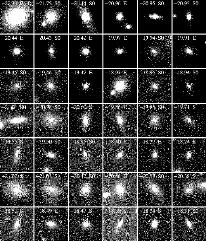
Figure 9: Postage stamp $V$-band images of example members belonging to cluster A85. We show RSGs in the top three rows, with the 18 examples divided into six representative cuts in luminosity starting with the three most luminous, and then decreasing in steps of 0.5 mag from the third brightest cluster RSG. In the bottom four rows we give IBG (rows 4 and 5) and VBG (rows 6 and 7) examples. For the IBGs and VBGs we plot the six brightest in rows 4 and 6, respectively. Similarly, we plot the six faintest (with a minimum luminosity limit of $M_{V}=-18.1+5\log_{10}h$) in rows 5 and 7, respectively. The total $M_{V}-5\log_{10}h$ magnitude and visual classification is given for each galaxy. Each panel is 20 $h^{-1}$ kpc on a side.

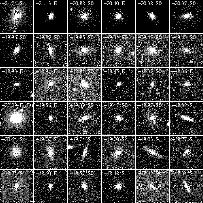
Figure 10: Postage stamp $V$-band images of example members belonging to cluster A496. The representative RSG examples are plotted in rows 1-3 as in Figure 9. We show the six brightest IBGs (row 4) and the twelve brightest VBGs (rows 5 and 6). Each panel is 20 $h^{-1}$ kpc on a side.

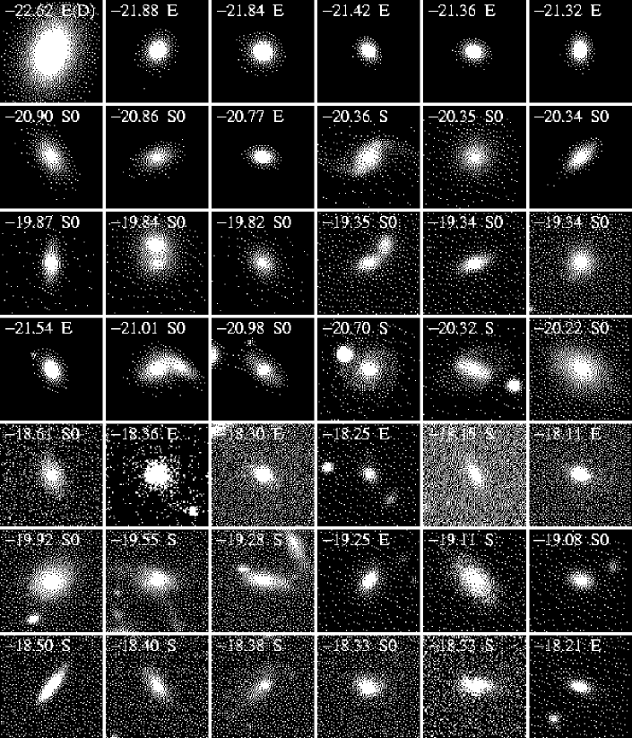
Figure 11: We show example members belonging to cluster A754 following the same format as in Figure 9.

3.3.4 Summary

In this section we have shown that $\sim 20\%$ of the $\geq 0.1L^{\star}$ galaxy population of local Abell clusters, located within $65-85\%$ of the projected virial radius, have blue or moderately blue colors relative to the CMR defined by the red members. In general, the cluster VBGs are spatially, kinematically, and morphologically distinct from the more bound and centrally-concentrated red members with smooth early-type morphologies. In all three clusters, we find the VBGs are more typical of the morphologies of star-forming field galaxies. Moreover, the VBGs tend to lie at projected radii further from the core, with typical velocities displaced from the cluster mean velocity. For two of the three clusters, the VBGs have velocity dispersions that are $\sim\sqrt{2}$ times the dispersion of the red members, which is expected for an infalling, as opposed to virialized, population. These results imply that the bluest galaxies have entered from the field in agreement with the model predictions of Diaferio et al. (2001), and have not yet mixed with the redder (older) cluster galaxies in the core. Our findings are in agreement with other studies that detect a population of nonvirialized, late-type galaxies in clusters (Zabludoff & Franx, 1993; Adami et al., 1998, 2000). The presence of late infall members in low redshift clusters is expected in the hierarchical picture of cluster formation. Identifying these galaxies is invaluable for follow-up studies of what factors might influence the evolution of galaxies in cluster environments. In Paper 1 we concentrate our analysis on quantitative measures of morphology and structure for these late cluster arrivals to further understand their role in the evolution of galaxies in cluster environments.

The spatial, kinematic, and morphological data suggest that an IBG could represent a “transition” object between a more recent arrival with young stars still in abundance (e.g. VBG) and the RSG type now containing only an old stellar population. IBGs make up $5-12\%$ of the galaxies in our cluster sample. Such a population provides evidence for the whereabouts of the blue galaxies once prevalent in rich clusters. The total fraction of present-day cluster IBG$+$VBG populations is representative of cluster VBG fractions at moderate redshift (e.g. $\sim 20\%$).

4 Conclusions

We present a large data base of precise $U,V$ photometry for 637 present-day cluster galaxies, most more luminous than $M^{\star}_{V}+3$. The sample is drawn from square-degree imaging of three nearby ($z<0.06$) Abell clusters: A85, A496, and A754. All galaxies have cluster membership confirmed using spectroscopic redshifts from Christlein & Zabludoff (2003), which removes the need for uncertain field corrections.

To determine the degree to which cluster $(U-V)$ CMRs are uniform in the local universe and thereby constrain galaxy evolution models, we employ a maximum-likelihood technique to analyze the CMR properties of the red galaxies within a projected radius of $1/3R_{200}$ for each cluster in our sample. Using a variety of red galaxy sample selections and $(U-V)$ color measurements, we find that CMRs (defined by slope, intrinsic scatter, and zero point at fixed absolute magnitude $M_{V}=-20+5\log_{10}h$) remain quite uniform, with maximum variations in these properties as follows: 0.047 to 0.112 mag (intrinsic scatter); -0.104 to -0.043 (slope); and 1.34 to 1.45 mag (zero point). We note that the range in zero point color can be explained by systematic photometric error, thus, our results are consistent with homogeneous CMR colors in agreement with Andreon (2003). The range of CMR scatter allows a maximum spread in the formation times of the stellar populations of 5.2 Gyr, with the bulk of the stars forming before $z=1.2$, following the analysis of Bower, Kodama, & Terlevich (1998).

If we limit our analysis to the core red galaxy populations and adopt the same color aperture as used for the Coma Cluster by BLE92, we find that local clusters spanning a range of cluster masses and richnesses have universal CMRs within tighter limits of intrinsic scatter [0.047,0.079] and slope [-0.094,-0.075]. We find that the CMR universality is robust to changes in sample size and sampling radii. Moreover, we show that CMR uniformity extends to $M^{\star}_{V}+3$ and we find no marked change in the slope of the $(U-V)$ relation in contrast with the study of Metcalfe, Godwin, & Peach (1994). Last, we find that CMRs based on colors measured in apertures containing the same fraction of light are inconsistent with flat (i.e. zero slope) as claimed by Scodeggio (2001).

The CMR results that we present here provide an useful benchmark for comparisons with CMRs studied in high redshift clusters using similar rest-frame colors. The variation in CMR scatter we have observed among four nearby Abell clusters (the three in our sample plus Coma; BLE92 Terlevich, Caldwell, & Bower, 2001) is consistent with the values reported in the literature at higher redshifts. This lack of evidence for evolution of the $(U-V)$ CMR scatter suggests, as the narrow CMR scatter among our three clusters does, that the bulk of stars in the red-sequence galaxies formed above $z\sim 1$.

We use the CMR, spatial, kinematic, and morphological data to identify the population of galaxies most recently accreted by the clusters. We first divide each cluster sample into three populations based on $(U-V)$ color relative to the well-defined CMR. The colors of cluster galaxies are likely to depend on their time since arrival (Balogh, Navarro, & Morris, 2000); thus, bluer relative color should correspond to later accretion. We establish the existence of significant numbers ($18-23\%$) of blue and moderately blue galaxies among the luminous ($\geq 0.1L^{\star}$) residents of these Abell clusters. The blue members have spatial, kinematic, and morphological properties that are inconsistent with their red cluster neighbors. In general, we find bluer galaxies prefer the cluster outskirts, avoid the inner regions, have flat and off-center velocity distributions, and have late-type morphologies. These properties provide compelling evidence confirming the more recent arrival nature of members with very blue colors relative to the well-defined CMR. Moreover, the members with intermediate colors are possibly objects in “transition” between more recent arrival VBGs and long-member RSGs. The existence of late cluster arrivals provides the best present-day location to look for evidence of environmental-induced galaxy evolution in cluster environments. To further comment on how the most recent arrival populations fit into the hierarchical picture of cluster galaxy evolution requires more detailed scrutiny (profile model fitting with proper accounting of selection effects) of the blue membership and direct comparison with blue field galaxies, all of which we address in Paper 1.

Appendix A CMR Dependence on Color Aperture Choice

We test how the choice of color aperture (fixed light, identical light fractions) affects the measurement of CMR slope, scatter, and zero point. The use of circular apertures with fixed metric sizes to measure the colors of galaxies does not take into account their different physical sizes. BLE92 noted that CMR slopes will differ between those based on fixed metric and on relative size apertures. Scodeggio (2001) have taken this one step further, arguing that fixed aperture colors introduce a bias in the CMR because early-type galaxies have radial color gradients, with redder centers compared to outskirts (see e.g. Franx, Illingworth, & Heckman, 1989; Peletier et al., 1990). Therefore, galaxies of different intrinsic size (which is related to luminosity) will have different total fractions of their light measured within fixed apertures, which may result in a spurious correlation between galaxy brightness and color. Scodeggio (2001) found that the CMR slope of Coma is significantly diminished to a value consistent with zero, and the intrinsic scatter is much larger, when the BLE92 sample is re-analyzed using half-light apertures. Similarly, Bernardi et al. (2003) found that $(g-r)$ is independent of luminosity for 9000 low-redshift field ellipticals when the total (model-dependent) galaxy light is used to define color. Clearly, measuring colors in apertures containing the same fraction of light is important when attempting to establish the universality of nearby cluster CMRs. In particular, we test whether the use of variable size apertures based on the extent of each galaxy light profile will produce flattened CMRs.

Besides the use of fixed metric apertures, we measure the $(U-V)$ color of all cluster galaxies using two additional circular apertures with radii given by factors of $1\times$ and $2\times$ the half-light radius $r_{\rm hl}$. Our 2D surface brightness fitting (§ 2.4.2) provides PSF-convolved $r_{\rm hl}$ measurements for each galaxy. The use of aperture sizes based on model fit radii introduces an error in color from uncertainties in $r_{\rm hl}$ . We estimate this color error and find it to be negligible in 98% of all cluster galaxies; in the remaining 2% this error is roughly $0.01-0.02$ mag. We note that using such apertures is useful only if the galaxies are resolved. We find 95% (A85), 100% (A496), and 89% (A754) of cluster members to be fully resolved such that twice their half-light size exceeds the common large PSF value we use to degrade the images for color measurements. We require the small fraction of unresolved galaxies to have a limiting aperture diameter equivalent to the large PSF size. We measure colors within the half-light related apertures following the procedure we outline in § 2.5, and we present these measurements electronically (see Table 6).

We apply our CMR analysis to members selected within our default sampling radius of $R_{\rm p}=1/3R_{200}$ and present the results for all aperture color measurements in Table 8 (see rows 2-4, 8-10, and 15-18). $R_{\rm p}$ is the projected cluster-centric radius (relative to the brightest cluster galaxy), and $R_{200}$ is a measure of the virial radius. We do not find dramatic differences between CMR parameters based on fixed or variable aperture colors within a given cluster. In general, the results for the three different apertures are within $2-3\sigma$ of each other. We illustrate the similarity in Figure 12 where we plot the C-M data based on each aperture for cluster galaxies within $1/3R_{200}$. We note that the top panels of Figure 12 show the uniformity of the three cluster CMRs when using fixed metric apertures (§3.2). We find a $2-3\sigma$ (slope measurement error) flattening of the CMR slope when using colors defined in large, roughly total light apertures (i.e. $2r_{\rm hl}$, bottom panels), compared with the fixed metric aperture results (top panels). The slope flattening is greatest for A85 and minimal for A754. Nevertheless, even twice half-light apertures do not remove the CMR slope in any of the three clusters as claimed by Scodeggio (2001).

We note that the only case where the three cluster CMRs are statistically different is found when using half-light colors (middle panels of Figure 12 and rows 3, 9, and 16 of Table 8). Here the slope of A496 is significantly steeper than those of A85 and A754, which are equivalent. A496 is a smaller and less massive cluster than the other two, and it is the closest of the three. It is not clear if these factors contribute to the observed half-light CMR differences; nevertheless, these differences represent the maximum range of CMR slopes that we report.

A small fraction of cluster galaxies in our sample are not resolved (i.e. half-light size less than seeing size, see §2.5). Unresolved galaxies have colors derived from apertures fixed to the seeing size. Therefore, we check whether the fraction of unresolved galaxies included in the CMR analysis could artificially preserve the statistically significant slope we find with half-light aperture colors. We repeat our CMR analysis on the resolved members towards the center of A754, which has the largest fraction of unresolved galaxies. This selection reduces the number of galaxies defining the CMR by $\sim 13\%$ (11/82), yet as shown in Table 8, the best-fit parameters for the smaller sample of 71 resolved red members is an exact match to the CMR including the 11 additional unresolved galaxies. The number of such objects within $1/3R_{200}$ of A85 and A496 are 3 and 0, respectively. Therefore, we assume that their removal will also have no effect on the half-light aperture CMR. We conclude that the seeing of our observations has no effect on our comparisons of fixed and variable size apertures.

Moreover, increased aperture size produces a small systematic blueward shift of the CMR. The difference in CMR zero point from $1r_{\rm hl}$ to $2r_{\rm hl}$ aperture colors is $\Delta(U-V)_{0}=-0.03$ (A85), $\Delta(U-V)_{0}=-0.02$ (A496), and $\Delta(U-V)_{0}=-0.03$ (A754), which corresponds to $\sim 2\sigma$. These differences are roughly $3\sigma$, and thus a real consequence of the color gradients in the presumably early-type (red) galaxies defining the CMR.

Finally, the trends in intrinsic CMR scatter change with color aperture choice are less well defined among the clusters. Increasing the color aperture from $1r_{\rm hl}$ to $2r_{\rm hl}$ results in $0.02$ and $0.01$ mag increases in $\sigma_{\rm CMR}$ for A85 and A496, respectively. Yet, the CMR from larger aperture colors in A754 is roughly 0.01 mag tighter than with the smaller variable aperture. Statistically, these $\sigma_{\rm CMR}$ differences are unimportant ($1-2\sigma$, scatter measurement error). The only significant ($>3\sigma$) change occurs for A85 going from fixed-size to $2r_{\rm hl}$ apertures. For all three clusters we find the minimum intrinsic scatter when using fixed aperture colors.

To summarize, measuring color with galactic half-light radii instead of fixed metric apertures increases the CMR scatter by at most 33% and nearly quadruples the variation in CMR slope among the sample clusters.

Figure 12: Comparison of CMRs based on $(U-V)$ colors using three different aperture diameters: fixed physical size of $3.34$ $h^{-1}$ kpc (top panels), half-light (middle panels), and twice half-light (bottom panels). In each panel we plot the C-M data for cluster galaxies within a projected cluster-centric radius of $1/3R_{200}$. The best-fit CMR (solid line) and its $\pm 1\sigma_{\rm CMR}$ intrinsic dispersion (dashed lines) from our maximum-likelihood fit to the data are shown for each aperture and each cluster (see also Table 8).

Table 1: Cluster Properties

Cluster	$\alpha_{2000}$	$\delta_{2000}$	$l$	$b$	$z$	R	$R_{\rm vir}$	$R_{\rm X}$	$M_{\rm cv}$	$M_{\rm X}$
(1)	(2)	(3)	(4)	(5)	(6)	(7)	(8)	(9)	(10)	(11)
A85	00:41:50.5	-09:18:11.6	116.24	-72.03	0.055	1	1.94	0.7-1.5	9.88	1.3-6.3
A496	04:33:37.8	-13:15:43.5	210.59	-36.49	0.033	1	1.37	0.3-0.6	3.20	0.9-1.9
A754	09:08:32.4	-09:37:46.5	187.67	+24.71	0.055	2	1.32	5.0	4.23	0.6

Note. — Abell catalog designation (1). Epoch J2000.0 celestial (2,3) and Galactic (4,5 in degrees) coordinates of the image center coincident with the brightest cluster galaxy (a cD galaxy for clusters A85 and A496; a D class galaxy in the case of A754). The mean cluster redshift (6). The Abell richness (7), which is defined by Abell (1958) as the number of galaxies $N_{\rm gal}$ in a cluster with $m\leq m_{3}+2$, where $m_{3}$ is the third brightest member. The richness values reported here correspond to $50\leq N_{\rm gal}\leq 79$ (R=1), and $80\leq N_{\rm gal}\leq 129$ (R=2). From Girardi et al. (1998), the virial (8) and X-ray derived (9) radii in units of $h^{-1}$ Mpc , and the virial (10) and X-ray (11) masses in units of $10^{14}h^{-1}$ M$\sun$ within corresponding radii.

Table 2: Cluster Observations

Cluster	Date	Filter	Camera	$t_{\rm exp}$	Seeing	$\sec{z}$	FOV	scale	Conditions
(1)	(2)	(3)	(4)	(5)	(6)	(7)	(8)	(9)	(10)
A85	Nov. 28, 1997	$V$	MOS1	$5\times 600$	1.2	1.33-1.36	2.7	0.32	photometric
	Jan. 04, 2001	$U$	MOS2	$5\times 600$	1.4	1.41-1.58			photometric
A496	Nov. 25, 1997	$V$	MOS1	$5\times 600$	1.3	1.42-1.47	1.6	0.19	non-photometric
	Nov. 27, 1997	$V$	MOS1	$1\times 300$	1.2	1.43			photometric
	Jan. 04, 2001	$U$	MOS2	$5\times 720$	1.3	1.42-1.44			photometric
A754	Nov. 28, 1997	$V$	MOS1	$5\times 480$	1.1	1.34-1.36	2.7	0.31	photometric
	Nov. 28, 1997	$V$	MOS1	$1\times 300$	1.1	1.34			photometric
	Jan. 3, 2000	$U$	MOS2	$3\times 720$	2.4	1.37-1.43			poor seeing
	Jan. 4, 2000	$U$	MOS2	$5\times 720$	2.0	1.34-1.39			photometric

Note. — For each cluster observation we give the date (2), filter (3), and detector (4). The exposure time (5) is given by the number of exposures multiplied by the duration of each integration. Single exposures were obtained for calibration during photometric conditions. The average seeing FWHM (6) in arcseconds and the range of airmass (7) given as $\sec z$ for a set of exposures. For each cluster we provide the physical scale of the square-degree diameter field of view (8; FOV) in units of $h^{-1}$ Mpc, and the physical pixel scale (9) in units of $h^{-1}$ kpc pix^-1. We note the conditions during observations in (10).

Table 3: Final Cluster Image Properties

Cluster	Filter	$\left<{\rm bkg}\right>$	$\sigma_{\rm bkg}$	$\tilde{t}_{\rm exp}$	$\tilde{X}$	$zp_{\rm eff}$
(1)	(2)	(3)	(4)	(5)	(6)	(7)
A85	V	45.52	1.61	600	1.33	26.894
	U	17.75	1.88	600	1.41	26.629
A496	V	37.67	1.25	300	1.42	26.162
	U	18.17	1.84	720	1.44	26.814
A754	V	31.09	1.36	480	1.34	26.651
	U	22.74	1.56	720	1.34	26.857

Note. — Properties of each fully reduced cluster image are passband (2), average background level in adu (3), RMS pixel-to-pixel noise in adu (4), effective exposure time in seconds (5), effective airmass (6), and effective zero point (7).

Table 4: Photometric Transformation Equation Coefficients

Date	Filter	Scope/Detector	$N_{\rm stars}$	fit RMS	$zp$	$\alpha$	$\beta$
(1)	(2)	(3)	(4)	(5)	(6)	(7)	(8)
Nov. 27, 1997	V	0.9-meter/MOS1	44	0.029	$20.161\pm 0.012$	$-0.135\pm 0.006$	$-0.003\pm 0.008$
Nov. 28, 1997	V	0.9-meter/MOS1	34	0.029	$20.063\pm 0.026$	$-0.086\pm 0.014$	$0.009\pm 0.008$
Jan. 4, 2000	U	0.9-meter/MOS2	112	0.058	$20.287\pm 0.028$	$-0.428\pm 0.016$	$-0.018\pm 0.012$

Note. — For each night that photometric standards were observed we give the date (1), filter (2), and scope plus detector system (3). The best-fit solution to the transformation equation for photometric calibration was achieved using the given number of unique standard stars (4), with an RMS in magnitudes (5), and with best-fit coefficients and uncertainties given for the zero point (6), airmass (7), and color (8) terms.

Table 5: Cluster Image Source Catalogs

Cluster	Image	$N_{\rm good}$	$m_{\rm min}$	$N_{\rm min}$	$N_{\rm ext}$	$N_{\rm gal}^{U,V}$
(1)	(2)	(3)	(4)	(5)	(6)	(7)
A85	$V$	4128	20.5	2786	1448
	$U$	1574	20.7	1453
	total					455
A496	$V$	3301	20.5	3063	730
	$U$	2183	21.0	2043
	total					315
A754	$V$	8786	21.0	7578	2142
	$U$	3924	20.5	3451
	total					547

Note. — Breakdown of cluster source catalogs. The image catalog passband or ‘total’, which denotes the final $U$ and $V$ combined catalog, is designated in (2). Total number of ‘good’ sources (3) after the removal of saturated, bad, and edge objects. Empirical magnitude limit (4) and corresponding number of sources brighter than $m_{\rm min}$ (5). Number of ‘extended’ sources in the $V$-band image (6), and final quantity of $V$-band galaxies with $U$ counterparts (7).

Table 6: Example of the Catalog of Cluster Galaxy Photometry

Galaxy	$z$	$M_{V}-5\log_{10}h$	$(U-V)_{3.34}$	$(U-V)_{\rm hl}$	$(U-V)_{\rm 2hl}$	$E(B-V)$	$k_{V}$	$k_{(U-V)}$
(1)	(2)	(3)	(4)	(5)	(6)	(7)	(8)	(9)
A85.004150$-$091811	0.055	$-22.73\pm 0.03$	$1.44\pm 0.03$	$1.42\pm 0.03$	$1.38\pm 0.03$	0.04	-0.10	-0.08
A85.003959$-$092604	0.057	$-18.61\pm 0.05$	$0.65\pm 0.03$	$0.67\pm 0.03$	$0.83\pm 0.03$	0.03	-0.10	-0.08
A85.004005$-$090303	0.056	$-20.35\pm 0.03$	$1.66\pm 0.03$	$1.61\pm 0.03$	$1.58\pm 0.03$	0.03	-0.10	-0.08
A85.004013$-$085957	0.055	$-19.26\pm 0.04$	$1.46\pm 0.03$	$1.46\pm 0.03$	$1.37\pm 0.03$	0.03	-0.10	-0.08
A85.004018$-$085631	0.052	$-18.33\pm 0.08$	$1.30\pm 0.04$	$1.30\pm 0.04$	$1.26\pm 0.03$	0.03	-0.09	-0.07
A496.043256$-$133639	0.038	$-20.63\pm 0.07$	$0.65\pm 0.05$	$0.67\pm 0.05$	$0.70\pm 0.05$	0.18	-0.07	-0.06
A496.043258$-$131218	0.036	$-19.25\pm 0.05$	$1.19\pm 0.03$	$1.16\pm 0.03$	$1.21\pm 0.03$	0.08	-0.07	-0.05
A496.043259$-$131820	0.034	$-17.83\pm 0.10$	$1.12\pm 0.04$	$1.14\pm 0.04$	$1.12\pm 0.04$	0.10	-0.06	-0.05
A496.043300$-$131600	0.037	$-20.12\pm 0.06$	$1.45\pm 0.04$	$1.44\pm 0.04$	$1.41\pm 0.04$	0.09	-0.07	-0.05
A496.043300$-$134232	0.035	$-19.39\pm 0.09$	$1.04\pm 0.06$	$0.90\pm 0.06$	$0.80\pm 0.06$	0.23	-0.06	-0.05
A754.090645$-$093424	0.060	$-17.74\pm 0.08$	$0.22\pm 0.03$	$0.21\pm 0.03$	$0.21\pm 0.03$	0.07	-0.11	-0.08
A754.090803$-$100214	0.054	$-20.09\pm 0.05$	$1.65\pm 0.04$	$1.62\pm 0.04$	$1.61\pm 0.04$	0.08	-0.10	-0.08
A754.090806$-$092600	0.054	$-18.94\pm 0.05$	$0.77\pm 0.03$	$0.79\pm 0.03$	$0.74\pm 0.03$	0.06	-0.10	-0.08
A754.090806$-$092713	0.051	$-19.02\pm 0.04$	$0.54\pm 0.02$	$0.58\pm 0.02$	$0.58\pm 0.02$	0.06	-0.09	-0.07
A754.090807$-$100410	0.050	$-18.07\pm 0.08$	$1.38\pm 0.04$	$1.41\pm 0.05$	$1.38\pm 0.04$	0.09	-0.09	-0.07

Note. — The full catalog is available electronically. Galaxy identification based on cluster designation and J2000.0 celestial coordinates (1). Rest-frame $V$-band total absolute magnitude (2). Rest-frame $(U-V)$ colors measured within three circular apertures: fixed size corresponding to $3.34$ $h^{-1}$ kpc at distance to parent cluster (3); variable sizes (see Appendix A) corresponding to half-light (4) and twice half-light (5) galaxy diameters. The photometry is calibrated to Johnson $U$ and $V$ magnitudes on the Landolt (1992) system, and each measurement includes formal random errors.

Table 7: Cluster Membership Results

Cluster	$\left<cz\right>_{\rm clus}$	$\sigma_{\rm clus}$	$DM$	$R_{200}$	$N_{z}$	$N_{\rm mem}$	$N_{\rm non}$	$N_{\rm miss}$	$\theta_{\rm sep}$
(1)	(2)	(3)	(4)	(5)	(6)	(7)	(8)	(9)	(10)
A85	$16607\pm 60$	$993\pm 53$	36.184	1.67	331	180 (0.4/0.5/0.1)	80	71 (27)	1.15
A496	$9910\pm 48$	$728\pm 36$	35.030	1.24	225	146 (0.2/0.6/0.2)	26	53 (33)	0.90
A754	$16369\pm 47$	$953\pm 40$	36.158	1.61	415	311 (0.3/0.6/0.1)	50	54 (24)	1.66

Note. — For each cluster (1), the mean recessional velocity (2) and internal velocity dispersion (3), in units of km $s^{-1}$, are given from the spectroscopic survey of Christlein & Zabludoff (2003). The resultant cosmological distance modulus assuming $h=1$ (4), and $R_{200}$ (5) in units of $h^{-1}$ Mpc in our adopted cosmology, which is an estimate of the cluster virial radius defined to encompass a density that is 200 times the critical density at a given redshift (Finn, Zaritsky, & McCarthy, 2004). The total number of redshifts within our images (6), which is divided into the following quantities: members meeting the membership criteria (see text) with $U,V$ image source counterparts (7); non-members with $U,V$ image sources (8); and spectroscopic sources without image matches (9), with the number of unmatched member redshifts given in parentheses. The average coordinate separations (10) between the imaging and spectroscopic matchups. Within the parentheses of column (7) we give the relative fractions of bright member galaxies ($\geq 0.1L^{\star}$) split into three basic visual morphology types (E/S0/S+Irr).

Table 8: Best-Fit CMR Analysis Results

Cluster	Ap	$R_{\rm p}/R_{200}$	$N_{\rm fit}$	$(U-V)_{0}$	$\sigma_{\rm CMR}$	$d(U-V)/dM_{V}$	$\mathcal{L}_{\rm max}$
(1)	(2)	(3)	(4)	(5)	(6)	(7)	(8)
A85	1	$0.30(0.50)$	48/ 62	$1.38\pm 0.01$	$0.079\pm 0.010$	$-0.075\pm 0.012$	49.8
A85	1	$0.33(0.56)$	53/ 67	$1.38\pm 0.01$	$0.076\pm 0.008$	$-0.078\pm 0.010$	55.9
A85	2	$0.33(0.56)$	54/ 67	$1.37\pm 0.01$	$0.090\pm 0.011$	$-0.054\pm 0.012$	48.4
A85	3	$0.33(0.56)$	55/ 67	$1.34\pm 0.02$	$0.112\pm 0.010$	$-0.056\pm 0.014$	40.8
A85	1	$0.37(0.60)$	60/ 78	$1.39\pm 0.01$	$0.074\pm 0.009$	$-0.077\pm 0.010$	65.7
A496	1	$0.25(0.31)$	45/ 50	$1.35\pm 0.01$	$0.060\pm 0.009$	$-0.077\pm 0.010$	53.2
A496	1	$0.30(0.37)$	50/ 60	$1.35\pm 0.01$	$0.047\pm 0.007$	$-0.087\pm 0.008$	69.3
A496	1	$0.33(0.41)$	60/ 71	$1.35\pm 0.01$	$0.053\pm 0.009$	$-0.082\pm 0.008$	77.4
A496	2	$0.33(0.41)$	60/ 71	$1.36\pm 0.01$	$0.055\pm 0.009$	$-0.104\pm 0.009$	77.1
A496	3	$0.33(0.41)$	60/ 71	$1.34\pm 0.01$	$0.065\pm 0.009$	$-0.073\pm 0.009$	69.1
A496	1	$0.37(0.46)$	70/ 80	$1.35\pm 0.01$	$0.053\pm 0.008$	$-0.081\pm 0.007$	87.4
A496	1	$0.50(0.60)$	91/111	$1.35\pm 0.01$	$0.055\pm 0.007$	$-0.089\pm 0.010$	111.7
A754	1	$0.20(0.32)$	52/ 58	$1.42\pm 0.01$	$0.055\pm 0.008$	$-0.089\pm 0.008$	68.9
A754	1	$0.30(0.48)$	75/ 83	$1.42\pm 0.01$	$0.050\pm 0.009$	$-0.093\pm 0.009$	105.4
A754	1	$0.33(0.54)$	86/ 95	$1.42\pm 0.01$	$0.056\pm 0.007$	$-0.093\pm 0.007$	111.0
A754	2	$0.33(0.54)$	89/ 95	$1.40\pm 0.01$	$0.083\pm 0.009$	$-0.069\pm 0.010$	89.0
A754	$2^{a}$	$0.33(0.54)$	77/ 82	$1.40\pm 0.01$	$0.084\pm 0.009$	$-0.071\pm 0.011$	76.5
A754	3	$0.33(0.54)$	89/ 95	$1.37\pm 0.01$	$0.075\pm 0.009$	$-0.080\pm 0.008$	95.9
A754	1	$0.37(0.60)$	95/107	$1.43\pm 0.01$	$0.061\pm 0.008$	$-0.094\pm 0.008$	116.7

Note. — Cluster designation (1). Aperture type (2) for $(U-V)$ color measurement: 1 = fixed size corresponding to $3.34$ $h^{-1}$ kpc at distance to cluster; 2 = variable size corresponding to half-light galaxy diameter; 3 = variable size corresponding to twice half-light galaxy diameter. The projected cluster-centric radius in terms of $R_{200}$ is given in (3), and in units of $h^{-1}$ Mpc in parentheses. For comparison, the Coma cluster has $R_{200}=1.76h^{-1}$ Mpc based on $z=0.022$ and $\sigma_{\rm clus}=1008$ km $s^{-1}$ from Struble & Rood (1999). Within projected radius $R_{\rm p}$, the number of galaxies used in the final fit (after outlier clipping, see text) relative to the total number are given in (4). The best-fit CMR parameters from our maximum likelihood analysis are zero point (5), intrinsic scatter (6), and slope (7), and there associated uncertainties. The maximum likelihood for each fit is given in (8).

Table 9: Color-magnitude Galaxy Population Breakdown

Cluster	$L/L^{\star}$	$N_{\rm mem}$	$N_{\rm RSG}$	$N_{\rm IBG}$	$N_{\rm VBG}$
(1)	(2)	(3)	(4)	(5)	(6)
A85	$\geq 0.1$	164	126 (56,68,2)	14 (4,7,3)	24 (5,6,13)
	$<0.1$	16	4 (4,0,0)	3 (1,1,1)	9 (3,2,4)
A496	$\geq 0.1$	101	83 (18,56,9)	6 (0,5,1)	12 (1,1,10)
	$<0.1$	45	29 (14,5,10)	1 (1,0,0)	15 (0,0,15)
A754	$\geq 0.1$	281	227 (68,146,13)	35 (9,18,8)	19 (2,4,13)
	$<0.1$	30	21 (17,3,1)	4 (3,0,1)	5 (1,0,4)

Note. — Breakdown of color-based populations for each cluster divided into two subsamples: brighter than $0.1L^{\star}$ ($M_{V}=-18.1+5\log_{10}h$) and fainter. For each luminosity bin (2), we give the total number of cluster members (3) split into RSG (4), IBG (5), and VBG (6) types. We give the number per three visual morphology types (E,S0,S+Irr) in the parentheses in each column.

Table 10: Statistical Test Results for Cluster Kinematics

Cluster	C-M Pop.	$\left<\Delta v\right>$	$\sigma$	$N$	K-S test	F-test	t-Test
(1)	(2)	(3)	(4)	(5)	(6)	(7)	(8)
A85	RSG	-102	908	130
	VBG	+656	1260	33	$>99.9\%$	98.9%	99.8%
	IBG	+262	1210	17	70.4%	91.6%	99.8%
A496	RSG	+165	727	112
	VBG	-245	1050	17	99.3%	99.1%	93.6%
A754	RSG	+21	958	248
	VBG	-425	969	24	93.9%	0.1%	97.0%
	IBG	-3	929	39	0.1%	0.1%	0.1%

Note. — Results of tests for differences between the kinematic distributions of cluster RSGs compared with the blue galaxy (VBG and IBG) populations. For the color-selected galaxy populations (2) of each cluster, we give the mean (3) and standard deviation (4) of the relative velocity distributions in km s^-1. The number of galaxies in each sample is given in (5). In (6) we tabulate the K-S test probability that the blue galaxy population is not drawn from the same parent sample as the RSGs. We give the F-test significance for differences between sample variances in (7), and likewise the T-test significance for sample mean differences in (8). We note that for cases where the sample variance is different at the $>90\%$ level, we use the “unequal variances” version of the T-test (see text). As a result of the small number of IBGs in A496 ($N=7$), we do not test for differences between the kinematics of this population and the cluster’s RSGs.

References

- Abadi, Moore, & Bower (1999) Abadi, M. G., Moore, B., & Bower, R. G. 1999, MNRAS, 308, 947
- Abell (1958) Abell, G. O. 1958, ApJS, 3, 211
- Abraham et al. (1996) Abraham, R. G., Smecker-Hane, T. A., Hutchings, J. B., Carlberg, R. G., Yee, H. K. C., Ellingson, E., Morris, S., Oke, J. B., & Rigler, M. 1996, ApJ, 471, 694
- Adami et al. (1998) Adami, C., Biviano, A., & Mazure, A. 1998, A&A, 331, 439
- Adami et al. (2000) Adami, C., Holden, B. P., Castander, F. J., Mazure, A., Nichol, R. C., & Ulmer, M. P. 2000, A&A, 362, 825
- Andreon (2003) Andreon, S. 2003, A&A, 409, 37
- Balogh & Morris (2000) Balogh, M. L., & Morris, S. L. 2000, MNRAS, 318, 703
- Balogh, Navarro, & Morris (2000) Balogh, M. L., Navarro, J. F., & Morris, S. L. 2000, ApJ, 540, 113
- Bekki (1998) Bekki, K. 1998, ApJ, 502, L133
- Bekki, Couch, & Shioya (2002) Bekki, K., Couch, W. J., & Shioya, Y. 2002, ApJ, 577, 651
- Bernardi et al. (2003) Bernardi, M., et al. 2003, AJ, 125, 1882
- Bertin & Arnouts (1996) Bertin, E., & Arnouts, S. 1996, A&AS, 117, 39
- Bicker et al. (2002) Bicker, J., Fritze-von Alvensleben, U., & Fricke, K. J. 2002, A&A, 387, 412
- Binney & Merrifield (1998) Binney, J., & Merrifield, M. 1998, Galactic Astronomy, Princeton University Press
- Boroson et al. (1994) Boroson, T., Reed, R., Wong, W.-Y., & Lesser, M. P. 1994, SPIE, 2198, 877
- Bower, Kodama, & Terlevich (1998) Bower, R. G., Kodama, T., & Terlevich, A. 1998, MNRAS, 299, 1193
- Bower, Lucey, & Ellis (1992a) Bower, R. G., Lucey, J. R., & Ellis, R. S. 1992, MNRAS, 254, 589 (BLE92)