The Microarcsecond Sky and Cosmic Turbulence

Abstract

Radio waves are imprinted with propagation effects from ionized media through which they pass. Owing to electron density fluctuations, compact sources (pulsars, masers, and compact extragalactic sources) can display a wide variety of scattering effects. These scattering effects, particularly interstellar scintillation, can be exploited to provide superresolution, with achievable angular resolutions ($\mathbin{\lower 3.0pt\hbox{$\hbox to0.0pt{\raise 5.0pt\hbox{$\char 60\relax$}\hss}\mathchar 29208\relax$}}1\,\mu$arc sec) far in excess of what can be obtained by very long baseline interferometry on terrestrial baselines. Scattering effects also provide a powerful sub-AU probe of the microphysics of the interstellar medium, potentially to spatial scales smaller than 100 km, as well as a tracer of the Galactic distribution of energy input into the interstellar medium through a variety of integrated measures. Coupled with future $\gamma$-ray observations, SKA observations also may provide a means of detecting fainter compact $\gamma$-ray sources. Though it is not yet clear that propagation effects due to the intergalactic medium are significant, the SKA will either detect or place stringent constraints on intergalactic scattering.

1 Introduction

All radio observations of Galactic and extragalactic objects are conducted while viewing these objects through the Galaxy’s interstellar medium (ISM). Dispersion of pulsar signals and optical observations, particularly of the H$\alpha$ emission line [28], indicate that the interstellar medium contains a diffuse ionized component in addition to classical H ii regions. This interstellar plasma occupies a significant fraction ($\sim 0.2$) of the volume of the ISM, and the energy required to keep it ionized is considerable, roughly 15–20% of the luminosity of all of the O stars in the Galaxy. The interstellar plasma is also known as the Warm Ionized Medium (WIM) or the Diffuse Ionized Gas (DIG). Significantly for the SKA, the interstellar plasma will produce observable effects on every line of sight over at least a fraction of the entire proposed operating frequency range.

The SKA can allow unprecedented use of interstellar scattering and interstellar scintillation (ISS) for study of sources and intervening media:

• Resolving source structure on angular scales $\mathbin{\lower 3.0pt\hbox{$\hbox to0.0pt{\raise 5.0pt\hbox{$\char 60\relax$}\hss}\mathchar 29208\relax$}}10^{-6}$ arcsec will probe the inner jet regions in active galactic nuclei and individual source regions in pulsar magnetospheres. Astrophysically, such observations may be crucial to an understanding of acceleration of particles in these and other kinds of sources. The SKA’s sensitivity over a wide range of frequencies is needed to exploit the resolving power of ISS.

• Probing microturbulence in the ionized ISM through sampling of scattering phenomena along large numbers ($\mathbin{\lower 3.0pt\hbox{$\hbox to0.0pt{\raise 5.0pt\hbox{$\char 62\relax$}\hss}\mathchar 29208\relax$}}10^{4}$) lines of sight. The microturblence plays important roles in the energetics of the ISM and in the propagation of cosmic rays in the Galaxy’s magnetic field.

• Probing the intergalactic medium (IGM) through detection of angular broadening in excess of that expected from foreground Galactic gas. The SKA allows angular broadening measurement of large samples of active galactic nuclei (e.g., $10^{6}$ lines of sight) that will map out contributions from individual intervening galaxies, galaxy clusters, Ly-$\alpha$ clouds, and from a pervasive but clumpy ionized IGM that comprises most of the baryonic matter in the Universe.

Radio-wave scattering from density fluctuations in the interstellar plasma offers both a means of characterizing the ISM on sub-AU scales as well as a powerful probe of source structure. In the remainder of this section, we describe observable effects and astrophysical measures to quantify the interstellar plasma. Subsequent sections discuss interstellar scintillation and superresolution of source structure (§2), the microphysics of the interstellar plasma (§3), interstellar scattering as a means to measure distances (§4), the possibility of intergalactic scattering (§5), the potential impact of scintillations on SKA observations (§6), and key observations to be carried out with the SKA (§7).

1.1 Observable Effects

The phase of a radio wave of wavelength $\lambda$ after having propagated through a plasma is

$$\phi=\int dz\,\lambda\,r_{e}n_{e}(z),$$ (1)

where $r_{e}$ is the classical electron radius and $n_{e}$ is the plasma density. Soon after the discovery of pulsars, it became clear that their signals were displaying intensity scintillations (e.g., [60]), akin to the scintillation of star light at optical wavelengths viewed through the Earth’s atmosphere. Intensity scintillations result from constructive and destructive interference and occur if the phase of the wave has been perturbed during its propagation with structure on small transverse scales. As eqn. (1) shows, phase perturbations imply that the propagating wave has been scattered by interstellar electron density fluctuations. Figure 1 illustrates the relevant geometry.

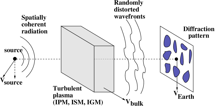
Figure 1: Geometry of radio-wave scattering in the ISM that is responsible for a variety of seeing and scintillation effects.

Since the detection of pulsar intensity scintillations, a rich variety of additional interstellar scattering observables has been recognized. These include [59, 15]:

Intensity Scintillation:

The original indication of interstellar density fluctuations, intensity scintillations have been detected not only from pulsars but potentially also from active galactic nuclei (AGN) and from masers.

Angular broadening (“seeing”):

Compact radio sources, both Galactic and extragalactic, show angular broadening by amounts ranging from $\mathbin{\lower 3.0pt\hbox{$\hbox to0.0pt{\raise 5.0pt\hbox{$\char 60\relax$}\hss}\mathchar 29208\relax$}}1$ mas to 1 arcsec at 1 GHz, depending on the distance and direction. The angular smearing scales approximately as $\nu^{-2}$.

Pulse broadening:

Multipath propagation causes a multiplicity of arrival times, usually seen as an exponential-like “tail” to pulses from pulsars.

Angular wandering:

Focussing and defocussing of rays by AU-scale structures can cause apparent shifts in source positions.

Pulse time of arrival (TOA) fluctuations:

Changes in geometry caused by proper motions of a pulsar and intervening material induce variations in the amount of plasma along the line of sight. Also, variable scattering causes variable arrival times.

Spectral Broadening:

Broadening of narrow spectral lines from a combination of scattering and time-variable geometry. This effect is very small in the ISM ($\mathbin{\lower 3.0pt\hbox{$\hbox to0.0pt{\raise 5.0pt\hbox{$\char 60\relax$}\hss}\mathchar 29208\relax$}}1$ Hz) and has not been found because there are no known sources that produce spectral lines narrow enough for this effect to be significant. It has been measured from spacecraft viewed through the interplanetary medium [31], and, if extraterrestrial transmitters are ever found, it may be important for them.

1.2 Integrated Measures

As we discuss in more detail below, radio measurements provide four integrals involving the electron density and magnetic field. Differential arrival times from pulsars provide the dispersion measure,

$${\rm DM} = \int_{0}^{D}ds\,{n_{e}}(s)\quad({\rm pc\,cm^{-3}}),$$ (2)

(for $D$ in pc and $n_{e}$ in cm^-3). A magnetized plasma produces Faraday rotation, which is described by the rotation measure,

$${\rm RM} = \frac{e^{3}}{2\pi m_{e}^{2}c^{4}}\int_{0}^{D}ds\,{n_{e}}{B_{\parallel}},$$ (3)

$$= 0.81\,\mathrm{rad\,m^{-2}}\,\int_{0}^{D}ds\,{n_{e}}{B_{\parallel}},$$

the integral of the magnetic field component parallel to the line-of-sight ${B_{\parallel}}$ (in $\mu$G) and which is sensitive to the correlation of electron density and magnetic field.

The emission measure can be measured from recombination line and free-free absorption or emission observations in the radio and observations of H$\alpha$ in the optical

$${\rm EM}=\int_{0}^{D}ds\,{n_{e}}^{2}\quad({\rm pc\,cm^{-6}})$$ (4)

(for $D$ in pc and $n_{e}$ in cm^-3).

As we discuss below, the density fluctuations responsible for interstellar scattering can be described in terms of a power spectrum. The scattering measure is the integral of ${C_{n}^{2}}$, the coefficient of the wavenumber spectrum for electron-density fluctuations, ${\delta n_{e}}$,

$${\rm SM}=\int_{0}^{D}ds\,{C_{n}^{2}}(s)\quad(\mathrm{kpc\,m}^{-20/3}).$$ (5)

Cordes et al. [16] give relations between DM, SM, and EM.

Finally, diffuse $\gamma$-ray emission is given by

$$I_{\gamma}=\int ds\,n_{n}(s)q_{\gamma}(s),$$ (6)

where $n_{n}$ is the nucleon density which is dominated by the hydrogen number density $n_{H}$, i.e., H ii, H i, and H₂; $q_{\gamma}$ is the gamma-ray emissivity per nucleon, which is proportional to the cosmic-ray density; and $ds$ is a path-length element along the line of sight. Although not yet exploited, combining future radio and $\gamma$-ray observations may allow fluctuations in $q_{\gamma}$, resulting from magnetic field fluctuations, to be traced.

From large sets of measurements of these measures, but, in particular DM, SM, and RM, the spatial distribution and volume filling factor of the electron density and its fluctuations, e.g., as parameterized by a wavenumber spectrum for quantities such as ${\delta n_{e}}$ and $\delta{B_{\parallel}}$, can be probed as can the large-scale structure and fluctuations in the magnetic field.

2 Interstellar Scintillation (ISS) and Superresolution

“Stars twinkle but planets do not” is an exploitation of how superresolution is obtained via propagation through a turbulent medium. Planets do not twinkle, even though their reflected light travels through the same turbulent atmosphere as does starlight, because their angular diameters are so large as to quench the scintillations. Comparison of a twinkling star and non-twinkling planet obtains constaints on their angular diameters that are roughly an order of magntiude better than the nominal resolution of the human eye. “Pulsars twinkle but AGNs do not” is the interstellar equivalent, albeit that interstellar radio-wave scintillation shows a much richer range of scintillation effects than does atmospheric optical scintillation.

Radio astronomy has a long history of exploiting propagation effects to constrain source diameters. Pulsars were discovered as a result of a program of interplanetary scintillation observations to measure source diameters at low frequencies. In an analogous fashion, the SKA can exploit interstellar scintillation (ISS) to obtain source structure information on angular scales far smaller than can be obtained by very long baseline interferometry (VLBI) on terrestrial baselines.

2.1 Scintillation Regimes

The Fresnel scale, $R_{F}\sim\sqrt{\lambda D}$, defines the approximate spatial scale over which an observer receives radiation. The character of ISS or the scintillation regime depends upon the rms phase imposed by density fluctuations over the Fresnel scale. If the rms phase is comparable to or less than 1 radian, the weak scintillation regime is obtained; if the rms phase is greater than 1 radian, the strong scintillation regime is obtained. Figure 2 summarizes these ISS regimes over a frequency range appropriate to the SKA.

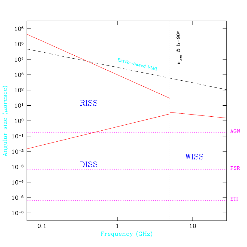
Figure 2: Scintillation regimes over the frequency range appropriate to the SKA. The abscissa is the frequency, and the ordinate is a characteristic angular diameter. Horizontal dashed lines indicate intrinsic angular diameters appropriate for various classes of sources (AGN, pulsars, and ET transmitters). Various regions are labelled as to whether a source of a given angular diameter observed at a given frequency could display one of the forms of ISS. The vertical dashed line shows the approximate frequency for the transition between strong and weak ISS for observations toward a Galactic latitude of $|b|=90^{\circ}$. The sloping line near the top of the plot indicates the angular resolution limit for VLBI observations over terrestrial baselines.

Weak Interstellar Scintillation (WISS)

A geometrical optics approach can be adopted, and the phase variations result in modest focussing and defocussing of the radiation. The normalized rms intensity variation or scintillation index is less than unity. A source will display WISS if its angular diameter is comparable to or less than an isoplanatic angle of approximately $R_{F}/D$. WISS typically occurs for sources observed over modest path lengths at frequencies of order 5 GHz and produce intensity fluctuations on time scales of order hours to days and on frequency scales that are comparable to the radio wave frequency.

In the strong scintillation regime, the power spectrum of the intensity fluctuations bifurcates, and two kinds of ISS are observed.

Diffractive intensity scintillations (DISS)

An rms phase of unity is obtained on the diffractive scale $l_{d}$, with $l_{d}\ll R_{F}$. Consequently, there are many independent phase variations within the Fresnel scale, strong constructive and destructive interference results (Figure 3), and the (diffractive) scintillation index saturates at unity. In general, a wave optics approach must be adopted. A source will display DISS only if its angular diameter is comparable to or less than an isoplanatic angle of approximately $l_{d}/D$. This is a stringent requirement, as $l_{d}\sim 10^{9}$ cm and $l_{d}/D\sim 10^{-6}$ arcseconds for typical path lengths through the ISM at meter wavelengths and only pulsars are known to display DISS. DISS is observed on times scales $\sim 100$ s and frequency scales $\sim 1$ MHz, though these scales are highly dependent on frequency, direction, and source distance and velocity. The diffracted radiation has an angular spectrum with a characteristic scale of order $\theta_{d}\sim\lambda/\ell_{d}$.

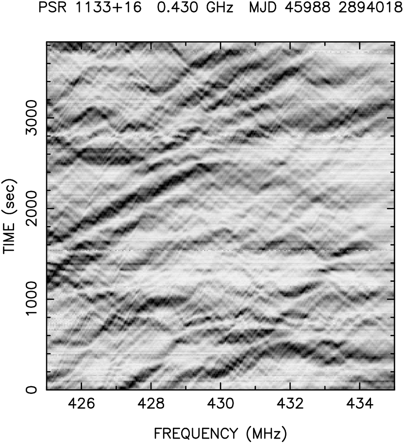
Figure 3: Dynamic spectrum for the pulsar PSR B1133$+$16 in the strong scintillation regime. The abscissa is the observing frequency, the ordinate is time, and the gray scale shows the pulsar intensity, with dark areas indicating strong intensity. The time-frequency structure is an illustration of superresolution as it includes fringes associated with interference between radiation arriving in small discrete bundles of ray paths. The data are from the Arecibo Observatory (JMC, unpublished).

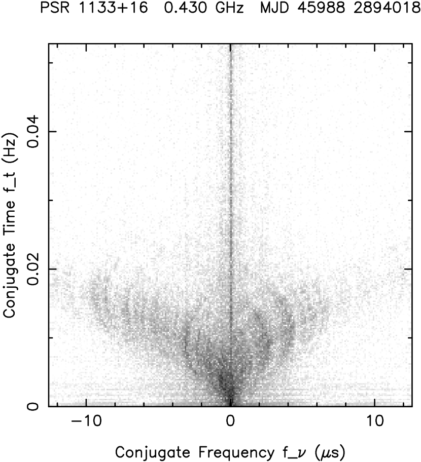
Figure 4: The 2D power spectrum (“secondary spectrum”) of the dynamic spectrum in Figure 3. The axes are conjugate to those in the dynamic spectrum and thus have reciprocal units. The gray scale maps 5 orders of magnitude in going from black (brightest) to white (dimmest). The vertical feature along the $f_{t}$ axis at $f_{\nu}=0$ is caused by broadband, pulse to pulse variations intrinsic to the pulsar. Other features include slanted and arc-like structures (discovered in [69]) caused by interference between radiation contributions arriving at widely spaced angles (wide compared to the rms or characteristic scattering angle). These features can be used to resolve pulsar magnetospheres and fine structure in other sources that show DISS. The resolving power of the phenomenon is comparable to that of an interferometer whose baseline equals the projected separation of the rays at the distance of the effective scattering screen. The weak arcs therefore provide greater angular resolution than do the more prominent features in dynamic spectra that are related to the rms scattering angle. To use arcs for this purpose, dynamic spectra and their secondary spectra could be analyzed for different pulse components of a pulsar. Alternatively, a single secondary spectrum could be synthesized that takes an overall finite source size into account. The resolving power is in the vicinity of 0.1–10 $\mu$s.

Refractive intensity scintillation (RISS)

Large scale focusing and defocusing of the radiation occurs over the refractive scale, $\ell_{r}\sim D\theta_{d}$, implying the well known relation, $\ell_{r}\ell_{d}\sim R_{F}^{2}$. Geometrical optics are sufficient, similar to WISS, and the (refractive) scintillation index is less than unity. The requirements to show RISS are more modest than for DISS as the source diameter must be comparable to or less than $\ell_{r}/D\sim\theta_{d}$ and $\theta_{d}\sim 1$ mas at 1 GHz. In addition to pulsars, active galactic nuclei (AGN) and masers have exhibited RISS.

Finally, although AGN are typically too extended to display DISS, their angular diameters can be comparable to $\theta_{d}$ meaning that they can display angular broadening and be used to probe interstellar density fluctuations.

2.2 Superresolution Using DISS

DISS is caused by multipath scattering of radio waves from small-scale density irregularities in the interstellar plasma. It is sensitive to intrinsic sizes of radiation sources in much the same way that optical scintillation from atmospheric turbulence is quenched for planets while strong for stars. However, interstellar scintillation differs from the atmospheric case in that it can resolve sources at angular resolutions much smaller than those achievable with available apertures, including the longest baselines used in VLBI, even those using space antennas. Optical techniques such as intensity interferometry, speckle interferometry and adaptive optics typically only restore the telescope resolution to what it would be in the absence of any atmospheric turbulence.

Figure 4 shows the power spectrum of the dynamic spectrum in Figure 3 that reveals low-level arc like features that are caused by interference between wide-angle and weakly scattered radiation. These features are especially promising for use in resolving radio sources that show DISS.

We define the superresolution regime where the source is unresolved by terrestrial interferometers but is sufficiently extended to modify the DISS. Let ${\theta_{\mathrm{src}}},{\theta_{ij}}$, and ${\theta_{\mathrm{iso}}}$ be the source size, interferometer fringe spacing, and isoplanatic DISS patch, respectively. By definition, two point sources separated by much less than the isoplanatic angle will show identical DISS. The isoplanatic angle ${\theta_{\mathrm{iso}}}\sim\lambda/D{\theta_{d}}\sim l_{d}/D$. Using typical numbers ($D=1$ kpc, ${\theta_{d}}=1$ mas at an observing frequency of 1 GHz), ${\theta_{\mathrm{iso}}}\sim 0.4\,\mu$arc sec. For pulsars, whose light-cylinder radii, ${r_{\rm LC}}=cP/2\pi$ ($P$ = spin period) are smaller than 1 $\mu$arc sec at typical distances, we have ${\theta_{\mathrm{iso}}}\mathbin{\lower 3.0pt\hbox{$\hbox to0.0pt{\raise 5.0pt\hbox{$\char 60\relax$}\hss}\mathchar 29208\relax$}}{\theta_{\mathrm{src}}}\ll{\theta_{ij}}$ and ${\theta_{\mathrm{iso}}}\ll{\theta_{d}}$ (Figure 5). In this case, speckle methods can achieve far better resolution than the interferometer. By speckle methods, we mean observations that analyze differences in the DISS between source components, which are sensitive to the spatial separations of those components. Cornwell & Narayan [19] and Cordes [10, 11] have discussed particular superresolution techniques in the radio context. In optical astronomy, superresolution is not achievable because ${\theta_{d}}\sim{\theta_{\mathrm{iso}}}$. However, the superresolution regime has been identified in optical laboratory applications [5].

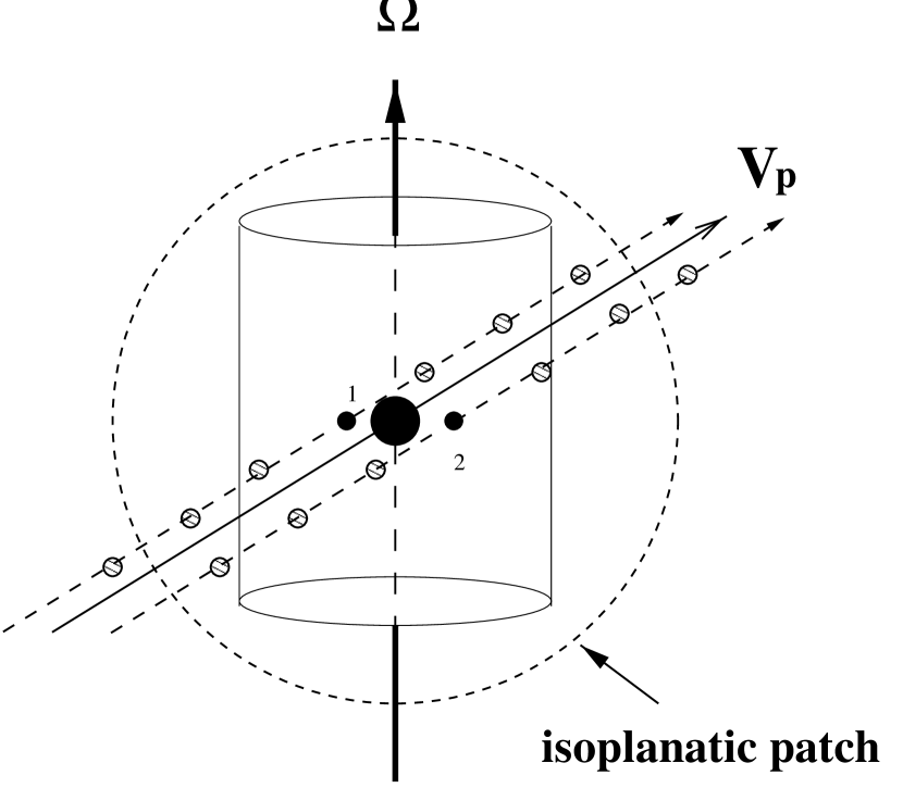
Figure 5: Depiction of pulsar geometry and the isoplanatic patch size for DISS. The cylinder indicates a portion of the velocity of light cylinder, the spin axis $\Omega$, and the pulsar’s transverse space velocity $V_{p}$. The large filled circle on the spin axis represents the neutron star while the smaller dots labelled 1 and 2 represent two emission regions that correspond, e.g., to two separate pulse components. The spatial offset between the emission regions in principle can be measured by investigating the differential dynamic spectrum between the two pulse components. The circles along the dashed tracks indicate the spatial locations of the emission regions as the pulsar moves in the plane of the sky. The size of the isoplanatic patch is a strong function of the scattering strength, being smaller for larger scattering. Thus using DISS to resolve particular objects requires flexibility in the choice of frequency. Adequate time and frequency resolutions are also required to sample the DISS appropriately.

2.3 Intraday Variability: RISS Superresolution

Intraday variability (IDV) refers to the hourly to daily intensity fluctuations exhibited by approximately 15% of all compact, flat-spectrum extragalactic sources at centimeter wavelengths [44]. The phenomenon was first identified as “flickering” on time scales of less than two days [27], and variations on timescales of less than twelve hours were reported soon after [75]. It was unclear whether the variations were intrinsic to the sources themselves or a result of propagation effects in the ISM. Initial tentative evidence in support of the former [53] was particularly concerning because it implied source brightness temperatures in excess of $10^{19}$ K, well above the inverse Compton limit. The problem was exacerbated by the discovery of 40–60 min. variations in PKS 0405$-$385 [37] for which the variations, if intrinsic, would imply a brightness temperature $10^{21}$ K.

It is now clear that the varations are not solely intrinsic to the sources themselves but are due at least partially, if not fully, to ISS. The case for ISS hinges on two distinct observational properties of IDV sources. The first is the measurement of significant time delays between widely separated telescopes in the variability patterns of the three fastest IDV sources, PKS 0405$-$385 [37], J1819$+$3845 [22], and PKS 1257$-$326 [3]. The delay arises because the intensity fluctuations caused by the scattering medium move across the line of sight with a finite speed (which is a vector sum between the Earth and medium’s velocities), so that there is a finite delay between the intensity fluctuations observed on $\sim 5000$ km baselines. The effectiveness of this technique depends on the ability to measure significant flux density changes on timescales shorter than the time delay between the two telescopes, typically 30–600 s. Time delay experiments have so far been limited to only the three strong sources whose variations are sufficiently strong and rapid.

The second is that annual cycles in the variability timescales of the fluctuations are observed in a number of IDV sources. This cycle arises because the speed of the scattering medium responsible for the ISS is comparable to Earth’s orbital speed around the Sun. The scintillation fluctuations are slowest when the Earth moves parallel to the scattering medium and are fastest when Earth moves antiparallel to the medium. Annual cycles have now been found for five sources, including J1819$+$3845 [20], B0917$+$624 [58, 33], and PKS 1257$-$326 [3], and there is increasing evidence (e.g., from the MASIV survey [44]) that it is present in a number of other sources exhibiting centimeter-wavelength IDV. This technique has established ISS as the principal mechanism responsible for IDV for sources whose variations are too slow ($>2$ hr) to be amenable to time delay experiments.

The variations in IDV sources generally exhibit the largest fractional modulations at frequencies $\nu\approx 5\,$GHz. Faster, less highly modulated variations are observed at higher frequencies, while the variations at lower frequencies are much slower with considerably lower amplitude. The change in the character of the scintillations is interpreted in terms of a transition between weak and strong ISS, with the slow variations at lower frequencies being due to RISS and the faster variations at higher frequencies being due to WISS.

The small diameters required to exhibit ISS imply uncomfortably high brightness temperatures for IDV sources. A source must be no more than tens of microarcseconds in diameter to display IDV at 5 GHz for a scattering screen at a distance of order 100 pc (§2.1). Brightness temperatures of order $5\times 10^{12}$ K have been determined for B1257$-$326 and J1819$+$3845 while the lower limit for B1519$-$273 is $5\times 10^{13}$ K and it could be as high as $6\times 10^{14}$ K [46]. While these brightness temperatures are lower than early estimates, in which the variations were interpreted as being solely intrinsic, they are still well above the inverse Compton limit. Doppler beaming can reduce these estimates further, but the required Doppler factors are as high as several hundred [54], significantly higher than seen in existing VLBI surveys [78, 73, 36].

Further information about source structure can be obtained by utilizing polarization. Even a rudimentary analysis shows that the linearly polarized structure of J1819$+$3845 at 5 GHz consists of at least two separate sources, separated by roughly 50 $\mu$as and indicates their location relative to the rest of the unpolarized emission. Analysis of the total intensity and circular polarization fluctuations in PKS 1519$-$273 indicates that this source consists of a 15–35 $\mu$as core with an extremely high circular polarization of $-3.8\pm 0.4$% [46]. Continuing observations of this source indicate the intermittent generation of circular polarization of opposite handedness in the core, suggesting that the source undergoes small, otherwise undetectable, outbursts every few months.

The sensitivity of the SKA is such that it potentially will probe the nanoarcsecond scale of extragalactic sources. It should be capable of detecting scintillating sources as much as three orders of magnitude fainter than those detected currently. Assuming that these fainter sources have incoherent synchrotron components in them, the implied angular scales are at least one and possibly two orders of magnitude smaller, so on the 1 $\mu$as to 100 nas scales. One microarcsecond corresponds to about 1 light-week at cosmological distances, and it is on these scales that jets are expected to be “launched.”

If there are such compact sources, the scintillation timescales would be even faster and modulation indices potentially higher; DISS might even be detected. Observations of time delays between Stokes parameters will yield differential source structure, and monitoring these delays will lead to the evolution of these components.

2.4 Strong Refractive Events

A small number of pulsars have displayed “strong fringing events” in their dynamic spectra, in which the normal, random appearance of the dynamic spectrum is modified by the appearance of quasi-periodic fringes (Figure 3). These fringes are interpreted most naturally as the beating of two distinct images of the pulsar. Multiple imaging of a pulsar can occur if there is a temporary increase in the power on refractive scales ($\sim 10^{13}$ cm) along the line of sight, e.g., as due to a discrete “cloud” of electrons drifting in front of the pulsar [18, 7].

The fringe spacing in the dynamic spectrum can be related to the angular separation of the multiple images formed by the strong refraction. The typical angular separation in the observed cases is a few milliarcseconds [18, 76]. Moreover, in order for fringes to occur, the multiple images must be at least partially coherent. Consequently, the strong refraction forms an interferometer with an effective baseline of 1 AU, and angular resolution of 1 $\mu$as. In the cases observed, the fringes displayed a dependence on pulse phase, which in turn indicated that the size of the emitting region must be of order $10^{8}$ cm.

The duty cycle of strong fringing effects, though not known with precision, is small; it is not clear if the discrete density structures occur along a few, specific lines of sight or if the discrete density structures are ubiquitous but have a small filling factor.

Multiple imaging is also expected from AGN undergoing “extreme scattering events” (ESE) [24, 62, 7]. Because of their intrinsically larger diameters, DISS does not occur and dynamic spectra are not determined. Imaging of a source undergoing an ESE may show the multiple imaging, if the image separation is larger than the scattering diameter. Unfortunately, the only VLBI observations of a source undergoing an ESE do not included the egress of the source from the ESE, when the image separation is predicted to be the largest [40].

3 The Microphysics of the Interstellar Plasma

For observations at 1 m wavelength over a length scale of 1 kpc, the Fresnel scale is $R_{F}\sim 10^{10}\,\mathrm{cm}\sim 10^{-8}\,\mathrm{pc}$. Scattering provides a powerful probe of interstellar physics from parsec scales down to a a few hundred kilometers.

Our heuristic descriptions of scattering observables and scintillation regimes can be cast more rigorously in terms of moments of the electric field. Angular broadening is measured from the visibility function, a second moment of the field, while scintillation observables are measured from intensity correlation functions, fourth moments of the field. In general, analytical solutions cannot be obtained for all desired moments of the field in all scattering regimes, but the various moments can be shown to be related to moments of the radio wave phase, and as such, can be related to the phase and density fluctuation power spectra (e.g., [59]).

A useful parameterization of the spatial power spectrum of the interstellar density fluctuations (like those in the interplanetary medium) is a power law,

$$P_{\delta n_{e}}=C_{n}^{2}(z)\,q^{-\alpha}e^{(ql_{1})^{2}/2}.$$ (7)

Here $q$ is the spatial wavenumber; $l_{1}$ is the inner scale or smallest length scale on which fluctuations are maintained; and $C_{n}^{2}(z)$, which is slowly varying with distance ($z$), describes the strength of the fluctuations along the line of sight, and is proportional to the rms density. Although not incorporated explicitly into equation (7), there is presumably also an outer scale $l_{0}$ describing the largest length scales on which density fluctuations are maintained.

A variety of studies have found that, in the solar neighborhood, $C_{n}^{2}\sim 10^{-3.5}$ m^-20/3, $\alpha\approx 3.7$, $l_{1}\mathbin{\lower 3.0pt\hbox{$\hbox to0.0pt{\raise 5.0pt\hbox{$\char 60\relax$}\hss}\mathchar 29208\relax$}}10^{9}$ cm ($\sim 10^{-9}$ pc), and $l_{0}\mathbin{\lower 3.0pt\hbox{$\hbox to0.0pt{\raise 5.0pt\hbox{$\char 62\relax$}\hss}\mathchar 29208\relax$}}10^{14}$–$10^{18}$ cm ($\sim 10^{-4}$–1 pc) [1]. Figure 6 presents a unified picture of the density fluctuations in the interstellar plasma. The power spectrum of the fluctuations (either density or magnetic field fluctuations) is plotted as a function of wavenumber along with representative data. Also indicated are the wavenumber regimes sampled by the different techniques described in this chapter. We now consider various aspects and implications of this parameterization for the spatial power spectrum.

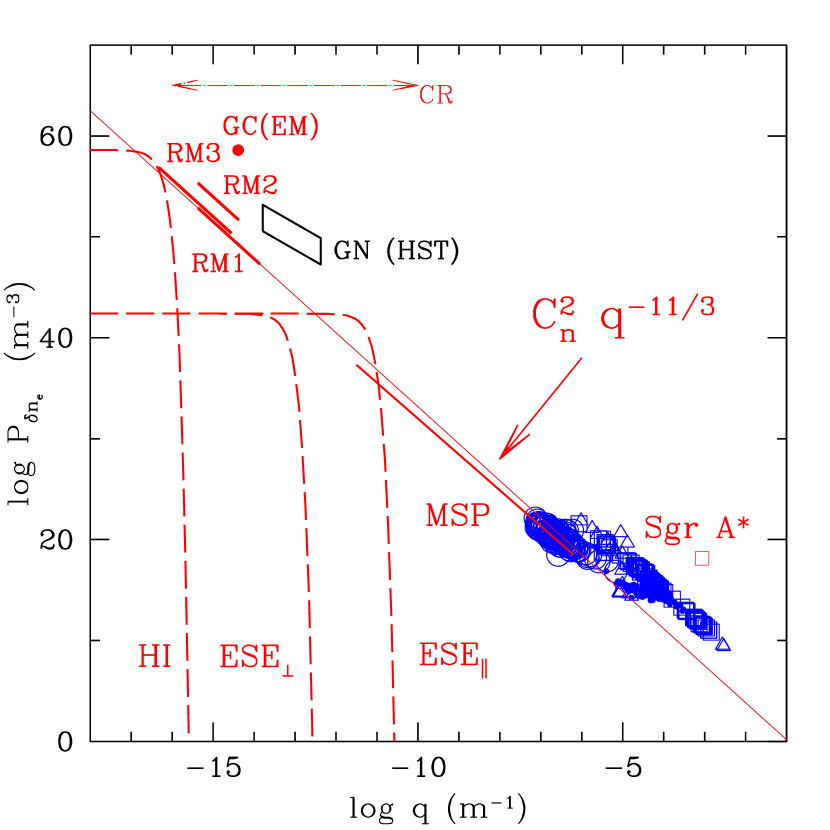
Figure 6: The spatial power spectrum of interstellar electron density fluctuations as probed by various methods. At high spatial frequencies ($\sim 10^{-5}$ m^-1) there are various diffractive measurements derived from pulsar scintillation measurements and angular broadening measurements, largely of extragalactic sources. The box centered roughly on $10^{-10}$ m^-1 illustrates limits placed from millisecond pulsar (MSP) timing measurements [17]. The boxes labelled “RM1,” “RM2,” and “RM3” result from various RM studies [65, 41, 49]. The box labelled “GN (HST)” results from Hubble Space Telescope observations of the Guitar Nebula. The arrows at the top indicate the approximate range of spatial scales for magnetic field fluctuations in order for cosmic ray protons (CR) to be sufficiently scattered.

3.1 Magnetohydrodynamic Turbulence and Interstellar Scattering

It is easy to show that the interstellar plasma has a large Reynolds number. Moreover, the density spectral index $\alpha\approx 11/3$, close to the value expected for Kolmogorov turbulence. This combination, the value for $\alpha$ and the plasma Reynolds number, suggests that the interstellar density fluctuations are the result of a turbulent process.

There are a number of significant caveats to this conclusion. Kolmogorov turbulence theory was developed initially for a neutral, incompressible medium—assumptions that the ISM clearly violates. If interstellar scattering is an observational manifestion of turbulence, the implied inertial range (between $l_{1}$ and $l_{0}$) is at least 5 orders of magnitude and potentially as much as 10 orders of magnitude, and it is not clear how to sustain such a large inertial range. Moreover, strong refractive events (§2.4) likely indicate the presence of discrete density structures.

Much progress, on both the observational and theoretical fronts, has been made in the past decade in explaining the density fluctuations responsible for interstellar scattering in terms of turbulence. From the theoretical perspective, the (mean) magnetic field energy density in the interstellar plasma is comparable to or much greater the gas kinetic energy density or thermal pressure. Thus, a theory for turbulence in magnetohydrodynamics (MHD) must be used. On the one hand, an MHD approach seems attractive as, for instance, density fluctuations are a natural result of Alfvén waves. On the other hand, it is probable that, at least on some spatial scales, the nonlinear terms in the MHD equations are important and a perturbative approach is not valid. Over the past decade, there has been a renewed interest in understanding MHD turbulence as it applies to interstellar density fluctuations [68, 26, 25, 50, 43, 42]. A key aspect of a turbulent description, though, is that on the smallest spatial scales the kinetic energy of the turbulence is dissipated and heats the medium. Cooling mechanisms within the medium must be capable of radiating this heat lest a “thermodynamic catastrophe” result [66]. Estimates of the dissipation heating from various damping mechanisms can be used to constrain the nature of the turbulence [48].

On the observational front, there has also been considerable progess in establishing that there are magnetic field fluctuations accompanying (or more likely driving) the density fluctuations responsible for scattering. RM and EM structure function analyses across several degrees of sky show the structure functions to have power-law spectra, at least on scales less than roughly 1 pc, consistent with what is expected from a turbulent process [49, 30]. Importantly, the RM structure function analyses require both magnetic field and density fluctuations, as expected if the density fluctuations result from magnetic field fluctuations in a turbulent magnetized fluid.

3.2 Anisotropy

In MHD turbulence, it is expected that density fluctuations would be aligned along the field direction and potentially be highly anisotropic. If the density fluctuations are elongated, scattering observables would be affected, e.g., scattering disks of sources would be anisotropic. Such an effect is seen in the solar wind.

A small number of highly scattered sources do display anisotropic scattering disks, with typical aspect ratios of a few. The aspect ratios are much smaller than what is expected for the density fluctuations (for which aspect ratios of tens to hundreds may be obtained). However, if these aspect ratios do result from elongated density fluctuations, the orientation of the magnetic field (and therefore of the density fluctuations) probably varies randomly along the line of sight with a typical correlation length comparable to the outer scale. If the path length through the scattering medium is much longer than the outer scale, averaging would reduce the observed aspect ratio well below the intrinsic aspect ratio of the density fluctuations.

More recently, IDV observations suggest that density fluctuations in the more general ionized interstellar medium (as opposed to particularly heavily scattered lines of sight) may also be anisotropic. An axial ratio $\sim 4$:1 is derived for PKS 0405$-$385 [57] and $15:1$ for J1819$+$3845 [20]. In the latter case, this aspect ratio probably reflects not only scattering but intrinsic structure within the source (i.e., jet structure). Nonetheless, the anistropy intrinsic to the scattering medium is still at least 4:1 in this source.

Indeed, for two sources, Cyg X-3 and NGC 6334B, the orientations of the scattering disks change as a function of $\lambda$ [74, 72]. Both groups identify the orientation changes as due to the magnetic field aligning density fluctuations on different length scales. Notably, though, neither Sgr A^∗ (e.g., [61, 77]) nor the extragalactic source B1849$+$005 [39] show any orientation changes with wavelength, even though the angular broadening for both has been measured over a larger range in wavelength than for either Cyg X-3 or NGC 6334B.

3.3 Inner Scale

In a turbulent process the inner scale $l_{1}$ is the scale on which turbulent energy is dissipated and heats the medium. Estimates of the turbulent heating rate of the medium and avoidance of a thermodynamic catastrophe rely on obtaining a robust estimate of its value.

Comparing various VLBI observations, Spangler & Gwinn [67] found evidence for an apparent change in the slope of the density spectrum (i.e., change in $\alpha$) on baselines $b\sim 200$ km, consistent with detecting an inner scale of approximately this magnitude. They attribute the inner scale to either the ion inertial length or Larmor radius.

3.4 Cosmic Ray Propagation and MHD Turbulence

Galactic cosmic rays are observed to have an isotropic arrival direction and have an energy spectrum that is a continuous power law over the approximate energy range of 1 to $10^{6}$ GeV per nucleon. (The power law may extend to lower energies, but solar modulation becomes increasingly important at lower energies.) Jokipii [35, 34] has argued that these characteristics of cosmic rays require a wide-band spectrum of magnetic field fluctuations.

The absence of any “breaks” or “bumps” in the spectrum as well as an isotropic arrival direction indicate that a typical cosmic ray undergoes many scatterings during its lifetime. Cosmic rays are scattered most effectively by magnetic field fluctuations on length scales near their gyroradii. In this energy range, the relevant gyroradii are $10^{12}$–$10^{18}$ cm, suggesting that the spectrum of magnetic field fluctuations encompasses at least this range of length scales. As described above, there is modest evidence from RM structure function analyses for magnetic field fluctuations at the upper end of these length scales, while refractive effects and DM monitoring programs can probe density fluctuations at the lower end of these length scales.

The large number of scatterings that cosmic rays experience also makes them of limited utility in studying the magnetic field fluctuations, other than indicating that magnetic field fluctuations may exist. The diffuse Galactic gamma-ray emission at energies $E>100$ MeV results from the interaction of cosmic rays with the interstellar matter and radiation fields [4, 23] and suffers essentially no absorption or scattering over Galactic distances. As such it is a powerful diagnostic of the Galactic distribution and propagation of cosmic rays.

Typical models for the diffuse $\gamma$-ray emission utilize expressions like equation (6) in which $n_{n}$ is approximated by the hydrogen distribution $n_{H}$ and $q_{\gamma}$ is taken to be constant or slowly varying. These models have proven quite successful in reproducing the large-scale features—an enhancement in the inner Galaxy and spiral-arm tangents—seen in maps of $I_{\gamma}$ (e.g., [70, 2, 32]). In such models, variations in $I_{\gamma}$ arise essentially from variations in $n_{H}$. However, there are departures of the data from the model. In some famous cases, these are due to discrete sources (Geminga, Crab pulsar, Vela pulsar) while in others, they are essentially unidentified “hot spots” in the gamma-rays.

“Hot spots” and other variations in $I_{\gamma}$ might also result from fluctuations in $q_{\gamma}$. In particular, magnetic fluctuations can act not only to scatter cosmic rays, but also to confine them [47]. Therefore, enhancements in $I_{\gamma}$ could result either from an increase in the ambient matter density or from a longer cosmic-ray residence time in regions of enhanced magnetic turbulence or both. If the density fluctuations responsible for interstellar scattering result from the same magnetic fluctuations responsible for cosmic-ray confinement, as appears likely on at least the largest scales, radio-wave scattering data can be used to predict $q_{\gamma}$. Conversely, gamma-ray observations could provide an additional indirect probe of magnetic field fluctuations on length scales smaller than those probed by Faraday rotation variations and complementary to those probed by radio-wave scattering observations and the energy spectrum of Galactic cosmic rays (Figure 6).

To date, little has been done to test these ideas, due at least in part to the fairly coarse angular resolution of $\gamma$-ray telescopes. In comparison to the sub-arcsecond resolution of the radio telescopes typically used to study interstellar scattering, past $\gamma$-ray telescopes have had angular resolutions of a few degrees or worse. More problematic, these angular resolutions also have been fairly coarse when compared with the diameter of a typical scattering region over Galactic distances. For instance, a region 1 pc in diameter at a distance of 8 kpc (comparable to the mean free path between intense scattering regions [16]) subtends an angle of only $0.5^{\prime}$. The effects we describe may nonetheless be detectable with future $\gamma$-ray instruments with higher angular resolutions operating during the SKA’s lifetime.

Not only could comparisons of radio and $\gamma$-ray observations yield information about the magnetic field on sub-parsec scales, but radio observations could be used to improve models for the Galactic distribution of the diffuse $\gamma$-ray emission.

The diffuse Galactic $\gamma$-ray emission can (probably does!) obscure faint point and small-diameter sources (neutron stars, black holes, $\gamma$-ray blazars, young supernova remnants, or even an as-yet unidentified class of $\gamma$-ray emitters). For example, there are presumably more Geminga-like $\gamma$-ray pulsars in the Galaxy. Separating more distant and/or intrinsically weaker $\gamma$-ray point sources from the diffuse emission requires better understanding of the diffuse emission, particularly on smaller angular scales. Indeed, the detection of Geminga itself may have been somewhat fortuitous in that it was both nearby and toward the galactic anticenter, where the diffuse emission is less intense.

4 Distance Determinations from Interstellar Scattering

The conventional factorization of the density spectrum allows for different lines of sight to have similar microphysics (wavenumber scaling) but differing scattering strengths (coefficient $C_{n}^{2}$). Values for SM, the line-of-sight integral of $C_{n}^{2}$, can be estimated from angular broadening measurements of extragalactic sources or Galactic sources (typically pulsars or masers), pulse broadening measurements for pulsars, or scintillation bandwidth measurements for pulsars. In general, only angular broadening measurements of extragalactic sources yield SM directly. For the other kinds of measurements, a line-of-sight weighting of the scattering material must be taken into account in order to extract SM; for angular broadening of Galactic sources, scattering material close to the observer is most strongly weighted while for pulse broadening and scintillation bandwidth scattering material mid-way between the pulsar and observer is most strongly weighted.

Comparisons of SM along different lines of sight yield the angular distribution of density fluctuations, which can be inverted to obtain a spatial distribution, while comparisons of SM on similar lines of sight (e.g., pulsar vs. AGN) constrain the radial distribution of density fluctuations. For pulsars, in principle, one also can compare the magnitude of angular broadening to the pulse broadening or scintillation bandwidth to obtain the line-of-sight weighting directly.

4.1 The Galactic Distribution of the Interstellar Plasma

Although measurements of only SM can be used to obtain the angular distribution of density fluctuations, they are much more powerful when combined with measurements of pulsar DMs, and pulsar parallaxes to produce three-dimensional models for the Galactic distribution of the interstellar plasma. The most recent effort is the NE2001 model (so named because it is based on data obtained up to 2001, [13, 14], Figure 7), which uses roughly 1200 pulsar DMs, 300 measurements of SM, and 100 measurements of DM-independent pulsar distances (e.g., parallaxes or pulsar-supernova remnant associations). Not only does this model describe the Galactic distribution of the interstellar plasma, it can be used to predict the distances of pulsars from their DMs.

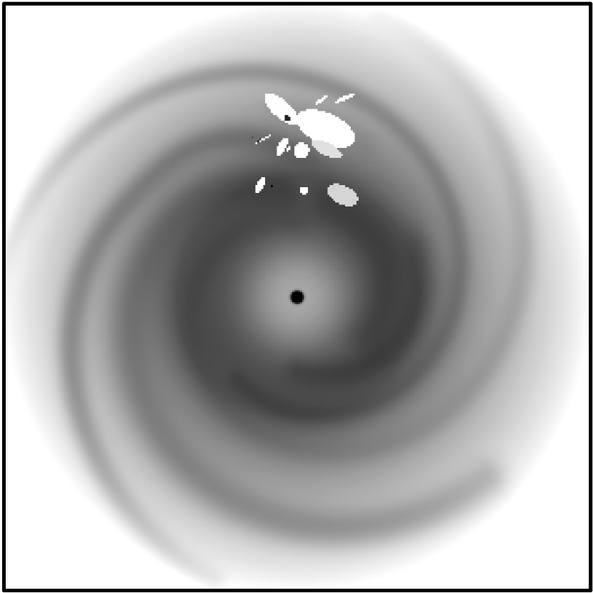
Figure 7: The Galactic distribution of the free electron density, as described by the NE2001 model. Shown is a face-on view of the Galaxy with the Galactic center at the center. Three large-scale components of the model—the inner Galaxy component centered on the molecular ring, the spiral arms, and the diffuse component—are all clearly visible. Also visible are a number of “voids,” such as the Local Bubble, some of the mesoscale structures required in the model in order to reproduce various pulsar or scattering observables. The Sun is near the black dot in the center of the Local Bubble in the upper portion of the figure.

The NE2001 model (like many of its predecessors) describes the Galaxy in terms of large-scale components—a thin disk, a thick disk, and spiral arms. Although less true than in some previous models, the SM and DM measurements still play a largely complementary role in the NE2001 model. Most pulsars are relatively faint so their DMs probe the interstellar plasma only relatively nearby ($\sim 1$ kpc); most measurements of SM are toward extragalactic sources so the lines of sight are relatively long ($\sim 10$ kpc). The combination of the DM and SM values thus allows for the possibility of a global model. With the increasing number of distant pulsars and their DMs, particularly from the Parkes multi-beam survey, the NE2001 model is perhaps more equitable in the balance between DM and SM for long lines of sight, though the SM values remain important.

A novel feature of the NE2001 model is the systematic introduction of “clumps” and “voids,” regions of enhanced or decreased electron density and/or scattering. Previous models had contained a localized enhancement (clump) due to the Gum Nebula because it is so close to the Sun, but the current number of measurements of DM and SM is becoming sufficient that not only large-scale features (e.g., diffuse ionized disk, spiral arms) can be modeled but also mesoscale structures (e.g., H ii regions). On a limited number of lines of sight, reasonable agreement between a modeled and observed quantity (DM and/or SM) could be obtained only by inserting either a clump or a void.

The SKA will provide qualitatively new means of constructing global models. One of the Key Science Projects for the SKA is a pulsar census of the Galaxy (Kramer et al., this volume; Cordes et al., this volume), which will necessarily include the DMs for all of the pulsars found. It is expected that such a census will increase the number of pulsars by a substantial factor ($\sim 5$). We expect that the number of pulsar parallaxes will also increase by a similar amount. The number of pulsars will be sufficiently large that there should be several per degree along the Galactic plane. Consequently, the lines of sight to distant pulsars will have a reasonable probability of intersecting an H ii region even over Galactic distances ($\sim 10$ kpc).

The density of pulsars on the sky will decrease with increasing Galactic latitude of course, but these can be supplemented with scattering measurements and IDV observations. Assuming that the density of IDV sources on the sky is sufficiently high, the characteristic frequency at which IDV is strongest can be determined as a function of Galactic latitude, in a manner analogous to observations of interplanetary scintillation at lower frequencies (e.g., [55]).

We suggest that the number of measurements provided by the SKA will be sufficiently large that it will be possible to trace the Galaxy’s structure, or at least its spiral structure, in a self-consistent manner, rather than by imposing it as has been done for the NE2001 and previous models. The methodology would be to insert clumps of increased electron density, representing H ii regions, along the line of sight to pulsars and extragalactic sources. The clumps would be inserted in a parsimonious manner so as to minimize the difference between observed and predicted DMs and SMs with the minimum number of clumps. As spiral arms are not smooth structures, voids may also need to be inserted in a similar manner. Moreover, combining scattering measurements, e.g., pulsar pulse broadening and angular broadening, would constrain the radial distribution of scattering (e.g., [6]).

A second Key Science Project (see chapter by Gaensler, this volume), is the production of a grid of extragalactic sources with measured RMs. Although not used to date in constructing models for the Galactic distribution of the interstellar plasma, such a grid offers exciting possibilities for expanding the NE2001 model (or its successors) to describe the magnetoionic medium in terms of both $n_{e}$ and $B$.

4.2 Local Interstellar Medium

IDV sources are excellent probes of the scattering material within roughly 10–50 pc of the Sun. The prominence of such local scattering material in IDV scattering would, at first sight, appear to be surprising, since pulsar radiation tends to be scattered at greater distances. However, for WISS and RISS, the finite angular diameters of IDV sources produce a weighting with nearby scattering material being most important. This effect arises because WISS and RISS tend to be dominated by scattering material whose distances are such that the angular diameter of the first Fresnel zone closely matches the source angular diameter [8, 9]. The combination of a large number of IDV measurements along with pulsar scattering measurements and parallaxes should yield similar qualitative advances in the description of the local ISM.

5 Intergalactic Scattering

Radio-wave scattering is a generic process that occurs whenever radio waves pass through a medium containing density fluctuations. To date, observable effects have been seen from the Earth’s ionosphere (e.g., ionospheric scintillations), the interplanetary medium (e.g., interplanetary scintillations and spectral broadening), and the interstellar medium (see above). That a small number AGN display intraday variability and a small number of gamma-ray burst afterglows display interstellar scintillation indicates that at least some lines of sight through IGM are not scattered appreciably. If these lines of sight were scattered, these sources would be too heavily broadened to display interstellar scintillation.

Nonetheless, the IGM would appear to have the characteristics necessary for intergalactic scattering to be obtained. For redshifts $z\mathbin{\lower 3.0pt\hbox{$\hbox to0.0pt{\raise 5.0pt\hbox{$\char 60\relax$}\hss}\mathchar 29208\relax$}}6$, the absence of a Gunn-Peterson trough in quasar spectra indicates that the IGM is largely ionized, and recent far-ultraviolet and soft X-ray observations of highly ionized species (e.g., O vi) along the line of sight to various low-redshift quasars may be a direct detection of the ionized IGM [51, 71, 56, 64, 63]. In the prevailing “cosmic web” scenario for large-scale structure formation, most of the baryons are in filamentary structures which are themselves permeated by shocks. Thus, it is expected that the IGM is both ionized and “turbulent.” Moreover the long path lengths through the IGM ($>100$ Mpc) as compared to the ISM ($\sim 1$–10 kpc) may compensate for the lower density ($\sim 10^{-7}$ cm^-3 vs. 0.025 cm^-3, respectively).

Detection of intergalactic scattering would be a powerful probe of the IGM, as it would be caused by the majority of the baryons. Observations of the Ly$\alpha$ forest probe mostly the neutral component, which represents only about $10^{-5}$ of the mass. The metallicity of the IGM is highly uncertain, so the ionized gas traced by the far-ultraviolet and soft X-ray observations represents a small and uncertain fraction of the total mass.

Cordes & Lazio [12] have considered intergalactic scattering from the general IGM, expanding on previous treatments of scattering from intra-cluster media [29]. In analogy to interstellar scattering, dispersion and scattering measures from the IGM can be defined and both diffractive and refractive scattering effects can be described. We summarize their conclusions briefly.

The expected DM through the IGM is $\mathrm{DM}\mathbin{\lower 3.0pt\hbox{$\hbox to0.0pt{\raise 5.0pt\hbox{$\char 62\relax$}\hss}\mathchar 29208\relax$}}1000$ pc cm^-3 for sources with redshifts $z\mathbin{\lower 3.0pt\hbox{$\hbox to0.0pt{\raise 5.0pt\hbox{$\char 62\relax$}\hss}\mathchar 29208\relax$}}4$. A similar estimate has been found by Palmer [52]. This value is comparable to path lengths of order a few kiloparsecs through the ISM.

The expected SM through the IGM depends upon location of the bulk of the scattering material. If the bulk of the scattering arises in galaxies like the Milky Way (rather than the diffuse IGM), $\mathrm{SM}\sim 10^{-4.5}$ kpc m^-20/3. Estimating the scattering measure in the diffuse IGM requires assumptions about the distribution and power spectrum of density fluctuations in the IGM. Assuming that the density fluctuations are in “cloudlets,” (as in the ISM), they estimate that scattering measures as large as $\mathrm{SM}\sim 10^{-3}$ kpc m^-20/3 may be obtained. In the latter case, scatter broadening diameters of order 1 mas are implied. As in the interstellar case, there is a geometrical weighting factor for the distribution of density fluctuations along the line of sight, with material closest to the observer having the largest weight. For intergalactic scattering, there is an additional wavelength-dependent weighting, that also favors scattering material close to the observer; at higher redshifts, the wavelength of the propagating radiation is shorter and scattering is generally less effective.

Figure 8 shows predictions for the amount of angular broadening expected at selected frequencies, based on a model in which the bulk of the IGM is the form of electron density “cloudlets.” At 1.4 GHz an angular resolution better than 4 mas is required to detect intergalactic scattering. Such an angular resolution is at the limit of what can be achieved with terrestrial baselines. Reliable detection of intergalactic scattering at 1.4 GHz probably will require space-based VLBI, though the SKA will prove valuable in increasing the senstivity of such future VLBI arrays.

At 0.33 GHz an angular resolution better than 80 mas is required. This requirement is easily within the capabilities of existing VLBI networks. For instance the highest angular resolution of the VLBA at this frequency is 25 mas. The key difficulty with existing VLBI arrays is their relative lack of sensitivity at this frequency. Even if only a small fraction (5–10%) of the SKA is distributed on continental/intercontinental baselines, its sensitivity could exceed existing VLBI arrays at this frequency by as much as a factor of $10^{3}$. Such a large increase in sensitivity would produce a significant increase in the number of sources that could be searched for scattering from the IGM and enable robust statistical analyses, e.g., for trends with redshift.

At 0.15 GHz the required angular resolution to detect intergalactic scattering is 500 mas, equivalent to baselines of order 1000 km. It is not yet clear if the SKA will operate at 0.05 GHz, but, if it should, an angular resolution better than 5^′′, equivalent to baselines of 250 km, is required. It is not clear that sufficiently compact objects exist at cosmological distances to be detected at 0.05 GHz, though, at a redshift of 5, for example, the rest frame emission would occur at 0.3 GHz. At both frequencies, the required baselines are well within the nominal goals for the SKA.

Thus, detection of possible intergalactic scattering requires the SKA to have intercontinental baselines at 0.33 GHz or baselines of order 1000 km below 0.2 GHz or both.

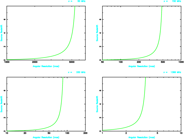
Figure 8: Source redshift required to produce angular broadening of a given magnitude at four typical observation frequencies. Clockwise from upper left, the four frequencies are 0.05, 0.15, 0.33, and 1.4 GHz. The curves shown assume that the scattering medium is intergalactic clouds with $\Omega_{\mathrm{H\,II}}\sim 0.04$.

6 The Variable (Scintillating) Sky and SKA Synthesis Observations

At the sensitivity levels reached by the SKA, we may expect to see many scintillating radio sources within the field of view. It is been often stated, and generally believed, that variability will severely limit the dynamic range of synthesis images. We consider two extreme cases to illustrate why this is not necessarily so.

The most frequently encountered case will be that the total average flux density of all scintillating sources in the field of view during the observation is small fraction of the total flux density contributed by all sources. Consequently, the scintillating sources cannot have a large effect on the self-calibration solution.

In the other extreme case, the average flux density of the scintillating source dominates the total flux density in the field of view. After the light curve of the scintillating source has been determined, it can be subtracted from the visibility data in a time-dependent manner. Standard imaging and self-calibration can be applied to the residual visibility data.

7 Why the SKA and What is Needed?

An important aspect of many of kinds of observations relevant to superresolution imaging and turbulent phenomena is that they represent a class of non-imaging analyses that the SKA should be capable of performing. In general, these observations require that some (large) fraction of the SKA’s collecting area be capable of being operated in a phased-array mode, in which the voltages from the individual collectors are delayed appropriately and then summed.

Exploiting the SKA to study the structure of both extragalactic sources and pulsars as well as of the magnetoionic Galactic interstellar medium requires that a variety of observables be measurable. In many cases these observables are similar to what is needed to exploit observations of transient radio sources (Cordes et al., this volume) and GRB afterglows (Weiler, this volume), and, as pulsars form an important target, similar to the requirements for exploiting observations of pulsars (Cordes et al., this volume; Kramer et al., this volume).

Dynamic spectra

Probing source structure with superresolution as well as the scattering properties of the ISM requires multiepoch dynamic spectra (Figure 3). In general for probing source structure, the key promise of the SKA is its sensitivity. Many of the relevant observations can be conducted at the present time or in the near future, but only on a small number of sources, so it is not clear to what extent these sources represent typical or representative examples. The utility of dynamic spectra for a source is that, if there is sufficient sensitivity to form dynamic spectra as a function of time, modifications in the DISS characteristics in the differential dynamic spectra indicate the presence of structure on sub-$\mu$as angular scales. For some applications, the dynamic spectra should be obtained for all Stokes parameters.

For pulsars, dynamic spectra formed a function of pulse phase can be used to assess the presence of multiple emitting regions within the pulsar magnetosphere (Figure 5). For GRB afterglows, a similar analysis could be used to detect and monitor the formation and evolution of components within the emitting shock regions. For AGN, if they do display DISS, the relevant scales probed are comparable to those on which jet formation is thought to occur near the central engine. For the case of AGN, dynamic spectra observations will complement those of future missions such as Constellation-X and GLAST, which will observe the highly-energetic emission from the bases of AGN jets.

Particularly for the case of pulsars, dynamic spectra also can be utilized to extract parameters such as the scintillation bandwidth, scintillation time scale, and scintillation velocity, and the arc phenomenon (Figure 4) seen in pulsar dynamic spectra can be used to constrain the electron density power spectrum. Although these parameters can be extracted from the current pulsar census with existing telescopes, the much larger pulsar census that the SKA will perform opens up the possibility of qualitatively new analyses in determining both the Galactic (§4.1) and line-of-sight (§4) distributions of scattering material.

These observations of dynamic spectra require time resolutions $\sim 1$ s and frequency resolutions $\sim 1$–100 kHz over wide bandwidths. In order to obtain dynamic spectra as a function of pulsar pulse phase, sampling times of 10 to 100 $\mu$s are needed.

Pulse broadening

Measurement of pulse broadening of pulsar pulses enables characterization of SM along heavily scattered lines of sight, complementing those for which dynamic spectra can be used, and constrains the wavenumber spectrum for $\delta n_{e}$ and the distribution along the line of sight of scattering material.

As with dynamic spectra, pulse broadening can be determined for a small number of pulsars with existing telescopes, but the SKA offers the promise of a greatly increased number of pulsars toward which pulse broadening can be determined. In particular, measurements of pulse broadening in the the much larger pulsar census provided by the SKA are important for the possibility of qualitatively new analyses in determining the Galactic distribution of the interstellar plasma (§4.1). “Clumps” in the interstellar plasma, as introduced in the NE2001 model, produce enhanced pulse broadening and so may enable the Galactic spiral arms to be traced, in part, by pulse broadening.

These observations require time resolutions, channelization, and post processing identical to that needed for pulsar timing (Cordes et al., this volume).

Angular broadening

Probing the Galactic (and intergalactic?) and line-of-sight distributions of scattering material as well as comparing radio-wave and $\gamma$-ray observations requires high angular resolution in order to measure angular broadening.

One of the strengths of angular broadening measurements toward AGN is that it provides a direct measure of the scattering strength along the line of sight. Other measures of scattering, e.g., pulse broadening, contain line-of-sight weightings for the scattering material. As for pulse broadening, angular broadening is a powerful probe of the Galactic plasma and, in terms of a qualitative improvement for the Galactic interstellar plasma (§4.1), a large census of SM values for AGN would complement the large pulsar census that the SKA will perform. Moreover, pulsars will not be detectable over cosmological distances, while AGN clearly are, so angular broadening offers the promise of a direct probe of the IGM (§5).

For angular broadening measurements, the most important aspect is transcontinental or intercontinental baselines. As described in §5, intercontinental baselines at 0.33 GHz or baselines of order 1000 km below 0.2 GHz or both are minimal requirements for angular broadening studies.

Light curves

In many current concepts, the SKA is envisioned as having a “core” and “outlying stations.” Not all observations will be able to make use of the entire SKA, e.g., use of the outlying stations produces too low of a surface brightness sensitivity for some kinds of H i observations. Thus, a small number of outlying stations could be used to form a sub-array and tasked to measure the flux density of a variety of objects, such as to monitor a large number of AGN for IDV or search for ESEs.

Table 1: Requirements for the SKA

Item	Requirement	Motivation
Time Resolution	10–100 $\mu$s	dynamic spectra
		pulse broadening
Frequency Resolution	1–100 kHz	dynamic spectra
Configuration	phased-array	pulsar observations
	operations possible
Configuration	sub-arrays possible	light curves
Configuration	$>1000$ km baselines	angular broadening

References

- [1] Armstrong, J. W., Rickett, B. J., & Spangler, S. R. 1995, ApJ, 443, 209
- [2] Bertsch, D. L., Dame, T. M., Fichtel, C. E., Hunter, S. D., Sreekumar, P., Stacy, J. G., & Thaddeus, P. 1993, ApJ, 416, 587
- [3] Bignall, H. E., et al. 2003, ApJ, 585, 653
- [4] Bloemen, H. 1989, ARA&A, 27, 469
- [5] Charnotskii, M. I., Myakinin, V. A., & Zavorotnyy, V. U. 1990, J. Opt. Soc. Am. A, 7, 1345
- [6] Claussen, M. J., Goss, W. M., Desai, K. M., & Brogan, C. L. 2002, ApJ, 580, 909
- [7] Clegg, A. W., Fey, A. L, & Lazio, T. J. W. 1998, ApJ, 496, 253
- [8] Codona, J. L. & Frehlich, R. G. 1987, Radio Science, 22, 469
- [9] Coles, W. A., Frehlich, R. G., Rickett, B. J., & Codona, J. L. 1987, ApJ, 315, 666
- [10] Cordes, J. M. 2004, ApJ, submitted; astro-ph/0007231
- [11] Cordes, J. M. 2004, ApJ, submitted; astro-ph/0007233
- [12] Cordes, J. M. & Lazio, T. J. W. 2004, ApJ, submitted
- [13] Cordes, J. M. & Lazio, T. J. W. 2002, astro-ph/0207156
- [14] Cordes, J. M. & Lazio, T. J. W. 2003, astro-ph/0301598
- [15] Cordes, J. M. & Lazio, T. J. W. 1991, ApJ, 376, 123
- [16] Cordes, J. M., Weisberg, J. M., Frail, D. A., Spangler, S. R., & Ryan, M. 1991, Nature, 354, 121
- [17] Cordes, J. M., Wolszczan, A., Dewey, R. J., Blaskiewicz, M., & Stinebring, D. R. 1990, ApJ, 349, 245
- [18] Cordes, J. M. & Wolszczan, A. 1986, ApJ, 307, L27
- [19] Cornwell, T. J. & Narayan, R. 1993, ApJ, 408, L69
- [20] Dennett-Thorpe, J. & de Bruyn, A. G. 2003, A&A, 404, 113
- [21] Dennett-Thorpe, J. & de Bruyn, A. G. 2002, Nature, 415, 57
- [22] Dennett-Thorpe, J. & de Bruyn, A. G. 2000, ApJ, 529, L65
- [23] Fichtel, C. E., et al. 1989, in Proc. Gamma Ray Observatory Science Workshop, ed. W. N. Johnson (NASA: GSFC) p. 3-1
- [24] Fiedler, R. L., Dennison, B., Johnston, K. J., & Hewish, A. 1987, Nature, 326, 675
- [25] Goldreich, P. & Sridhar, S. 1997, ApJ, 485, 680
- [26] Goldreich, P. & Sridhar, S. 1995, ApJ, 438, 763
- [27] Heeschen, D. S. 1984, AJ, 89, 1111
- [28] Haffner, L. M., Reynolds, R. J., Tufte, S. L., Madsen, G. J., Jaehnig, K. P., & Percival, J. W. 2003, ApJS, in press
- [29] Hall, A. N. & Sciama, D. W. 1979, ApJ, 228, L15
- [30] Haverkorn, M., Gaensler, B. M., McClure-Griffiths, N. M., Dickey, J. M., & Green, A. J. 2004, ApJ, in press
- [31] Harmon, J. K. & Coles, W. A. 1983, ApJ, 270, 748
- [32] Hunter, S. D., et al. 1997, ApJ, 481, 205
- [33] Jauncey, D. L. & Macquart, J.-P. 2001, A&A, 370, L9
- [34] Jokipii, R. 1999, in Interstellar Turbulence, eds. J. Franco & A. Carramiñana (Cambridge: Cambridge University Press) p. 70
- [35] Jokipii, J. R. 1988, in Radio Wave Scattering in the Interstellar Medium, eds. J. M. Cordes, B. J. Rickett, & D. C. Backer (New York: AIP) p. 48
- [36] Jorstad, S. G. & Marscher, A. P. 2003, in Radio Astronomy at the Fringe, eds. J. A. Zensus, M. H. Cohen, & E. Ros, (San Francisco: ASP) p. 89
- [37] Kedziora-Chudczer, L. et al. 1997, ApJ, 490, L9
- [38] Lazio, T. J. W., Cordes, J. M., & Fey, A. L. 2004, ApJ, in preparation
- [39] Lazio, T. J. W. 2004, ApJ, in press
- [40] Lazio, T. J. W., Fey, A. L., Dennison, B., et al. 2000, ApJ, 534, 706
- [41] Lazio, T. J., Spangler, S. R., & Cordes, J. M. 1990, ApJ, 363, 515
- [42] Lithwick, Y. & Goldreich, P. 2003, ApJ, 582, 1220
- [43] Lithwick, Y. & Goldreich, P. 2001, ApJ, 562, 279
- [44] Lovell, J. E. J., et al. 2003, AJ, 126, 1699
- [45] Macquart, J.-P. & Jauncey, D. L. 2002, ApJ, 572, 786
- [46] Macquart, J.-P., Kedziora-Chudczer, L., Rayner, D. P., & Jauncey, D. L. 2000, ApJ, 538, 623
- [47] McIvor, I. 1977, MNRAS, 179, 13
- [48] Minter, A. H. & Spangler, S. R. 1997, ApJ, 485, 182
- [49] Minter, A. H. & Spangler, S. R. 1996, ApJ, 458, 194
- [50] Ng, C. S. & Bhattacharjee, A. 1997, Phys. Plasmas, 4, 605
- [51] Oegerle, W. R., et al. 2000, ApJ, 538, L23
- [52] Palmer, D. M. 1993, ApJ, 417, L25
- [53] Quirrenbach, A., et al. 1991, ApJ, 372, L71
- [54] Readhead, A. C. S. 1994, ApJ, 426, 51
- [55] Readhead, A. C. S. & Duffett-Smith, P. J. 1975, A&A, 42, 151
- [56] Richter, P., Savage, B. D., Wakker, B. P., Sembach, K. R., Kalberla, P. M. W. 2001, ApJ, 549, 281
- [57] Rickett, B. J., Kedziora-Chudczer, L., & Jauncey, D. L. 2002, ApJ, 581, 103
- [58] Rickett, B. J., et al. 2001, ApJ, 550, L11
- [59] Rickett, B. J. 1990, ARA&A, 28, 561
- [60] Rickett, B. J. 1970, MNRAS, 150, 67
- [61] Rogers, A. E. E. et al. 1994, ApJ, 434, L59
- [62] Romani, R. W., Blandford, R. D., & Cordes, J. M. 1987, Nature, 328, 324
- [63] Savage, B. D., Sembach, K. R., Tripp, T. M., & Richter, P. 2002, ApJ, 564, 631
- [64] Sembach, K. R., Howk, J. C., Savage, B. D., Shull, J. M., & Oegerle, W. R. 2001, ApJ, 561, 573
- [65] Simonetti, J. H. & Cordes, J. M. 1986, ApJ, 310, 160
- [66] Spangler, S. R. 1991, ApJ, 376, 540
- [67] Spangler, S. R. & Gwinn, C. R. 1990, ApJ, 353, L29
- [68] Sridhar, S. & Goldreich, P. 1994, ApJ, 432, 612
- [69] Stinebring, D. R., McLaughlin, M. A., Cordes, J. M., Becker, K. M., Goodman, J. E. E., Kramer, M. A., Sheckard, J. L., & Smith, C. T. 2001, ApJ, 549, L97
- [70] Strong, A. W., et al. 1988, A&A, 207, 1
- [71] Tripp, T. M., Savage, B. D., & Jenkins, E. B. 2000, ApJ, 534, L1
- [72] Trotter, A. S., Moran, J. M., & Rodríguez, L. F. 1998, ApJ, 493, 666
- [73] Vermeulen, R. C., et al. 2003, in Radio Astronomy at the Fringe, eds. J. A. Zensus, M. H. Cohen, & E. Ros (San Francisco: ASP) p. 43
- [74] Wilkinson, P. N., Narayan, R., & Spencer, R. E. 1994, MNRAS, 269, 67
- [75] Witzel, A., Heeschen, D. S., Schalinski, C. J., & Krichbaum, T. P. 1986, Mitt. Astron. Ges., 65, 239
- [76] Wolszczan, A. & Cordes, J. M. 1987, ApJ, 320, L35
- [77] Yusef-Zadeh, F., Cotton, W., Wardle, M., Melia, F., & Roberts, D. A. 1994, ApJ, 434, L63
- [78] Zensus, A. J., et al. 2003, in Radio Astronomy at the Fringe, eds. J. A. Zensus, M. H. Cohen, & E. Ros (San Francisco: ASP) p. 27