NLTE Model Atmosphere Analysis of the LMC Supersoft X-ray Source CAL 83

Abstract

We present a non-LTE model atmosphere analysis of Chandra  HRC-S/LETG and XMM-Newton  RGS spectroscopy of the prototypical supersoft source CAL 83 in the Large Magellanic Cloud. Taken with a 16-month interval, the Chandra  and XMM-Newton  spectra are very similar. They reveal a very rich absorption line spectrum from the hot white dwarf photosphere, but no spectral signatures of a wind. We also report a third X-ray off-state during a later Chandra  observation, demonstrating the recurrent nature of CAL 83. Moreover, we found evidence of short-timescale variability in the soft X-ray spectrum. We completed the analysis of the LETG and RGS spectra of CAL 83 with new NLTE line-blanketed model atmospheres that explicitly include 74 ions of the 11 most abundant species. We successfully matched the Chandra and XMM-Newton  spectra assuming a model composition with LMC metallicity. We derived the basic stellar parameters of the hot white dwarf, but the current state of atomic data in the soft X-ray domain precludes a detailed chemical analysis. We have obtained the first direct spectroscopic evidence that the white dwarf is massive ($M_{\rm WD}\gtrsim 1M_{\odot}$). The short timescale of the X-ray off-states is consistent with a high white dwarf mass. Our analysis thus provides direct support for supersoft sources as likely progenitors of SN Ia.

1 Introduction

Because of the overall importance of Supernovae type Ia (SNe Ia) in astrophysics and in cosmology, the identification of their progenitors is a pressing issue. Theoretical models suggest that SNe Ia arise from the thermonuclear explosion of a carbon-oxygen (CO) white dwarf (WD) that has grown to the Chandrasekhar mass, $M_{\rm CH}$  (Hoyle & Fowler, 1960; Arnett, 1969). To date, the most promising formation channel resulting in SNe Ia involves accreting WD’s that sustain steady nuclear burning close to their surface. When they form, CO WD’s have masses between 0.7 and 1.2 $M_{\sun}$ depending on the star initial mass (Weidemann, 1987). SN Ia progenitors, therefore, must be in close binaries where the WD can gain several tenths of a solar mass donated by a companion to reach $M_{\rm CH}$. Because we lack a direct determination of the progenitor properties, we have to rely on indirect arguments to determine their nature.

Two main scenarios have been proposed, involving either the merger of two WD’s (the double-degenerate (DD) scenario; Iben & Tutukov, 1984; Webbink, 1984), or a single WD accreting from a normal companion (the single-degenerate (SD) scenario; Whelan & Iben, 1973). The DD scenario provides a natural way to explain the absence of hydrogen lines in SN Ia spectra, but hardly explains why SNe Ia could be “standard candles” since the explosion should depend on the respective properties of the two WD’s. Moreover, while the DD scenario provides an obvious way to form a more massive object, possibly reaching $M_{\rm CH}$, the few double WD systems identified to date that could merge in a Hubble time have a total mass smaller than $M_{\rm CH}$ (Saffer et al., 1998). New large-scale searches for DD systems, however, have recently yielded promising results (Napiwotzki et al., 2002, 2003), and good candidates might be discovered soon. Finally, the merger scenario has been suggested to lead to an accretion-induced collapse rather than to a SN Ia event (Nomoto & Iben, 1985; Saio & Nomoto, 1985).

The SD scenario is thus generally favored today. The principal issue of the SD scenario is, however, to ascertain if the WD can at all accrete sufficient mass to lead to a SN Ia event. This topic has been hotly debated in the last 10 years to sort out the competing effects of mass ejection and accretion. Nomoto et al. (1979) first pointed out that an accreting WD would quickly ignite a small amount of accreted material in a hydrogen shell-burning and undergo a weak shell flash. Most of the accreted mass then accumulates in an extended, supergiant-like envelope that might be lost during a subsequent common-envelope phase. Hachisu et al. (1996, 1999) argued that starting at a certain critical accretion rate a strong wind develops, regulating the mass transfer between the mass-losing star and the accreting WD. The WD accretes at most at the critical rate, $\dot{M}_{\rm cr}=9.0\,\times\,10^{-7}\,(M_{\rm WD}/M_{\odot}-0.50)\,M_{\odot}$ yr^-1, and the rest is blown off in the wind. At a later stage the accretion rate drops, and the strong wind stops; the final outcome depends on the mass accreted before this point, because stronger flashes will develop at lower accretion rates. Cassisi et al. (1998) made the opposite argument. The basic physical processes are the same, but they argued that dynamical helium-burning flashes probably would hamper accretion and, therefore, the WD most likely would not reach $M_{\rm CH}$. The most recent theoretical calculations support the idea that the accreting WD may eventually reach $M_{\rm CH}$. Yoon & Langer (2003) have built the first detailed binary star evolution model where the WD gains enough mass from a $1.6\,M_{\odot}$ helium star. This model involves higher accretion rates (few $10^{-6}\,M_{\odot}$ yr^-1). Subsequently, Yoon et al. (2004) have shown that rotation tends to stabilize the helium-burning shell, thus increasing the likelihood that accreting WD would reach the stage of central carbon ignition.

Owing to the difficulties met by theoretical works, an observational approach is essential to characterize SN Ia progenitors. The most promising candidates are Close Binary Supersoft X-ray Sources (CBSS) that were revealed by ROSAT as a new class of close binaries with ultrasoft X-ray spectra showing no emission above $0.5-1$ keV (Trümper et al., 1991). van den Heuvel et al. (1992, vdH92) argued that such a soft emission is not consistent with accreting neutron stars or black holes, which show emission peaking at $1-10$ keV. They proposed the now classical model of an accreting WD, where a relatively high-mass WD $(0.7-1.2\,M_{\odot})$ sustains steady burning of the hydrogen-rich accreted material. They argued that accretion has to occur at a finely-tuned rate, $1.0\,\times\,10^{-7}\lesssim\dot{M}\lesssim 4.0\,\times\,10^{-7}\,M_{\odot}$ yr^-1. At lower rates, hydrogen burning is unstable and occurs in flashes, while an extended envelope forms at higher rates. The stellar luminosity is then dominated by hydrogen burning which liberates an order of magnitude or more of energy than accretion itself. Typical temperatures, $kT\approx 30-80$ eV, are derived from blackbody simulations and WD model atmospheres after correction for interstellar extinction (Kahabka & van den Heuvel, 1997). Based on the vdH92 model, Rappaport et al. (1994) discussed the formation and evolution of CBSS, reproducing their typical luminosities, effective temperatures and orbital periods. They estimated that the rate of Galactic SNe Ia associated with the evolution of CBSS might reach 0.006 yr^-1. Most recently, Ivanova & Taam (2004) extended the vdH92 work, developing a semianalytical model to investigate the evolution of binaries consisting of main-sequence stars with WD companions in the thermal mass-transfer phase. They accounted for the stabilizing effect of the WD wind, and characterized the different conditions leading to different outcomes, double WD’s, (sub-)$M_{\rm CH}$  SNe Ia, or accretion-induced collapse. To evolve towards a SN Ia explosion, Ivanova & Taam (2004) argued that the WD and the donor star should be initially relatively massive, $M_{\rm WD}\gtrsim 0.8\,M_{\odot}$ and $M_{\rm d}\gtrsim 2\,M_{\odot}$, with a mass ratio $M_{\rm d}/M_{\rm WD}$ smaller than about 3.

The SD scenario recently gained further observational support. Hamuy et al. (2003) reported the detection of a narrow H$\alpha$ emission line in SN2002ic, providing the first evidence of hydrogen-rich circumstellar material associated with a SN Ia. This detection might be the missing smoking gun for the SD scenario, though Livio & Riess (2003) argued that this conclusion might be premature based on the absence of a detection in all other SN Ia spectra.

The exact nature of SN Ia progenitors thus remains an open problem. Determining the properties of CBSS may, therefore, provide the strongest empirical case supporting the SD scenario. Chandra  and XMM-Newton’s capabilities in obtaining high-resolution spectra in the soft X-ray domain now open the possibility to determine spectroscopically the stellar parameters of the WD’s in CBSS, in particular the surface gravity and hence the WD mass. We present in this paper a non-LTE (NLTE) analysis of the Chandra  and XMM-Newton  spectra of the prototypical CBSS CAL 83. We start by summarizing previous results on CAL 83 in §2, and the new observations are discussed in §3 and §4. The NLTE model atmospheres are detailed in §5. Sect. 6 presents the spectrum analysis, leading to a conclusion that the WD in CAL 83 is massive (§7).

2 The CBSS CAL 83

The Einstein observatory survey of the Large Magellanic Cloud (LMC) revealed two sources with an ultrasoft spectrum, CAL 83 and CAL 87 (Long et al., 1981). CAL 83 (= RX J0543.5-6823) was identified with a variable, blue, $V\approx 17$, point-like source with an orbital period of 1.04 days (Cowley et al., 1984; Smale et al., 1988). Soft X-ray spectra of CAL 83 have been subsequently obtained with ROSAT PSPC (Greiner et al., 1991) and BeppoSAX LECS (Parmar et al., 1998). Because of the limited spectral resolution of these observations, no spectral features were visible. The spectral energy distribution was modeled using first blackbodies and then WD model atmospheres. A blackbody analysis of the ROSAT observations implies the puzzling result that CBSS have radii typical of WD’s but radiate at or above the Eddington limit (Greiner et al., 1991). Heise et al. (1994) constructed the first LTE model atmospheres of CBSS. They showed that these models predict a higher flux in the soft X-ray range, and hence do not require super-Eddington luminosities to fit the ROSAT data. Hartmann & Heise (1997) extended Heise et al.’s work, investigating the importance of departures from LTE. NLTE effects are expected in high gravity objects if they are sufficiently hot (Dreizler & Werner, 1993; Lanz & Hubeny, 1995). Indeed, Hartmann & Heise found significant differences between LTE and NLTE model spectra in the temperature range of WD’s in CBSS. The main effect consists in the overionization of heavy species. NLTE model atmospheres and NLTE effects are further discussed in §5 and §6.

Significant advances are now expected from Chandra  and XMM-Newton spectrometers because of their higher spectral resolution. XMM-Newton  RGS spectroscopy of CAL 83 was first obtained aiming at deriving the fundamental stellar and binary parameters (Paerels et al., 2001). The spectrum shows a very rich line structure. The application of NLTE model atmospheres to analyze the RGS spectrum was, however, only marginally successful and no satisfactory, detailed match to the RGS data was achieved. This paper takes over from the Paerels et al. paper and includes new Chandra  LETG spectroscopy extending beyond the RGS cutoff at 40 Å  as well. This extension to lower energies provides crucial new data to normalize the NLTE model spectra and, hence, to determine the parameters of CAL 83.

3 Observations

CAL 83 was observed in April 2000 by XMM-Newton  and at 3 epochs (November 1999, August 2001, October 2001) by Chandra, see Table 1 for a log of the observations. In November 1999 and in October 2001, CAL 83 was found to be in a X-ray off-state (see §4 and Greiner & Di Stefano 2002). The XMM-Newton  RGS observation was described by Paerels et al. (2001). We detail here only the August 2001 Chandra  observation.

On 2001 August 15, we observed CAL 83 for 35.4 ksec with Chandra, using the High Resolution Camera (HRC-S) and the Low Energy Transmission Grating (LETG). This setup affords a spectral coverage between 1 and 175 Å  at a nominal resolution of 0.05 Å  and, therefore, provides full coverage from the Wien tail of the energy distribution to the cut-off due to interstellar extinction. The data were processed with CIAO, version 3.0.2. We applied the observation-specific status and Good Time Interval filters, as well as an additional, non-standard filter on the pulse-height value as a function of dispersed-photon wavelength. Wargelin & Ratzlaff suggested to use a light pulse-height filter which can reduce the background rate in the HRC-S/LETG configuration by 50-70% with minimal X-ray losses and virtually no possibility of introducing spurious spectral features. To test the effects of such a filter on our data, we simultaneously completed the data reduction with and without the filter. After a comparison of the output event lists and spectra confirmed that no significant changes had been made to the valid photon events, we retained the pulse-height filter and used the filtered data for the remainder of the analysis.

We used the canned, on-axis first-order grating redistribution matrix file (gRMF) for the LETG spectrum, but we ran the CIAO task “fullgarf” to generate the grating ancillary response files (gARFs) for the positive and negative first spectral order. Furthermore, we multiplied the gARFs by the provided encircled energy auxiliary response file in order to correct for the efficiency of the LETG “bow-tie” extraction region. The positive and negative order spectra were co-added to increase the signal-to-noise ratio. We merged the corresponding gARFs. Note that we did not correct for the effect of higher spectral orders since they are negligible in the $20-70$ Å  faint spectrum of CAL 83.

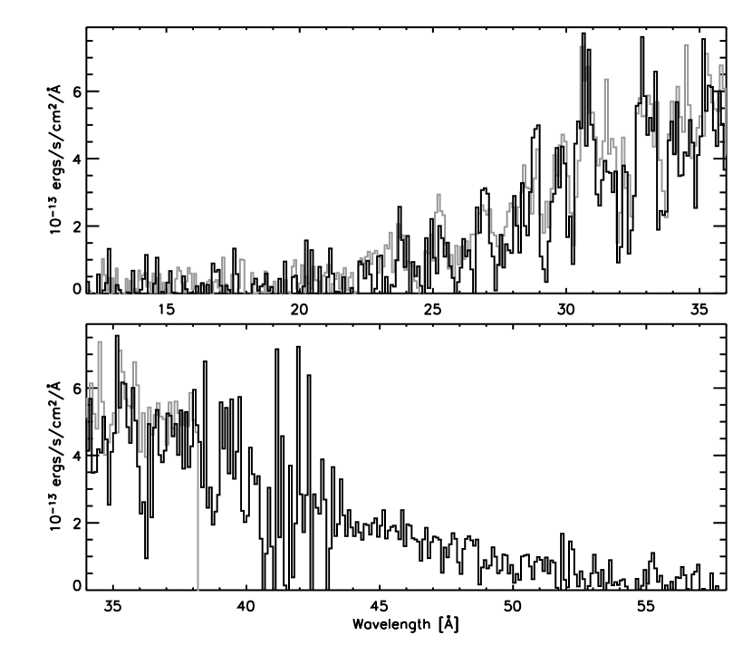
Figure 1: Chandra  LETG (black line) and XMM-Newton  RGS (grey line) spectra of CAL 83. The spectra were rebinned by a factor of 8.

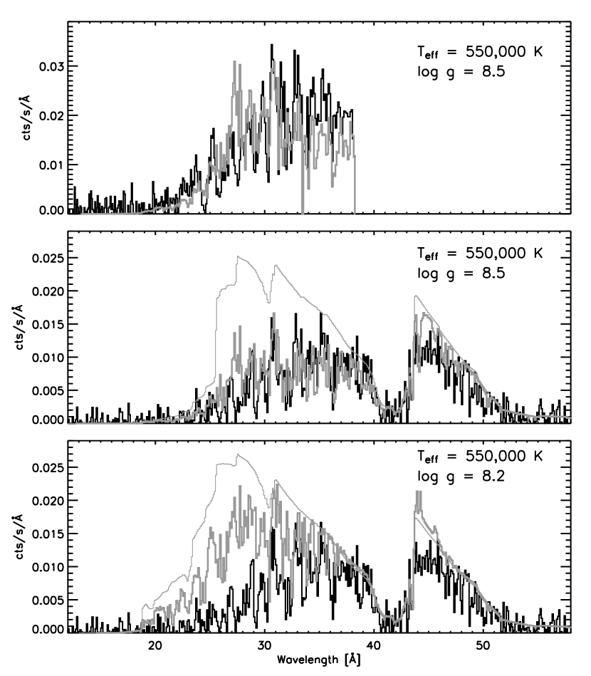
Figure 5: Best model fit to the RGS (top) and LETG (middle) spectra. The model spectrum is normalized to the LETG spectrum between 45 and 50 Å, and the same normalization is applied when matching the RGS spectrum. This normalization yields a WD radius of 0.01 $R_{\odot}$ and a WD mass of 1.3 $M_{\odot}$ (see Table 3). The bottom panel shows the model sensitivity to surface gravity, hence to the WD mass, that is here 0.65 $M_{\odot}$. The predicted continuum spectra are also shown to illustrate the importance of line opacity.

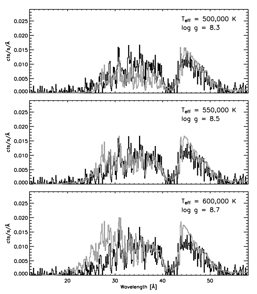
Figure 6: Comparison of the best model fit (middle panel) to the LETG spectrum with cooler (top) and hotter (bottom) models. The model spectra are normalized to the LETG spectrum between 45 and 50 Å, and the derived WD radius decreases with increasing $T_{\rm eff}$. All three models have a WD mass of about 1.3 $M_{\odot}$.

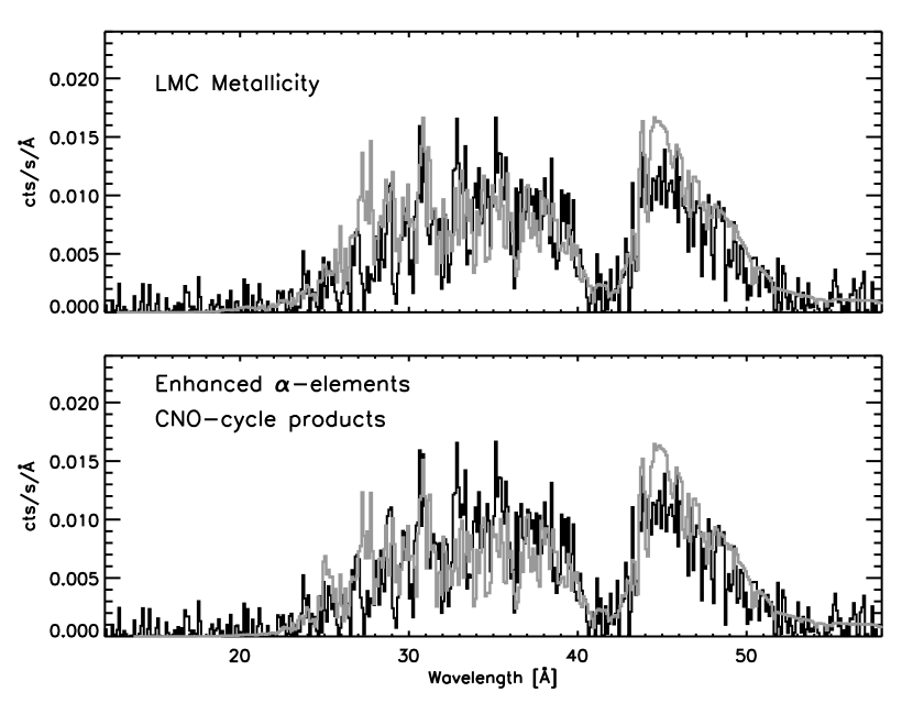
Figure 7: Best model fit to the LETG spectrum, $T_{\rm eff}$= 550,000 K, $\log g=8.5$, assuming two different surface compositions. Top: LMC metallicity (half solar); bottom: LMC metallicity with enhanced $\alpha$-element abundances and CNO abundances typical of CNO-cycle processed material.

Fig. 1 compares the RGS spectrum (we only use RGS1 data) and the LETG spectrum, calibrated in flux with the instrumental response file. We chose to rebin the spectra by a factor of 8, as the best compromise between signal-to-noise ratio and resolution, thus resulting in a resolution slightly lower than the nominal resolution. The two spectra are very similar, both in term of the spectral energy distribution and of the line features. The LETG spectrum is very noisy between 40 and 44 Å, because of the very low effective area due to instrumental (HRC-S) absorption by the carbon K edge at 43.6 Å. This instrumental absorption is clearly seen in Figs. 5-7 and is well represented in the response function applied to the NLTE model spectra.

4 X-ray Variability

Although the main scope of the Chandra  and XMM-Newton  observations were to obtain the first high-resolution X-ray spectra of CAL 83, we have extended our analysis to look for X-ray flux variations during the observations.

4.1 A New X-Ray Off-State

X-ray off-states have been rarely caught, with two exceptions in April 1996 by ROSAT (Kahabka et al., 1996) and in November 1999 by Chandra (Greiner & Di Stefano, 2002). We report here another X-ray off-state. Because of solar flare activity, our Chandra  HRC-S/LETG observation in August 2001 was interrupted after 35 ksec and rescheduled for completion in October 2001. This latter exposure, however, did not detect X-rays from CAL 83 in 62 ksec, indicating a X-ray off-state. We extracted counts at the expected position (obtained from the August Chandra LETG observation which detected CAL 83) using a circle of 1$\farcs$4 radius (95% encircled energy for the mirror point-spread function, PSF), and extracted background counts from a concentric annulus having an area 50 times larger. We obtained 34 and 1223 counts, respectively, for a 61.55 ksec exposure. We then followed the approach of Kraft et al. (1991) to determine the upper confidence limit using a Bayesian confidence level of 95%. This upper limit is 21.045 counts. Our adopted unabsorbed model spectrum (see §6.2) corresponds to $L_{\mathrm{X}}=2.7\times 10^{37}$ ergs s^-1 ($0.1-10$ keV), i.e., a zeroth order count rate of 0.10 ct s^-1 (i.e. an absorbed flux at Earth of $8.3\times 10^{-12}$ ergs s^-1 cm^-2). Consequently, the X-ray off-state corresponds to an upper limit of $L_{\mathrm{X}}<9.2\times 10^{34}$ ergs s^-1 (the upper limit of the absorbed flux at Earth is $F_{\mathrm{X}}<2.8\times 10^{-14}$ ergs s^-1 cm^-2). The upper limit on $L_{\mathrm{X}}$ is similar to that reported by Greiner & Di Stefano (2002) during the 1999 X-ray off-state. Assuming a constant bolometric luminosity, they have then infered a temperature limit, $kT\lesssim 15$ eV, that agrees well with our own estimate based on NLTE model atmospheres.

Two important caveats need to be mentioned, however. First, the extraction radius probably underestimates the encircled energy since the zeroth order PSF with LETG is not exactly similar to the mirror PSF. Thus, in principle, a larger extraction region (e.g., $3\arcsec$) should contain an encircled energy fraction closer to 100%. Since the zeroth order effective area is provided for a fraction of 100%, such a larger radius could, therefore, provide a more accurate estimate of the upper limit. Nevertheless, the second issue, that is the assumption of a similar model during the on-state and the off-state for estimating the count-to-energy conversion factor, affects the determination of the upper limit much more severely. Greiner & Di Stefano (2002) discussed several mechanisms to explain the relation between X-ray off-states and the optical variability. Since they were not able to reach a definitive conclusion, we do not know for instance if the spectrum shifts to lower energies, which thus leaves a serious uncertainty on the way of establishing an upper limit to the X-ray luminosity during the off-states. The calculated upper limit, therefore, remains indicative only.

The original 1996 off-state was interpreted in two contrasted ways. On one hand, Alcock et al. (1997) considered a model of cessation of the steady nuclear burning related to a drop in the accretion rate. The WD would need to cool quickly to explain the observed off-state, and the timescale of the off-state implies a massive WD. This model was based on the combination of optical and X-ray variability, and was later criticized by Greiner & Di Stefano (2002) who found that optical low states were delayed by about 50 days relative to the X-ray off-states. On the other hand, Kahabka (1998) argued that the off-state is caused by increased accretion resulting in the swelling and cooling of the WD atmosphere. Assuming adiabatic expansion at constant luminosity and a realistic accretion rate ($\dot{M}\approx 10^{-6}~{}M_{\odot}\,{\rm yr}^{-1}$), he argued from the characteristic timescale of the off-state that the WD is massive, $M_{\rm WD}\gtrsim 1.2M_{\odot}$.

Greiner & Di Stefano (2002) discussed extensively the X-ray off-states and optical variability of CAL 83. They believe that a cessation of nuclear burning was highly unlikely because the short turnoff time requires the WD to have a mass close to $M_{\rm CH}$, while earlier spectrum analyses (e.g., Parmar et al. 1998) suggested that the WD mass was not so high. Assuming then that the luminosity stays roughly the same, Greiner & Di Stefano investigated two ways to explain the off-states, namely an increase of the photospheric radius or absorption by circumstellar material that would in both cases shift the emission to another spectral domain. From a careful study of the variation patterns, they raised a number of issues for the two models indicating that the optical variability could not be understood with a simple model but requires some complex interaction between the photospheric expansion and the disk.

CAL 83 was considered as the prototypical CBSS undergoing steady nuclear burning. However, the observation of a third off-state now demonstrates the recurrent nature of the phenomenon in CAL 83. We defer further discussion on the origin of the off-states after the spectrum analysis.

4.2 Long-Term and Short-Term Time Variability

Figure 2 shows the light curves of CAL 83 with XMM-Newton  (EPIC pn: top panel, RGS: middle panel) and Chandra (LETG1: bottom panel) in units of flux observed at Earth. We use our final model spectrum in combination with the respective response matrices to obtain conversion factors. Note that, in the case of EPIC pn, the observation was cut into three pieces of similar length but using different filters. To avoid pile-up and optical contamination, we extracted EPIC events in an annulus ($0.2-0.8$ keV range), and used a nearby region for the background. In the case of RGS and LETG, the background was obtained from events “above” and “below” the dispersed spectrum. We used events in the range $20-37$ Å  for RGS, and $20-65$ Å  for LETG, since no signal was present outside these ranges.

Although the absolute observed flux still contains some uncertainty (e.g., cross-calibration between instruments, imperfect model), similar flux levels were obtained during both the XMM-Newton and Chandra  observations, despite their time separation of $1.25$ yr. Greiner & Di Stefano (2002) also noted that the flux observed by XMM-Newton  was comparable to earlier observations with ROSAT and BeppoSAX. Not only the flux levels were the same, but we found that the RGS and the LETG spectra were remarkably similar (Fig. 1). On the other hand, we have detected relative, short-timescale variations in the X-ray light curves. Their typical timescale is much shorter than the 1.04-day binary orbital period. These flux variations can reach up to 50% of the average flux. Hardness ratios light curves do not show significant variations, suggesting that the flux variations are not due to temperature fluctuations. However, because of the limited signal-to-noise ratio due to the small effective areas, we stress that we cannot exclude that temperature effects played some role in the flux variations. Simultaneous UV and optical photometry with a similar time sampling would be necessary to study stochastic effects in the accretion process.

5 NLTE Model Atmospheres

We have constructed a series of NLTE line-blanketed model atmospheres of hot WD’s with our model atmosphere program, TLUSTY, version 201. Detailed emergent spectra are then calculated with our spectrum synthesis code, SYNSPEC, version 48, using the atmospheric structure and the NLTE populations previously obtained with TLUSTY. TLUSTY computes stellar model photospheres in a plane-parallel geometry, assuming radiative and hydrostatic equilibria. Departures from LTE are explicitly allowed for a large set of chemical species and arbitrarily complex model atoms, using our hybrid Complete Linearization/Accelerated Lambda Iteration method (Hubeny & Lanz, 1995). This enables us to account extensively for the line opacity from heavy elements, an essential feature as the observed spectrum is suggestive of strong line opacity (see Fig. 1).

We have implemented in our two codes several specific upgrades for computing very hot model atmospheres as well as detailed X-ray spectra. Starting with version 200, TLUSTY is a universal code designed to calculate the vertical structure of stellar atmospheres and accretion disks. With this unification, we directly benefit from the upgrades implemented to calculate very hot accretion disk annuli. This concerns in particular a treatment of opacities from highly ionized metals and Compton scattering (Hubeny et al., 2001).

Originally, Hubeny et al. (2001) implemented a simple description of metal opacities to explore the basic effect of these opacity sources on accretion disk spectra. Adopting one-level model atoms, they treated all ions, from neutrals to fully stripped atoms, of the most abundant chemical species: H, He, C, N, O, Ne, Mg, Si, S, Ar, Ca, and Fe. Therefore, only photoionization from the ground state of each ion is considered. Photoionization cross-sections, including Auger inner-shell photoionization, were extracted from the X-ray photoionization code XSTAR (Kallman, 2000). We made the simplifying assumption that, if an Auger transition is energetically possible, then it occurs and the photoionization results in a jump by two stages of ionization to a ground state configuration. Fluorescence and multiple Auger electron ejection arising from inner shell photoionization are neglected. To handle dielectronic recombination, we followed the description of Hubeny et al. (2001), based on data from Aldrovandi & Péquignot (1973), Nussbaumer & Storey (1983), and Arnaud & Raymond (1992), which are used in XSTAR.

These models only include bound-free opacities from the ground states. Therefore, we constructed multi-level model atoms in order to account for the effect of metal lines in our NLTE model atmospheres. We did so only for the most populated ions, and ions with very low populations are excluded. We retained the ionization and recombination data discussed above for ground state levels, and expanded the model atoms using data calculated by the Opacity Project (OP, 1995, 1997). It is essential to explicitly incorporate highly-excited levels in the model atoms, because X-ray lines (where the model atmosphere flux is maximal) are transitions between low-excitation (or ground state) and these highly-excited levels. To deal with the large number of excited levels, we merged levels with close energies into superlevels assuming that they follow Boltzmann statistics relative to each other (that is, all individual levels in a superlevel share the same NLTE departure coefficient). Proper summing of individual transitions is applied for transitions between superlevels. Refer to Hubeny & Lanz (1995) and Lanz & Hubeny (2003) for details on NLTE superlevels and on the treatment of transitions in TLUSTY. Table 2 lists the ions included in the model atmospheres, the number of explicit NLTE levels and superlevels, and the corresponding numbers of superlevels and lines. We recall here that OP neglected the atomic fine structure, and these figures refer to OP data (hence, the actual number of levels and lines accounted for is higher by a factor of a few). For each ion, we list the original publications unless the calculations were only published as a part of the OP work. Data for one-level model atoms are from Kallman (2000).

The second upgrade in TLUSTY deals with electron scattering, and we have considered the effect of Compton vs. Thompson scattering. At high energies, Compton scattering provides a better physical description. Compton scattering is incorporated in the radiative transfer equation in the nonrelativistic diffusion approximation through a Kompaneets-like term. Details of the implementation are described in Hubeny et al. (2001). Through a coupling in frequencies, this increases significantly the computational cost. We thus decided to explore the differences resulting from using Compton or Thompson scattering. We performed a small number of tests comparing model atmospheres and predicted spectra which were computed using these two approaches. At the considered temperatures ($T\approx 500,000$ K), the differences are very small and become visible only in the high-energy tail, above 2 keV. At these energies, the predicted flux is very low and, indeed, no flux has been observed in CBSS at these energies. Moreover, the changes result in little feedback on the calculated atmospheric structure. We may therefore safely use Thompson scattering in modeling CBSS atmospheres.

Detailed spectra are produced in a subsequent step with our spectrum synthesis program SYNSPEC, assuming the atmospheric structure and NLTE populations calculated with TLUSTY. Upgrades made in the TLUSTY program have been transported in SYNSPEC when necessary. A detailed line list for the soft X-ray domain was built, combining essentially two sources. The initial list was extracted from Peter van Hoof Atomic Line List. This list contains transitions between levels with measured energies, and all lines thus have accurate wavelengths. These lines represent, however, a small fraction of all lines in the soft X-ray range because the energy of most highly-excited levels has not been measured from laboratory spectra. We thus complemented this initial list with a complete list of transitions from OP. The OP lines do not account for fine structure, and wavelengths are derived from theoretical energies. The expected accuracy of the theoretical wavelengths is expected to be of the order of 0.5 Å  or better. This is, however, not as good as the spectral resolution achieved with Chandra or XMM-Newton spectrometers, and potential difficulties may be expected when comparing model spectra to observations. Yet the global opacity effect of these lines is important. The line list only contains lines from the explicit NLTE ions. The spectra are calculated using the NLTE populations from the TLUSTY models, and SYNSPEC does not require partition functions in this case. Finally, we examined the issue of line broadening. As discussed by Mihalas (1978), natural broadening becomes the main effect for lines of highly-charged ions, and already dominates the linear Stark broadening for C VI lines. Therefore, we included natural broadening data when available, and we neglected Stark broadening.

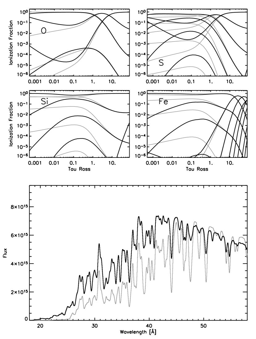
Figure 3: Ionization fractions and predicted spectra of a NLTE (black lines) and a LTE (grey lines) model atmosphere, $T_{\rm eff}$= 550,000 K, $\log g=8.5$. The top part shows the ionization fractions of O, Si, S and Fe. Dominant ions in the line formation region ($\tau_{\rm Ross}\approx 0.1-0.01$) are O VII, Si XIII, S XIII and Fe XVII. LTE and NLTE predicted spectra, convolved to a 0.3 Å  resolution, are compared in the bottom panel.

Departures from LTE are illustrated in Fig. 3 for a model atmosphere with $T_{\rm eff}$  = 550,000 K, $\log g=8.5$, and a LMC metallicity. The ionization fractions show that the NLTE model is overionized compared to the LTE model, which is a typical behavior of NLTE model stellar atmospheres where the radiation temperature is higher than the local electronic temperature. As expected, the NLTE ionization fractions return to their LTE values at depth ($\tau_{\rm Ross}\gtrsim 2$). The overionization remains limited because the local temperatures are higher in the LTE model compared to the NLTE model as a result of stronger continuum and line absorption at depths around $10^{-3}\lesssim\tau_{\rm Ross}\lesssim 1$. This stronger absorption is indeed visible in the predicted emergent spectrum: the LTE predicted flux is significantly lower below 45 Å. Deriving a lower surface gravity, hence a lower WD mass, would therefore be a consequence of a LTE analysis compared to the NLTE analysis (see also §6.2 and Fig. 5).

6 Spectrum Analysis

6.1 Methodology

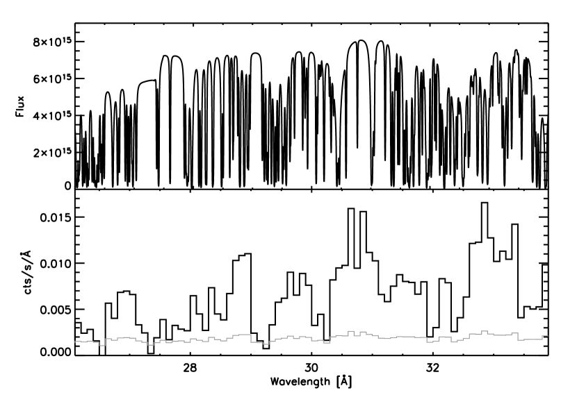
Figure 4: Comparison of the observed spectral resolution in the Chandra  LETG spectrum (bottom panel; observed counts s^-1 Å^-1) with the best fit model spectrum (top panel; flux at the stellar surface in ergs s^-1 cm^-2 Å^-1), demonstrating that the observed spectral features are blends of many metal lines. The 1-$\sigma$ count rate error is shown in the bottom panel (thin grey line) allowing to assess whether the observed spectral features are genuine or not.

We display in Fig. 4 a typical spectral region of the Chandra  LETG data together with the predicted spectrum of the stellar surface, that is without any instrumental convolution. This clearly illustrates that all observed features are actually blends of many metal lines, mostly from Si XII, S XI, S XII, Ar X, Ar XI, Ar XII, Ca XII, and Fe XVI. It is thus impractical to identify these features individually. Moreover, the fact that we had to use theoretical wavelengths for many predicted lines compounds the difficulties. Therefore, the spectrum analysis cannot be based on fitting a few key features to derive the properties of CAL 83, but we rather need to achieve an overall match to the observed spectrum. To this end, we do not use any statistical criterion but we simply match the model to the data by eye. A $\chi^{2}$ statistics would primarily measure the line opacity that is missing in the model (a systematic effect) rather than efficiently discriminate between different values of the stellar parameters (see §6.2). Errors are analogously estimated by eye, that is, models outside the error box clearly exhibit a poor match to the observations. We feel that this approach provides conservative error estimates.

We started from the stellar parameters derived by Paerels et al. (2001), and built a small grid of NLTE model atmospheres around these initial estimates covering a range in effective temperature and surface gravity, $450,000\lesssim T_{\rm eff}\lesssim 600,00$ K and $8\lesssim\log g\lesssim 9$. For each set of parameters, we constructed the final model in a series of models of increasing sophistication, adding more explicit NLTE species, ions, levels, and lines. Table 2 lists the explicit species included in the final models. This process was helpful numerically to converge the models, but this was primarily used to investigate the resulting effect on the predicted spectrum of incorporating additional ions in the model atmospheres. We have assumed that the surface composition of CAL 83 reflects the composition of the accreted material, i.e. typical of the LMC composition. We have adopted a LMC metallicity of half the solar value (Rolleston et al., 2002). Additional models with a composition reflecting an evolved star donor with CNO-cycle processed material and enhanced $\alpha$-element abundances have also been calculated to explore the effect of changing the surface composition on the derived stellar parameters.

To compare the model spectra to the Chandra  LETG and XMM-Newton  RGS data, we applied to the model a correction for the interstellar (IS) extinction, the appropriate instrumental response matrix (see §3), and a normalization factor $(R_{\rm WD}/d)^{2}$.

Our IS model is based on absorption cross-sections in the X-ray domain compiled by Balucinska-Church & McCammon (1992) for 17 astrophysically important species. Specifically, the effective extinction curve was calculated with Balucinska-Church & McCammon’s code, assuming a solar abundance mix (Grevesse & Sauval, 1998). The total extinction is then proportional to the hydrogen column density. We used the value, $N_{\rm H}=6.5\pm 1.0~{}10^{20}$ cm^-2, measured by Gänsicke et al. (1998) from Ly $\alpha$ HST GHRS observations of CAL 83.

After the IS extinction and instrumental corrections, the model spectra were scaled to the Chandra  LETG spectrum to match the observed flux level longward of 45 Å, yielding the normalization factor $(R_{\rm WD}/d)^{2}$. The WD radius immediately follows from the adopted distance to the LMC, $d=50\pm 3$ kpc, based on RR Lyrae and eclipsing binaries (Alcock et al., 2004; Clausen et al., 2003).

6.2 Results and Discussion

We present in Fig. 5 and 6 our best model fit to the RGS and LETG spectra along with the model sensitivity to $T_{\rm eff}$  and $\log g$. The best model spectrum has been normalized to match the observed LETG flux between 45 and 50 Å, yielding a WD radius of $R_{\rm WD}=7.3~{}10^{8}$ cm $\approx 0.01\,R_{\odot}$. The same normalization factor is then applied for comparing the model spectrum to the RGS spectrum. The benefit of having a broader spectral coverage with LETG is instantly apparent for deriving an accurate model normalization. The top two panels of Fig. 5 generally show a satisfactory agreement between the model and the two observed spectra. Above 34 Å, the match to the RGS spectrum is not as good as for the LETG spectrum, probably resulting from the difficulty of correcting the RGS data for fixed-pattern noise in this range. The general energy distribution and most spectral features are well reproduced, for instance the features at 24, 29, 30, 32, and 36 Å. On the other hand, the observed absorption at $\approx$ 27 Å  is not reproduced by our model. A cursory look might suggest that the model predicts an emission feature there but, overplotting the predicted continuum flux, we see that the model essentially misses line opacity around 27-28 Å. In this respect, our analysis definitively demonstrates that we observe a photospheric absorption spectrum, with no obvious evidence of emission lines.

Fig. 5 presents two models with a different surface gravity, clearly demonstrating that our data allow us to determine $\log g$. The higher flux in the low gravity model is the result of a higher ionization in the low gravity model atmosphere, decreasing the total opacity in the range between 20 and 30 Å. This effect is large enough to determine the surface gravity with a good accuracy, typically $\pm~{}0.1$ dex on $\log g$. Fig. 6 shows three models with different effective temperatures. The surface gravity was adjusted to provide the closest match to the observed spectrum, and the appropriate model normalizations and WD radii were determined. The differences between the models are not as large as in the case of gravity, but we may exclude models as cool as 500,000 K or as hot as 600,000 K. We thus adopt $T_{\rm eff}$ = 550,000 $\pm$ 25,000 K ($k$$T_{\rm eff}$ = 46 $\pm$ 2 eV). The WD mass and luminosity straightforwardly follow, and our results are summarized in Table 3. Uncertainties are propagated as dependent errors, formally yielding a WD mass of $M_{\rm WD}=1.3\pm 0.3M_{\odot}$. The mass-radius relation for cold WD’s predicts a WD radius of about 0.004 $R_{\odot}$ for such a high WD mass (Hamada & Salpeter, 1961), implying that CAL 83 has a swollen atmosphere with a measured radius 2.5 times the expected value. Kato (1997) calculations of WD envelopes predict an even larger radius ($\approx 0.025R_{\odot}$) for the derived mass and temperature, suggesting that the observed emission may emerge only from a hot cap on the WD surface. The derived bolometric luminosity, $L_{\rm bol}=3.5\pm 1.2~{}10^{37}$ ergs s^-1, is higher than the luminosity range given by Gänsicke et al. (1998) but consistent with Kahabka (1998) estimate, and corresponds to about 0.3 $L_{\rm Edd}$.

The surface composition of WD’s in CBSS is yet unknown. It might reflect either the composition of the accreted material or the nucleosynthetic yields of nuclear burning close to the WD surface. Characterizing this composition would be of major interest for understanding the physical processes occurring on the accreting WD. However, our first concern is to verify how sensitive the determination of stellar parameters is with respect to the assumed composition. So far, we have assumed a composition typical of the LMC metallicity. If the donor star has already evolved off the main sequence, its surface composition might already be altered and might show enhanced abundances of $\alpha$ elements and/or CNO abundances resulting from the mixing with CNO-cycle processed material. We have therefore constructed a NLTE model atmosphere, assuming the same effective temperature and surface gravity, but all $\alpha$ elements are overabundant by a factor of 2, carbon (1/50 the LMC abundance) and oxygen (1/5) are depleted, and nitrogen (8 times) is enhanced. Fig. 7 compares the match of the two models to the LETG spectrum. A careful examination shows that indeed the model with the altered composition reveals some stronger absorption lines, but the changes remain small. We conclude first that the determination of the stellar parameters is little affected by the assumed surface composition (within some reasonable range; exotic compositions will not match the observations), and second that a detailed chemical composition analysis would require improved atomic data.

Velocities are a further factor affecting the strength of the absorption line spectrum. In particular, we adopted a microturbulent velocity of 50 km s^-1. The ratio of this value to the sound speed is rather typical of values derived in other hot stars. Nevertheless, we varied the microturbulent velocity from low values up to values close to the sound velocity to investigate the effect of different microturbulences on the predicted spectrum. The line absorption spectrum indeed strengthened at larger microturbulent velocities, but the overall match to the LETG data is not much changed. The derived parameters remain, therefore, insensitive to the assumed microturbulent velocity. We also explored the role of an outflow in strengthening and broadening the spectral lines because of the presence of a strong wind from the WD has been proposed to regulate the accretion (Hachisu et al., 1996). We carefully examined the LETG spectrum, using different binning factors. We did not find evidence of emission or line asymmetries that could reveal an outflow. Note, however, that the spectral resolution would only allow us to detect fast outflows ($>$2000 km s^-1). For the same reason, we can only exclude very fast apparent rotation velocities, e.g., values close to the critical velocity ($\approx$ 7000 km s^-1). It is likely, however, that the inclination angle of the WD rotation axis is small because the absence of eclipses indicates that the accretion disk is almost seen face-on. Therefore, our observations cannot rule out a fast WD rotation which is advocated by Yoon et al. (2004) for the WD to gain mass efficiently.

The uncertainty on the IS transmission might be the most severe issue. Our IS model (see §6.1) predicts a transmission as low as 6% at 50 Å increasing up to about 60% at 20 Å. A change in the assumed hydrogen column density toward CAL 83 might thus significantly affect the results. Fortunately, this column was measured accurately from Ly $\alpha$ observations by Gänsicke et al. (1998), $N_{\rm H}=6.5\pm 1.0~{}10^{20}$ cm^-2. We use their error range to explore the resulting changes. Thanks to the relatively tight range, the spectral shape between 25 and 40 Å  is little changed, and stays within changes predicted from the adopted errors on $T_{\rm eff}$  and $\log g$. Therefore, the error on the column density primarily translates into different normalization factors, i.e. a range of WD radii. A higher column density yields a larger WD radius, hence a larger WD mass (which should not exceed $M_{\rm CH}$). Conversely, a smaller column density yields a lower WD radius, hence a lower luminosity. Since the measured luminosity is close the boundary of stable steady-state nuclear burning (Iben, 1982; van den Heuvel et al., 1992), it is unlikely that the WD luminosity is much smaller. Therefore, the actual value of the IS density column likely is within an even tighter range. The uncertainty on the WD radius listed in Table 3 remains relatively small, because it only combines the uncertainty on the normalization factor and on the LMC distance which are well determined. Fully accounting for Gänsicke et al. (1998) error bar on $N_{\rm H}$ would translate to unrealistically large errors on the WD radius and on the WD mass.

We revisit now the issue of the X-ray off-states in the light of our result that the WD has a high mass. Kato (1997) calculations of WD envelopes showed that the X-ray turnoff time after the cessation of nuclear burning could be very short for massive WDs. An observed turnoff time as short as 20 days (Kahabka, 1998) implies $M_{\rm WD}\gtrsim 1.35M_{\odot}$. Gänsicke et al. (1998) noted that CAL 83 has a low luminosity for a CBSS and is found close to the stability limit of steady burning, which is thus consistent with the idea of unstable burning and might also be related to our discovery of short term variability of the X-ray flux. Although the actual process responsible of the off-states cannot be definitively established, the characteristic timescale supports the idea of a massive WD in CAL 83.

7 Conclusions

Table 3 summarizes our results. Our spectroscopic analysis indicates that CAL 83 contains a massive WD, $M_{\rm WD}=1.3\pm 0.3M_{\odot}$. Obviously, the upper limit is well over $M_{\rm CH}$, but a more interesting issue to tie CBSS and SN Ia progenitors is the lower limit for the mass. Because low-mass models do not provide a match to the observed spectrum that is as good as the fits achieved with high-mass models, we have concluded that $M_{\rm WD}>1.0~{}M_{\odot}$ is a robust lower limit for the WD mass. Nevertheless, we need to emphasize here that this conclusion depends on our current description of the soft X-ray opacities, particularly between 20 and 40 Å. We believe that the OP data already provide a good description and, although progress in this regard would be very helpful, we do not expect changes drastic enough to modify our conclusion. The issue of IS extinction is potentially more serious, but we have argued that we have an accurate estimate of the hydrogen column density toward CAL 83. In addition, our model is consistent with the WD surface having a hydrogen-rich composition with LMC metallicity. Finally, our analysis does not reveal any evidence of an outflow from the WD.

We have reported a third X-ray off-state, showing that CAL 83 is a source undergoing unstable nuclear burning. This is consistent with its low luminosity. The short timescale of the off-states (about 50 days) provides a supporting evidence that CAL 83 WD is massive ($M_{\rm WD}\gtrsim 1.35M_{\odot}$). A better characterization of the off-states is required to definitively establish the mechanism(s) responsible of the off-states. Moreover, we confirm that the X-ray luminosity is fairly constant on a long-term basis during on-states. However, on the other hand, we found variations up to 50% of the soft X-ray luminosity in very short times (less than 0.1 orbital period). Simultaneous X-ray and optical photometry covering continuously a duration longer than a full orbital period would be very valuable to study stochastic accretion processes.

Within the model of SN Ia progenitors proposed by Hachisu et al. (1996), our results would place CAL 83 in a late stage, after the strong accretion and wind phase when the accretion rate drops below the critical rate for sustaining steady nuclear burning. Our results therefore make CAL 83 a very likely candidate for a future SN Ia event. We plan to conduct a similar NLTE analysis of the few other CBSS already observed with Chandra  LETG spectrometer to further support our results and quantitatively study differences between these objects. In particular, the second typical CBSS, CAL 87, exhibits a very different spectrum characterized by emission lines (Greiner et al., 2004). A detailed spectroscopic analysis should reveal either if the different spectrum arises from a different geometry (edge-on vs. face-on system) or if CAL 87 is in an earlier evolutionary stage.

Figure 2: X-Ray light curves of CAL 83 built from XMM-Newton  EPIC pn (top panel), RGS (middle panel), and Chandra  HRC-S/LETG1 observations. Note the short-timescale variability, while the flux level remains the same between the XMM-Newton  and the Chandra  observations.

Table 1: Chandra  and XMM-Newton  Observation Log of CAL 83.

Mission	Instrument	Exp. Time	Start Time	End Time	State
Chandra	HRC-S/LETG	52.3 ksec	1999-11-29 06:33	1999-11-29 21:27	Off-state
Chandra	ACIS-S	2.1 ksec	1999-11-30 14:50	1999-11-30 15:47	Off-state
XMM-Newton	RGS & EPIC	45.1 ksec	2000-04-23 07:34	2000-04-23 20:04
Chandra	HRC-S/LETG	35.4 ksec	2001-08-15 16:03	2001-08-16 02:10
Chandra	HRC-S/LETG	61.6 ksec	2001-10-03 11:35	2001-10-04 05:12	Off-state

Table 2: Atomic data included in the NLTE model atmospheres.

Ion	(Super)Levels	Indiv. Levels	Lines	References
H I	9string	80string	172string
H II	1string	1string
He II	15string	15string	105string
He III	1string	1string
C V	9string	19string	27string	stringFernley et al. (1987)
C VI	15string	15string	105string
C VII	1string	1string
N V	5string	14string	28string	stringPeach et al. (1988)
N VI	9string	19string	27string	stringFernley et al. (1987)
N VII	15string	15string	105string
N VIII	1string	1string
O V	1string	1string
O VI	8string	20string	60string	stringPeach et al. (1988)
O VII	13string	41string	107string	stringFernley et al. (1987)
O VIII	15string	15string	105string
O IX	1string	1string
Ne V	1string	1string
Ne VI	1string	1string
Ne VII	1string	1string
Ne VIII	5string	14string	28string	stringPeach et al. (1988)
Ne IX	9string	19string	27string	stringFernley et al. (1987)
Ne X	15string	15string	105string
Ne XI	1string	1string
Mg IX	1string	1string
Mg X	12string	54string	284string	stringPeach et al. (1988)
Mg XI	15string	109string	565string	stringFernley et al. (1987)
Mg XII	1string	1string
Si IX	22string	489string	11900string	stringLuo & Pradhan (1989)
Si X	24string	313string	7531string	stringOP (1995)
Si XI	16string	184string	2599string	stringTully et al. (1990)
Si XII	12string	54string	284string	stringPeach et al. (1988)
Si XIII	9string	19string	27string	stringFernley et al. (1987)
Si XIV	1string	1string
S IX	20string	481string	13665string	stringOP (1995)
S X	23string	512string	17966string	stringOP (1995)
S XI	23string	587string	16253string	stringLuo & Pradhan (1989)
S XII	23string	301string	7181string	stringOP (1995)
S XIII	13string	184string	2599string	stringTully et al. (1990)
S XIV	12string	54string	284string	stringPeach et al. (1988)
S XV	9string	19string	27string	stringFernley et al. (1987)
S XVI	1string	1string
Ar VIII	1string	1string
Ar IX	23string	197string	2877string	stringOP (1995)
Ar X	19string	287string	6836string	stringOP (1995)
Ar XI	20string	514string	15943string	stringOP (1995)
Ar XII	22string	546string	21675string	stringOP (1995)
Ar XIII	26string	617string	19248string	stringLuo & Pradhan (1989)
Ar XIV	19string	355string	9755string	stringOP (1995)
Ar XV	16string	184string	2599string	stringTully et al. (1990)
Ar XVI	1string	1string
Ca IX	1string	1string
Ca X	1string	1string
Ca XI	24string	203string	3098string	stringOP (1995)
Ca XII	15string	308string	8043string	stringOP (1995)
Ca XIII	26string	544string	17703string	stringOP (1995)
Ca XIV	22string	629string	27835string	stringOP (1995)
Ca XV	24string	730string	24897string	stringLuo & Pradhan (1989)
Ca XVI	21string	381string	11511string	stringOP (1995)
Ca XVII	1string	1string
Ca XVIII	1string	1string
Ca XIX	1string	1string
Fe XIII	1string	1string
Fe XIV	1string	1string
Fe XV	26string	253string	4797string	stringButler et al. (1993)
Fe XVI	17string	52string	285string	stringOP (1995)
Fe XVII	30string	211string	3409string	stringOP (1995)
Fe XVIII	1string	1string
Fe XIX	1string	1string
Fe XX	1string	1string
Fe XXI	1string	1string
Fe XXII	1string	1string
Fe XXIII	1string	1string
Fe XXIV	1string	1string
Fe XXV	1string	1string

Table 3: Stellar Parameters of CAL 83.

Effective Temperaturestring	$T_{\rm eff}=5.5\pm 0.25~{}10^{5}$ K
Surface Gravity	$\log g=8.5\pm 0.1$ (cgs)
WD Radius	$R_{\rm WD}=0.01\pm 0.001~{}R_{\odot}$
WD Luminosity	$L_{\rm WD}=9\pm 3~{}10^{3}~{}L_{\odot}$
WD Mass	$M_{\rm WD}=1.3\pm 0.3~{}M_{\odot}$

References

- Alcock et al. (1997) Alcock, C., Allsman, R. A., Alves, D., et al. 1997, MNRAS, 286, 483
- Alcock et al. (2004) Alcock, C., Alves, D. R., Axelrod, T. S., et al. 2004, AJ, 127, 334
- Aldrovandi & Péquignot (1973) Aldrovandi, S. M. V., & Péquignot, D. 1973, A&A, 25, 137
- Arnaud & Raymond (1992) Arnaud, M., & Raymond, J. 1992, ApJ, 398, 394
- Arnett (1969) Arnett, D. W. 1969, Ap&SS, 5, 180
- Balucinska-Church & McCammon (1992) Balucinska-Church, M., & McCammon, D. 1992, ApJ, 400, 699
- Butler et al. (1993) Butler, K., Mendoza, C., & Zeippen, C. J. 1993, J. Phys. B, 26, 4409
- Cassisi et al. (1998) Cassisi, S., Iben, I. Jr., & Tornambè, A. 1998, ApJ, 496, 376
- Clausen et al. (2003) Clausen, J. V., Storm, J., Larsen, S. S., & Giménez, A. 2003, A&A, 402, 509
- Cowley et al. (1984) Cowley, A. P., Crampton, D., Hutchings, J. B., et al. 1984, ApJ, 286, 196
- Dreizler & Werner (1993) Dreizler, S., & Werner, K. 1993, A&A, 278, 199
- Fernley et al. (1987) Fernley, J. A., Taylor, K. T., & Seaton, M. J. 1987, J. Phys. B, 20, 6457
- Gänsicke et al. (1998) Gänsicke, B. T., van Teeseling, A., Beuermann, K., & de Martino, D. 1998, A&A, 333, 163
- Greiner et al. (1991) Greiner, J., Hasinger, G., & Kahabka, P. 1991, A&A, 246, L17