Deconvolution Map-Making for Cosmic Microwave Background Observations

Abstract

We describe a new map-making code for cosmic microwave background (CMB) observations. It implements fast algorithms for convolution and transpose convolution of two functions on the sphere (Wandelt & Górski 2001) WG01 . Our code can account for arbitrary beam asymmetries and can be applied to any scanning strategy. We demonstrate the method using simulated time-ordered data for three beam models and two scanning patterns, including a coarsened version of the WMAP strategy. We quantitatively compare our results with a standard map-making method and demonstrate that the true sky is recovered with high accuracy using deconvolution map-making.

I Introduction

Real microwave telescopes collect distorted information about the cosmic microwave background (CMB) anisotropies due to asymmetries in the beam shape AAS02 and stray light from sources such as the Galaxy B00 ; B03 . To correct for these systematic errors we must be able to remove the detector response at all orientations of the telescope over the whole sky. In an optimal treatment, this correction must be applied during the map-making step of the CMB data analysis pipeline, before the angular power spectrum can be reconstructed. The problem becomes increasingly important as new generations of CMB observations probe for ever fainter signals in the CMB sky, and especially as we are preparing to measure the polarization of the CMB with high sensitivity. We present a complete map-making algorithm, in which time-ordered data (TOD) is used to construct a temperature map and beam distortions are removed.

We call our approach deconvolution map-making, a generalization of existing CMB map-making techniques to solve the maximum likelihood map-making problem for arbitrary beam shapes. For sufficiently high signal-to-noise this technique allows super-resolution imaging of the CMB from time-ordered scans. We implement our method using the exact algorithms for the convolution and transpose convolution of two arbitrary function on the sphere – in this case the sky and the beam – as detailed by Wandelt and Górski in WG01 . These fast methods for convolution and transpose convolution are efficient because they make use of the Fast Fourier Transform algorithm. They are guaranteed to work to numerical precision for band-limited functions on the sphere.

Early work on the map-making problem have relied on the brute force method of direct matrix inversion. However, current and future CMB experiments, like the Wilkinson Microwave Anisotropy Probe (WMAP) WMAP and Planck satellite Planck , return enormous data sets that render the brute force method useless. More recent advancements include map-making methods applicable to the latest experiments; however, many treat the beam like a perfect delta-function (e.g. D01 ; YM04 ) or assume a symmetric beam profile (e.g. N01 ), and thereby relegate the problem of treating a non-Gaussian radial response of the beam to subsequent stages in the data analysis mapmaking . In this class, special techniques exist to deal with differential measurements like that of the Differential Microwave Radiometer (DMR) on the Cosmic Background Explorer (COBE) satellite lineweaver or WMAP WMAPmaking . A Fourier method has been developed AS00 to perform deconvolution but only for non-rotating asymmetric beams. Lastly, BS03 present a method to remove the main beam distortion over patches of the sky for asymmetric, rotating beams but operate in pixel-space which is computationally more expensive than spherical-harmonic-space algorithms for the same level of accuracy WG01 ; C01 .

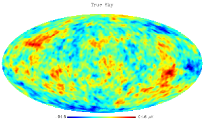
We test our algorithm on a simulated foreground- and Galaxy-free sky using a standard $\Lambda$CDM power spectrum and simulated spherical harmonic multipoles $a_{\ell m}$ up to $\ell=128$. We also use the first-year WMAP Ka-band temperature map as our true sky containing Galactic emission.

In section II we present the deconvolution method and briefly review a standard map-making method. In section III we detail the various test cases. Our results for the deconvolution method are given, discussed, and compared with the standard estimates in section IV. We conclude in section V and remark on future directions.

II Deconvolution Map-Making

In order to define our notation we will briefly review the path from observations to maps. A microwave telescope scans the CMB sky according to some scanning strategy, effectively convolving the true sky with a beam function, and returns a vector, $\mathbf{d}$, containing the $n_{TOD}$ samples of the time-ordered data. We represent this by

$$\mathbf{A}\mathbf{s}=\mathbf{d},$$ (1)

where $\mathbf{A}$ is the observation matrix, defined below, and $\mathbf{s}$ is a $n_{pix}$-vector containing the true sky.

The matrix $\mathbf{A}$ encodes both the scanning strategy and the optics of the CMB instrument. Each sample of the TOD is modeled as the scalar product of a row of the matrix $\mathbf{A}$ with the sky $\mathbf{s}$. Each of the $n_{TOD}$ rows of $\mathbf{A}$ contains a rotated map of the beam. In a given row the beam rotation corresponds to the orientation of the antenna at the point in time when the sample is taken. We will assume the beam shape and pointing of the satellite to be known.

The observation matrix $\mathbf{A}$ generalizes the notion of the pointing matrix which is often used in expositions of map-making algorithms by including both optics and scanning strategy. This generalization is necessary for any map-making method that accounts for beam functions with azimuthal structure.

The least-squares estimate of the true sky, $\mathbf{\hat{s}}$, is given by

$$\mathbf{A}^{\mathrm{T}}\mathbf{A}\mathbf{\hat{s}}=\mathbf{A}^{\mathrm{T}}\mathbf{d}.$$ (2)

The coefficient matrix in this system of equations, $\mathbf{A}^{\mathrm{T}}\mathbf{A}$, is a smoothing matrix and hence ill-conditioned. Inverting it to solve Eq. (2) therefore poses a problem.

We describe here a regularization technique for dealing with this problem. We split off the ill-conditioned part of $\mathbf{A}$ by factoring the convolution operator into $\mathbf{A}=\mathbf{BG}$ where $\mathbf{G}$ is a simple Gaussian smoothing matrix, represented in harmonic-space by

$$G_{\ell}=\rm{exp}\left(\frac{-\sigma^{2}\ell(\ell+1)}{2}\right),$$ (3)

where $\sigma=\mathrm{FWHM}/\sqrt{8\ln 2}$.

Substituting the factorization into Eq. (2), we get

$$\mathbf{G}^{\mathrm{T}}\mathbf{B}^{\mathrm{T}}\mathbf{B}\mathbf{G}\mathbf{\hat{s}} = \mathbf{G}^{\mathrm{T}}\mathbf{B}^{\mathrm{T}}\mathbf{d}$$ (4)

$$\mathbf{B}^{\mathrm{T}}\mathbf{B}\mathbf{x} = \mathbf{B}^{\mathrm{T}}\mathbf{d}$$ (5)

where we are solving for $\mathbf{x}=\mathbf{G\hat{s}}$ so as not to reconstruct the sky at higher resolution than that of the instrument.

Equation (2) is exact if the noise is stationary and uncorrelated in the time-ordered domain. For a more general noise covariance matrix in the time-ordered domain, $\mathbf{N}$, the normal equation is modified as follows

$$\mathbf{A}^{\mathrm{T}}\mathbf{N}^{-1}\mathbf{A}\mathbf{\hat{s}}=\mathbf{A}^{\mathrm{T}}\mathbf{N}^{-1}\mathbf{d}.$$ (6)

We proceed, considering only white noise in this paper; however, it is straightforward to generalize to non-white noise as indicated in Eq. (6). Indeed, the matrix-vector operations required for this generalization have already been implemented in publically available map-making codes (e.g. MADMAP madmap ).

II.1 Fast Convolution on the Sphere

We now briefly review the relevant formalism for general convolutions on the sphere and refer the reader to WG01 for the full details of the fast convolution and transpose convolution of two functions in the spherical harmonic basis. The convolution of a band-limited beam function $b(\vec{\gamma})$ with the sky $s(\vec{\gamma})$ is given by the following integral over all solid angles

$$T(\Phi_{2},\Theta,\Phi_{1})=\int{d\Omega_{\vec{\gamma}}[\hat{D}(\Phi_{2},\Theta,\Phi_{1})b](\vec{\gamma})^{\ast}s(\vec{\gamma})}$$ (7)

where $\hat{D}$ is the operator of finite rotations . In spherical harmonic space this becomes

$$T_{mm^{\prime}m^{\prime\prime}}=\sum_{\ell}s_{\ell m}d^{\ell}_{mm}(\theta_{E})d^{\ell}_{m^{\prime}m^{\prime\prime}}(\theta)b^{\ast}_{\ell m^{\prime\prime}}.$$ (8)

Analogously, the transpose convolution of $T(\Phi_{2},\Theta,\Phi_{1})$ is given by

$$\mathrm{y}^{\ast}(\vec{\gamma})=\int{d\Phi_{2}d\Theta d\Phi_{1}[\hat{D}(\Phi_{2},\Theta,\Phi_{1})b](\vec{\gamma})^{\ast}T(\Phi_{2},\Theta,\Phi_{1})},$$ (9)

and in spherical harmonics

$$\mathrm{y}^{\ast}_{\ell m}=\sum_{m^{\prime}m^{\prime\prime}}d^{\ell}_{mm^{\prime}}(\theta_{E})d^{\ell}_{m^{\prime}m^{\prime\prime}}(\theta)b^{\ast}_{\ell m^{\prime\prime}}T_{mm^{\prime}m^{\prime\prime}}.$$ (10)

An important feature of our approach is that it economizes the computational effort if the beam is nearly azimuthally symmetric. The parameter of the method that sets the degree to which asymmetries of the beam are taken into account is $m_{\rm max}$, the maximum $m^{\prime\prime}$ in equations (10) and (8). For $m_{\rm max}=0$ we recover the computational cost of simple spherical harmonics transforms, ${{\cal O}\!\left(\ell_{\rm max}^{3}\right)}$. Since $m_{\rm max}$ is bounded from above by $\ell_{\rm max}$, the computational cost of the method never scales worse than ${{\cal O}\!\left(\ell_{\rm max}^{4}\right)}$. For a mildy elliptical beam, we anticipate that just including the $m_{\rm max}=0$ and $m_{\rm max}=2$ terms will suffice, since the $m_{\rm max}=1$ term vanishes by symmetry.

For clarity, we now rewrite Eq. (5) in the compact spherical-harmonic basis (summing over repeated indices)

$$\mathrm{A}^{\mathrm{T}}_{L^{\prime}M^{\prime}mm^{\prime}m^{\prime\prime}}\mathrm{B}_{mm^{\prime}m^{\prime\prime}LM}\mathrm{x}_{LM}=\mathrm{A}^{\mathrm{T}}_{L^{\prime}M^{\prime}mm^{\prime}m^{\prime\prime}}T_{mm^{\prime}m^{\prime\prime}},$$ (11)

where $\mathrm{A}^{\mathrm{T}}$ acting on $T_{mm^{\prime}m^{\prime\prime}}$ is given by Eq. (10) and $\mathrm{B}$ acting on $\mathrm{x}_{LM}$ is given by Eq. (8).

To make matters even more concrete, we now explicitly describe the steps required to simulate time-ordered data $\mathbf{d}$ from a map (“simulation”). We convolve the beam $b_{\ell m}$ with the map $a_{\ell m}$ to obtain $T_{mm^{\prime}m^{\prime\prime}}$. Then we inverse Fourier transform the $T_{mm^{\prime}m^{\prime\prime}}$ to get $T(\Phi_{2},\Theta,\Phi_{1})$. Next, we must account for the scan path $(\Phi_{2}(t),\Theta(t),\Phi_{1}(t))$, where $\Phi_{2}$ and $\Theta$ specify the position on the sphere and $\Phi_{1}$ specifies the orientation of the beam. This is achieved by extracting those values in $T(\Phi_{2},\Theta,\Phi_{1})$ which fall on the scan path whenever the instrument samples the sky.

As a second example we describe how to compute the right hand side of Eq. (5). Start with the TOD $\mathbf{d}$. For each sample in $\mathbf{d}$, the scanning strategy specifies the orientation $(\Phi_{2},\Theta,\Phi_{1})$. The sampled temperature is added into the element of an initially empty array which is identical in size and shape to the array which stored $T(\Phi_{2},\Theta,\Phi_{1})$. We have effectively binned the TOD $\mathbf{d}$, according the position and orientation of the beam on the sky. Let us therefore refer to this operation as “binning”. In order to minimize discreteness effects due to the gridded representation of $T(\Phi_{2},\Theta,\Phi_{1})$, more sophisticated interpolation techniques could be implemented. Additionally, the resolution of the grid into which the data is binned may be increased.

II.2 Solving the Deconvolution Equations

To obtain the optimal map estimate we numerically solve the linear system of equations in Eq. (5) for $\mathrm{x}_{\ell m}$. We have a choice between direct and iterative solution methods. An iterative method is advantageous compared to a direct method (such as Cholesky inversion) if the cost per iteration times the number of iterations required to converge to sufficient accuracy is less than the cost of the direct method.

For the problem sizes of current and upcoming CMB missions, where the map contains a number of pixels $n_{pix}\sim 10^{6}$–$10^{7}$ direct solution methods would be prohibitive for two reasons. Firstly, the required number of floating point operations scales as $n_{pix}^{3}$. Secondly, the amount of space required to store the coefficient matrix and its inverse scales as $n_{pix}^{2}$. Therefore direct solution exceeds the capabilities of modern supercomputers by several orders of magnitude. For the Planck mission direct solution would require of order $10^{21}$ floating point operations and hundreds of Terabytes of random access memory.

We therefore advocate using an iterative technique, the Conjugate Gradient (CG) method CG . The CG method is well suited to this problem. It solves linear systems with symmetric positive definite coefficient matrix and has advantageous convergence properties compared to other iterative methods such as Jacobi method CG . In order to apply the CG method we must be able to apply the coefficient matrix on the left hand side of Eq. (5) to our current guess of the solution $\mathbf{x}$. In order to do so we simply perform the two operations of “simulation” and “binning” in succession. The fast convolution and transpose convolution algorithms allow computing the action of the coefficient matrix on a map without ever having to store the matrix coefficient in memory.

It is desirable to minimize the number of iterations the CG method requires to converge to a given level of accuracy. This can be done by “preconditioning” the system of equations. Preconditioning amounts to multiplying on both sides with an approximation of the inverse of the coefficient matrix and solving this modified system. As long as the preconditioner is non-singular the solution will be the same for the original and the preconditioned systems, but for a well-chosen preconditioner the number of iterations can be reduced significantly. A natural choice of the preconditioning matrix which we used to obtain the results in this paper, is the diagonal matrix $[\mathrm{diag}(\mathrm{A}^{\mathrm{T}}\mathrm{A})]^{-1}$, which, for a delta-function beam, is just the inverse of the number of hits per pixel.

At every iteration we have an approximate solution $\tilde{\mathbf{x}}$ of Eq. (5). We assess convergence by computing the ratio of $L_{2}$ norms

$$\frac{L_{2}[\mathbf{B}^{\mathrm{T}}\mathbf{B}\tilde{\mathbf{x}}-\mathbf{B}^{\mathrm{T}}\mathbf{d}]}{L_{2}[\mathbf{B}^{\mathrm{T}}\mathbf{d}]}$$ (12)

where $L_{2}[\mathbf{x}]\equiv\sqrt{\left|{\mathbf{x}\cdot\mathbf{x}}\right|}$.

II.3 Standard Map-Making: Brief Review and Critique

In order to compare our results to traditional techniques we also implemented a traditional map-making code that solves the normal equation (Eq. (2)) assuming an azimuthally symmetric beam. In this implementation the observation matrix $\mathbf{A}$ becomes the pointing matrix, containing only a single entry on each row corresponding to the direction in which the main beam lobe is pointing at the time of sampling. Standard map-making therefore reconstructs a map which is smoothed by an effective beam whose shape varies as function of position on the map. This variation depends on the scanning strategy. More precisely, at any given position on the estimated map the effective beam shape depends on the various orientations of the beam as it passed through this position during the scan.

For uncorrelated noise and an azimuthally symmetric beam the solution of the normal equation is simple to compute: bin the TOD into discrete sky pixels, summing over repeated hits, and dividing through by the number of hits per pixel. Numerical implementations of this algorithm and its generalization to correlated noise have been described in the literature mapmaking . However, all of these treatments assume azimuthally symmetric beams. For experiments with highly asymmetric beams and where contamination from the Galaxy is picked up in the sidelobes, we expect that this method will not fare well against our deconvolution method which also removes artifacts due to these optical systematics. We use the same TOD and scan path as for our deconvolution method. Here, the data is binned into pixelized maps, rather than into the $T(\Phi_{2},\Theta,\Phi_{1})$ grid. Unless otherwise stated we use the HEALPix pixelization scheme healpix with resolution parameter $nside=64$. The angular scale of a pixel is therefore just under $1^{\circ}$. Recall that our regularization method returns a smoothed map with an effective, azimuthally symmetric Gaussian beam. Thus, in order to compare the two methods we must make a similar modification to our standard map-making. We read out the resulting $a_{\ell m}$ of our standard map (using the HEALPix anafast routine), after the binning step, and modify them in the following way

$$a_{\ell m}^{\prime}=\frac{a_{\ell m}}{B_{\ell}}G_{\ell}$$ (13)

where $B_{\ell}$ is the beam power spectrum and $G_{\ell}$ is given in Eq. (3).

III Test Cases

In this section we detail our tests and comparisons of the deconvolution and standard map-making methods. For the purposes of testing our method, we create several mock beam models $b_{\ell m}$. We test three possible beam shapes which break azimuthal symmetry progressively strongly, two scanning patterns, and skies with and without Galactic emission.

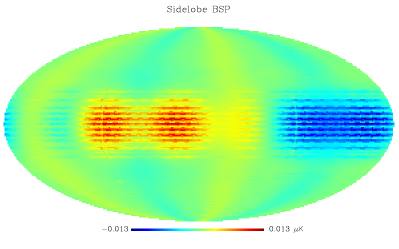
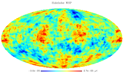
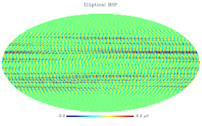
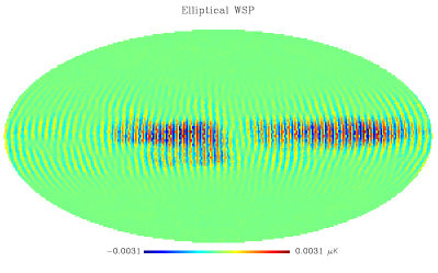
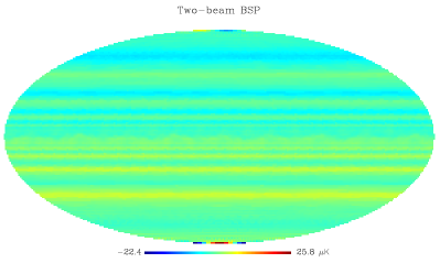
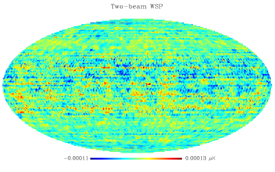
The first beam is a simple model of a sidelobe; it is composed of a Gaussian beam of $\mathrm{FWHM}=1800^{\prime}$ rotated at $90^{\circ}$ to another Gaussian beam of $\mathrm{FWHM}=180^{\prime}$. Both the main beam and the sidelobe are normalized such that they integrate to one. The second beam models a (somewhat exaggerated) elliptical shape, composed of two identical Gaussian beams with $\mathrm{FWHM}=180^{\prime}$ whose centers are on both sides of the optical axis, separated by $180^{\prime}$. The third beam is composed of two identical Gaussian beams ($\mathrm{FWHM}=180^{\prime}$) rotated at $140^{\circ}$ from each other; we refer to this as the two-beam model. This case is motivated by the design of the WMAP observatory BMAP03 .

We set the asymmetry parameter $m_{\rm max}$ for our three cases (sidelobe, elliptical, and two-beam) to 8, 38, and 128, respectively.

Following WG01 , we first considered a basic scan path (BSP) in which the beam scans the full sky on rings of constant longitude with no rotation about its outward axis. To be clear, for the case of the sidelobe beam, the smaller beam follows this ringed-scan while the larger beam remains fixed at the equatorial longitude. Similarly, in the two-beam model, one beam follows the ring-scan while the other rotates in smaller circles $140^{\circ}$ away. The central lobe therefore covers the whole sky, while the offset beam remains within a band of $\pm 50^{\circ}$ centered on the ecliptic plane. The elliptical beam simply follows the ring-scan, and is oriented such that its long axis remains perpendicular to the lines of longitude.

A more realistic observational strategy has a beam that revisits locations on the sky in different orientations. Therefore, we model the one-year WMAP scan path followed by one horn. The WMAP scan strategy also covers the full sky and includes a spin modulation of $0.464$ revolutions per minute and a spin precession of one revolution per hour BMAP03 . We used a scaled-down model of the WMAP scan in which the spin modulation is $0.00232$ revolutions per minute and a step size of about 46 seconds (roughly 562 samples per period). This produces a pattern very similar to the spirograph-type pattern shown in Fig. 4 of BMAP03 . We refer to this as the WMAP-like scan path (WSP). The WSP has about six times as many samples as the BSP. For this strategy, the spirograph pattern is followed by the small beam of the sidelobe, the elliptical beam, and both beams of the two-beam model. In the two-beam case both beams are offset from the spin axis of the satellite, to mimic the WMAP scanning geometry. It is not differential in nature, since both beams have positive weight.

We test each beam (sidelobe, elliptical, and two-beam) with both scanning patterns (BSP and WSP) on a sky without Galactic emission. We refer to these as the six main test cases.

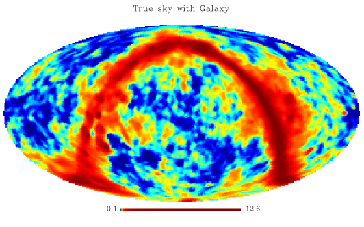
In reality, CMB experiments will also pick up signal from the Galaxy. We use the first-year WMAP Ka-band temperature map, degraded to an $nside$ of 64 and smoothed with a Gaussian beam of $\mathrm{FWHM}=180^{\prime}$ as our model of the true sky with Galactic emission. For our last test case, we convolve it with the sidelobe beam.

For each test case, we assume that the beamshapes of the instrument are known and use the deconvolution method to deconvolve the map with the same beam that the true sky was originally convolved with. We attempt to recover features in the map corresponding to the smallest scale features of our test beams. We therefore set the width of our regularization kernel, represented by the matrix $\mathbf{G}$ in Eqs. (3) and (4), to $\mathrm{FWHM}=180^{\prime}$ in every case. We compare our map estimates to the true sky, smoothed by the regularization kernel. When we refer to the “true” sky in the following we mean this kernel-smoothed input sky.

IV Results and Discussion

We present the results of the deconvolution algorithm for the six main test cases in the form of residual maps. We compare these results to the results from standard map-making by examining their power spectra and by calculating the root mean square (RMS) difference between the estimated and true sky. For the tests that include the Galactic signal we show the actual map estimates.

In Fig. 1 we plot ratios of the power spectra of the residual maps (both standard and deconvolved) and the power spectrum of the input map. The BSP (WSP) results are plotted in the left (right) column. The solid (dashed) lines represent the relative difference in $C_{\ell}$ between the deconvolved (standard) map and true sky map. The standard map-making algorithm failed to give meaningful results for the two-beam test. We therefore excluded this case from the plot.

For all cases we chose to present the results after a fixed number of iterations to show the impact of scanning strategy and beam pattern on the condition number of the map-making equations. We find that the deconvolution algorithm outperforms standard map-making by orders of magnitude in accuracy.

For a fixed number of iterations, the BSP tests performed less well than the WSP tests. The two-beam BSP and, to a lesser extent, the elliptical beam BSP test cases have not converged to sufficient accuracy.

There are several possible causes for this behaviour. The BSP leads to an extremely non-uniform sky coverage. Also, the BSP visits each pixel in a narrow range of beam orientations. Further, the number of sky samples is smaller for the BSP case than for the WSP case (as noted in section III). All of these aspects can contribute to increasing the condition number of the normal equation, which in turn leads to smaller error decay per iteration of the preconditioned CG solver.

Figure 1: Ratios of the spectra of the residual map to the spectrum of the input map for each of the beam models and both scanning strategies. The BSP results are plotted in the left column and the WSP results are plotted in the right column. Results for the sidelobe, elliptical and two-beam beam are shown in the top, middle, and bottom panels, respectively. The solid lines correspond to deconvolved spectra and the dashed lines correspond to the standard spectra.

In Table 1 we summarize the RMS difference between the reconstructed and true sky. The RMS values are computed using the standard deviations the residual and true maps:

$$\mathrm{RMS}=\frac{\mbox{stdev(residual map)}}{\mbox{stdev(true map)}}$$ (14)

where

$$\mbox{residual map}={\mbox{estimated map}-\mbox{true map}}.$$ (15)

The RMS values reflect the trends seen in the spectra in Fig. 1. The residual maps are shown in Fig. 2. In order that the scale of the axes on the residual maps are meaningful, we also show the true sky map.

	BSP		WSP
Beam	Standard	Deconvolved	Standard	Deconvolved
Sidelobe	0.257467	0.000111903	0.178828	3.13741e-07
Elliptical	0.186262	0.0207830	0.129715	2.25602e-05
Two-beam	N/A	0.102778	N/A	1.08579e-06

Table 1: Fractional RMS error for each of the six main test cases.

Figure 2: Residuals after the first 100 iterations are shown in the first three rows. The figures on the left are for the basic scan path the ones on the right for the WMAP-like scan path. First, second, and third rows correspond to the sidelobe, elliptical and two-beam beams, respectively. The true sky is shown in the fourth row. Note that solutions of the two-beam BSP and, to a lesser extent, the elliptical beam BSP test cases have not converged to sufficient accuracy. We chose to present the results for all cases after a fixed number of iterations to show the impact of scanning strategy and beam pattern on the condition number of the map-making equations.

Achieving a stably converging iterative solution method for the deconvolution problem is a success of our regularization technique. The convergence of our iterative solver as function of iteration number is plotted in Fig. 3.

In order to be able to compare the performance of our method for different beam patterns and scanning strategies we make the deliberate choice of limiting the number of iterations to 100 and comparing the best results obtained up to this point. Since our error estimate continues to drop stably (except in two cases, where we reach the single precision numerical accuracy floor after $\sim 25$ and $\sim 70$ iterations) it is clear that the accuracy of the reconstruction can be improved by allowing the system to iterate further, or by choosing a more sophisticated pre-conditioner.

Figure 3: Convergence rates of the preconditioned conjugate gradient solver for each test case. The left panel refers to the basic scan path and the right panel to the WMAP-like scan path. The solid lines correspond to the sidelobe beam, dotted lines to the elliptical beam, and dot-dashed to the two-beam model.

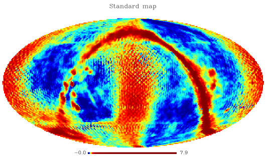
Our final test case consists of a model sky with Galaxy emission convolved with the sidelobe beam over the WSP. We present the output maps of both the standard and deconvolution methods in Fig. 4, where the maps are shown in ecliptic coordinates. One can see that the standard map contains a distorted image of the Galaxy and that the deconvolved map is virtually identical to the true map.

Figure 4: Deconvolving the effects of a large sidelobe in simulated observations of the WMAP Ka band map, using the coarsened WMAP scanning strategy described in the text. The top map is the input sky map, the middle map is the standard map-making result, and the bottom map is the deconvolved result.

V Conclusions and Future Work

We have presented a deconvolution map-making method for data from scanning CMB telescopes. Our methods remove artifacts due to beam asymmetries and far sidelobes. We compare our technique with the standard map-making method and demonstrate that the true sky is recovered with greatly enhanced accuracy via the deconvolution method. Deconvolution map-making recovers features of the CMB sky on the smallest scale of the beam, thereby achieving a form of super-resolution imaging. This extracts more of the information content in CMB data sets.

One of the key difficulties encountered in deconvolution problems is that the systems of linear equations we need to solve are very nearly singular. We solve this problem by introducing a regularization method which allows us to solve the systems stably and recover maps at a uniform resolution and with an effective beam that is azimuthally symmetric and has a Gaussian profile.

We tested the convergence speed of two particular scanning strategies and found that the WMAP-like scan is superior to the basic scan in both rate of convergence and true-sky recovery. We hypothesize that this is due to the nature of the BSP, where the poles are the location of the only beam crossings and receive many more hits than the rest of the sky. In addition, our implementation of the BSP had a smaller number of samples overall than our implementation of the WSP.

We have also shown the relevance of this algorithm to the WMAP mission by demonstrating its operation using a WMAP-like scanning strategy and a two-beam model which, while not differential, resembles the telescope orientations of the WMAP spacecraft. Our results underline the qualities of the WMAP scanning strategy compared to a BSP strategy for deconvolution map-making.

In order to decouple from issues that are not directly related to the optical performance of CMB instruments we did not consider the effects of noise in our simulations. For a realistic assessment of the performance of our methods on real data this needs to be added. In particular, the choice of scale for the regularization kernel will depend on weighing the benefits of increased resolution against increased high-frequency.

Recently several groups have published CMB polarization results on the EE power spectrum polarization . WMAP released an all-sky analysis of the TE cross-correlation in the first year data WMAPpol . We eagerly anticipate the large-angle polarization data from WMAP in the impending release of the second year data. In a few years’ time, polarimeters on board the Planck satellite will collect data. Owing to the difficulty of separating the two polarization modes, we expect that polarimetry experiments will be very sensitive to beam asymmetries and stray light. Future measurements of the tiny B-mode polarization will require both exquisite instruments and sophisticated analysis tools. We hope that the generalization of our methods to polarized map-making will be useful for making maps of the polarized microwave sky. It has already been shown C00 that little modification to the Wandelt-Górski method of fast all-sky convolution is needed to accomodate polarization data.