The interstellar C¹⁸O/C¹⁷O ratio in the solar neighbourhood: The $\rho$ Oph cloud

Abstract

Observations of up to ten carbon monoxide (CO and isotopomers) transitions are presented to study the interstellar C¹⁸O/C¹⁷O ratio towards 21 positions in the nearby ($d$$\sim$140 pc) low-mass star forming cloud $\rho$ Oph. A map of the C¹⁸O $J$=1–0 distribution of parts of the cloud is also shown. An average ¹²C¹⁸O/¹²C¹⁷O isotopomeric ratio of 4.11 $\pm$ 0.14, reflecting the ¹⁸O/¹⁷O isotope ratio, is derived from Large Velocity Gradient (LVG) calculations. From LTE column densities we derive a ratio of 4.17$\pm$0.26. These calculations also show that the kinetic temperature decreases from about 30 K in the cloud envelope to about 10 K in the cloud cores. This decrease is accompanied by an increase of the average molecular hydrogen density from 10⁴ cm^-3 to $\ga$10⁵ cm^-3. Towards some lines of sight C¹⁸O optical depths reach values of order unity.

1 Introduction

Abundance ratios of interstellar isotopomers are a powerful tool to study the chemical evolution of the Galaxy. One such ratio is that of the rare species of oxygen, ¹⁸O and ¹⁷O, as measured from the isotopomers of CO. For the galactic disk and -center region, Penzias ([1981]) reported average ¹⁸O/¹⁷O ratios of 3.65$\pm$0.15 and 3.5$\pm$0.2, respectively. He also found that the ¹⁸O/¹⁷O ratio, determined from the integrated line intensity ratios $\int$T[¹²C¹⁸O(1$-$0)]d$v$/$\int$T[¹²C¹⁷O(1$-$0)]d$v$, shows no significant gradient with galactocentric distance $R$ out to 10 kpc (solar circle: $R_{0}$=8.5 kpc): the ¹⁸O/¹⁷O ratios of the galactic disk and -center are, within the limits of observational accuracy, identical. Models of the chemical evolution of the Galaxy by Prantzos et al. ([1996]) suggest that after a few Gyr the ratios in the Galaxy should be independent of galactocentric radius. There is, however, a discrepancy between the interstellar medium (ISM) values and the much higher (5.5; Anders & Grevesse [1989]) solar system one. Heikkilä et al. ([1998]) obtain a low value of 1.6$\pm$0.3 in the LMC, while in the nuclear starbursts NGC 253 and NGC 494 5 ¹⁸O/¹⁷O $\sim$ 6.5 (Harrison et al. [1999]; Wang et al. [2004]). These results suggest that the ¹⁸O/¹⁷O ratio depends on metallicity.

The sources observed by Penzias are located in a limited range of galactocentric radius (and therefore metal abundance), and we (Wouterloot et al., in preparation) have reobserved these sources with higher angular resolution and have extended our study to sources out to $R$=16 kpc. While Penzias ([1981]) only observed the $J$=1–0 transition, our observations also include the $J$=2–1 rotational lines. The goal of the present paper is to study in detail excitation and opacity effects that could affect the measured ¹⁸O/¹⁷O ratios and radial gradients on small scales. These effects are usually either ignored or physical parameters are derived by assuming a fixed ¹⁸O/¹⁷O ratio, so that a more careful study is desirable.

We have chosen the $\rho$ Oph cloud ($d$$\sim$140 pc) because of the large range in column densities found therein, and because it is in the solar neighbourhood so that a high linear resolution can be attained towards this object. Twenty one positions were selected for observations from a C¹⁸O(1–0) map of Wilking & Lada ([1983]) to have a range of C¹⁸O(1–0) intensities. Towards the positions with the strongest lines we not only observed the $J$=1–0 and 2–1 lines of four isotopomers (¹²C¹⁶O, hereafter ¹²CO; ¹³C¹⁶O, hereafter ¹³CO; ¹²C¹⁸O, hereafter C¹⁸O; ¹²C¹⁷O, hereafter C¹⁷O), but we also measured the $J$=3–2 lines of C¹⁸O and C¹⁷O.

2 Observations

2.1 SEST observations

Between September 19 and October 5, 1987 we used the 15-m Swedish-ESO Submillimeter Telescope (SEST) to map C¹⁸O(1–0) towards a part of the $\rho$ Oph cloud. We employed a Schottky receiver in combination with an acousto-optical spectrometer (AOS) which had a channel separation of about 43 kHz (0.12 km s^-1). All observations were made using frequency switching. The spectra were folded and subsequently resampled to a channel width of 0.24 km s^-1. The rms of the resampled data is typically 0.14 K ($T_{\rm A}^{*}$). A 15$\times$ 15 region was observed with a 40 (in part of the map 20) raster (the beam size of the SEST at 110 GHz is about 47). The mapped region contains the cloud cores $\rho$Oph B1, $\rho$Oph C, $\rho$Oph E, and $\rho$Oph F, as defined from DCO⁺ maps by Loren et al. ([1990]).

Between January 26 and 31, 1999 we used two SIS receivers at the SEST to observe ¹²CO, ¹³CO, C¹⁸O, and C¹⁷O $J$=1–0 and 2–1 towards 21 positions in the $\rho$ Oph cloud. The observed transitions and frequencies are given in Cols. 1 and 2 of Table 1. Col. 3 gives the beam size and Cols. 4 and 5 the main beam- and moon efficiencies of the telescope used (Col. 6). Most intensities in this paper are on the $T_{\rm A}^{*}$ scale because then uncertain corrections to $T_{\rm R}^{*}$ or $T_{\rm{mb}}$ do not affect the discussed ratios. In some places, i.e. when comparing lines from different rotational transitions, the use of a different scale (main beam brightness temperature, $T_{\rm{mb}}$, or the average of $T_{\rm{A}}^{*}$ and $T_{\rm{mb}}$) was unavoidable. This is then mentioned explicitly. The pointing accuracy was about 5.

The observed positions were selected from the C¹⁸O map of Wilking & Lada ([1983]), and span a large range in C¹⁸O intensity and hence in $A_{v}$; they are listed in Table 2, in order of decreasing intensity (as estimated from the Wilking & Lada map). Given are a reference number in Col. 1; the position in equatorial coordinates in Cols. 2 and 3; the offset positions with respect to $\alpha$(1950)=16^h24^m10^s, $\delta$(1950)=$-$2423 (this is the average of the H₂CO (Martin-Pintado et al. [1983]) and NH₃ (Zeng et al. [1984]) positions determined for core B1 with the 100-m telescope at Effelsberg)[$\alpha$(2000)=16^h27^m11.6^s, $\delta$(2000)=$-$242942], and the rms in the observed transitions in Cols. 6 to 15.

Towards all positions (1 to 21) we observed each of the four isotopomers simultaneously in the $J$=1–0 and 2–1 transitions. The observations were made using frequency switching and we used the high resolution spectrometer (AOS channel-spacing about 43 kHz) split into two equal parts. Integration times were chosen to obtain similar signal to noise ratios in the C¹⁷O and C¹⁸O spectra in order to accurately derive the line ratios. In addition to the single positions we made small (3$\times$3) maps centered on the selected 21 positions on a 20 raster in C¹⁸O ($J$=2–1) to see whether the positions are located in regions with large gradients where pointing errors can influence the observed line ratios, and to be able to convolve the $J$=2–1 data to the $J$=1–0 angular resolution.

Figure 1: Distribution of C¹⁸O(1–0) emission towards the $\rho$ Oph cloud. a. Integrated between $-$1 and +8 km s^-1. Contour levels are 2 to 10 K km s^-1 in steps of 1 K km s^-1. Small crosses indicate the observed positions. Offsets are with respect to $\alpha$(1950)=16^h24^m10^s, $\delta$(1950)=$-$2423. The filled circles are those of the 21 positions (see Table 2) that were also observed in other isotopomers and that are located within or very near the mapped region. b. Peak $T_{\rm A}^{*}$ in the same velocity interval. Contour levels are 0.5 to 4.5 K in steps of 0.5 K. The open circle indicates the angular resolution of the SEST. The crosses indicate in order of decreasing declination the DCO⁺ cores B1, C, E, and F (Loren et al. [1990]).

2.2 JCMT observations

On July 14, 2001, we observed C¹⁷O(3–2) towards eight of the 21 positions with the 15-m James Clerk Maxwell Telescope (JCMT) using frequency switching. The velocity resolution of the autocorrelation spectrometer was 0.14 km s^-1 and the rms noise level ranged from 0.07 to 0.14 K, depending on the line intensity (we tried to reach similar signal-to-noise ratios at all positions).

On February 28, 2002 we observed in the same way C¹⁸O(3–2) towards six of the positions previously observed in C¹⁷O(3–2). The rms listed in Cols. 8 and 11 of Table 2 was 0.14 to 0.33 K.

Table 1: Observed transitions

Molecule	Frequency	Beam	$\eta$mb	$\eta$moon	Tel.
	(MHz)
${}^{12}{\rm C}^{18}{\rm O}$(1$-$0)	109782.160	47	0.7	0.9	SEST
${}^{13}{\rm C}^{16}{\rm O}$(1$-$0)	110201.353	47	0.7	0.9	SEST
${}^{12}{\rm C}^{17}{\rm O}$(1$-$0)	112358.988	46	0.7	0.9	SEST
${}^{12}{\rm C}^{16}{\rm O}$(1$-$0)	115271.204	45	0.7	0.9	SEST
${}^{12}{\rm C}^{18}{\rm O}$(2$-$1)	219560.319	24	0.5	0.9	SEST
${}^{13}{\rm C}^{16}{\rm O}$(2$-$1)	220398.686	24	0.5	0.9	SEST
${}^{12}{\rm C}^{17}{\rm O}$(2$-$1)	224714.368	24	0.5	0.9	SEST
${}^{12}{\rm C}^{16}{\rm O}$(2$-$1)	230537.990	23	0.5	0.9	SEST
${}^{12}{\rm C}^{18}{\rm O}$(3$-$2)	329330.545	14	0.6	0.9	JCMT
${}^{12}{\rm C}^{17}{\rm O}$(3$-$2)	337061.130	14	0.6	0.9	JCMT

Table 2: Observed sources and rms values (K on a $T_{\rm A}^{*}$ scale) for individual transitions.

Pos.	$\alpha$(1950)	$\delta$(1950)	Offseta		rms C17O			rms C18O			rms 13CO		rms 12CO
	h m s				1–0	2–1	3–2	1–0	2–1	3–2	1–0	2–1	1–0	2–1
1	16 23 54.0	-24 27 45	-3.55	-4.75	0.023	0.029	0.085	0.050	0.070	0.14	0.12	0.20	0.20	0.23
2	16 23 11.6	-24 14 20	-13.20	8.27	0.025	0.042	0.140	0.068	0.091	0.21	0.07	0.14	0.27	0.26
3	16 24 02.1	-24 31 33	-0.53	-8.55	0.018	0.032	0.071	0.070	0.066	0.19	0.15	0.20	0.30	0.30
4	16 24 02.7	-24 29 41	-1.67	-6.68	0.019	0.025	0.081	0.053	0.078	0.20	0.15	0.22	0.27	0.26
5	16 23 28.6	-24 16 34	-9.43	6.60	0.017	0.031	0.076	0.052	0.077	0.33	0.13	0.20	0.30	0.30
6	16 24 13.4	-24 33 32	0.77	-10.53	0.026	0.028	0.086	0.060	0.087	0.28	0.17	0.20	0.30	0.33
7	16 23 31.9	-24 20 00	-8.68	3.00	0.016	0.029	0.145	0.058	0.077		0.14	0.21	0.34	0.30
8	16 24 18.1	-24 30 21	1.85	-7.35	0.013	0.020	0.103	0.045	0.051		0.12	0.19	0.35	0.33
9	16 23 11.2	-24 13 30	-13.38	9.50	0.020	0.029		0.072	0.074		0.12	0.20	0.34	0.30
10	16 23 48.0	-24 22 11	-5.02	0.82	0.019	0.031		0.104	0.063		0.14	0.19	0.39	0.34
11	16 24 26.0	-24 27 28	3.65	-4.47	0.023	0.033		0.079	0.059		0.15	0.18	0.33	0.28
12	16 23 33.8	-24 10 48	-8.25	12.20	0.018	0.025		0.071	0.059		0.14	0.22	0.36	0.33
13	16 23 35.5	-24 25 23	-7.85	-2.38	0.012	0.020		0.067	0.060		0.13	0.24	0.38	0.33
14	16 23 50.0	-24 18 20	-4.55	4.67	0.016	0.026		0.071	0.049		0.16	0.20	0.39	0.36
15	16 23 18.3	-24 18 14	-11.77	4.77	0.012	0.017		0.076	0.051		0.16	0.23	0.36	0.34
16	16 23 20.5	-24 23 06	-11.27	-0.10	0.0072	0.014		0.031	0.030		0.15	0.21	0.38	0.35
17	16 24 20.9	-24 15 23	2.48	7.62	0.011	0.016		0.057	0.042		0.13	0.22	0.33	0.34
18	16 23 12.8	-24 09 16	-13.02	13.73	0.011	0.012		0.051	0.041		0.13	0.22	0.32	0.28
19	16 23 05.8	-24 23 06	-14.62	-0.10	0.010	0.019		0.038	0.032		0.16	0.21	0.35	0.32
20	16 24 33.4	-24 15 23	5.33	7.62	0.0066	0.010		0.034	0.037		0.13	0.19	0.32	0.38
21	16 23 25.6	-24 07 07	-10.12	15.88	0.010	0.017		0.042	0.050		0.14	0.23	0.28	0.30
a. With respect to $\alpha$(1950)=16h24m10s, $\delta$(1950)=$-$2423

3 Results

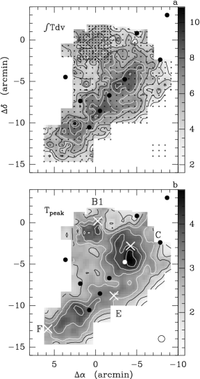
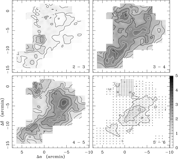
The C¹⁸O(1–0) distribution in the mapped region is shown in Fig. 1. The map includes the cloud cores $\rho$Oph B1, $\rho$Oph C, $\rho$Oph E, and $\rho$Oph F (see e.g. the 1.3 mm continuum map in Fig. 1 of Motte et al. ([1998]) which indicates the locations of the cores A, B1, B2, C, D, E, and F). These cores were originally defined in DCO⁺ maps by Loren et al. ([1990]). We show the emission integrated over all velocities (–1 to 8 km s^-1) in Fig. 1a and the peak $T_{\rm A}^{*}$ distribution in Fig. 1b, respectively. A comparison between the panels (and Gaussian fits to the lines) shows that $\rho$Oph B1 and $\rho$Oph C (near offsets (0, 0) and (–4,–3) respectively) have relatively narrow lines (about 1.5 km s^-1) and a (more) pronounced peak in Fig. 1b, whereas broader (about 2.3 km s^-1) lines occur north of $\rho$Oph E, near ($-1,-8$). At the edges of the map, near $\rho$Oph F, southwest of $\rho$Oph C, and in between $\rho$Oph B1 and $\rho$Oph C line widths reach values of about 1.0 km s^-1. Compared to the lower angular resolution C¹⁸O(1–0) map in Fig. 2 of Wilking & Lada ([1983]; beam size 1.1 on a 1 or 2 raster), the distribution in Fig. 1 shows finer spatial structure. There is also a reasonable correlation between the 1.3 mm continuum in Fig. 1 of Motte et al. ([1998]) and the C¹⁸O distribution. The C¹⁸O $J$=1–0 emission in four 1 km s^-1-wide channels is shown in Fig. 2. $\rho$Oph C and $\rho$Oph E are mainly observed at 4$-$5 km s^-1, whereas $\rho$Oph B1 and $\rho$Oph F show most emission at 3$-$4 km s^-1.

Figure 2: C¹⁸O(1–0) distribution in four velocity intervals (given in the lower right hand corner of each panel). Contour levels are 0.5 to 4.5 K km s^-1 in steps of 0.5 K km s^-1.

All spectra measured towards the first three of the twenty-one positions (Table 2) are shown in Fig. 3 (the spectra towards all positions are published in the Appendix in the electronic edition). The velocity interval is $-$8 to +16 km s^-1. Most ¹²CO and some ¹³CO spectra show self-absorption (a clear minimum in between two peaks in the spectra that is not seen in the lines of the rarer CO isotopomers). If flat-topped spectra are also considered as an indication for self-absorption, this phenomenon occurs at even more positions. The numbers in the boxes of the C¹⁸O(2–1) profiles show the values of $\int$$T_{\rm A}^{*}$[C¹⁸O(2–1)]d$v$ for the 20-spaced nine-point map around each position. Some positions show significant (10 to 15%) intensity gradients where pointing differences between C¹⁸O and C¹⁷O (which were not observed simultaneously) could influence the derived line ratios. Equivalent line widths ($\int$$T_{\rm A}^{*}$d$v$/1.06$T_{\rm A}^{*}$[peak]) for C¹⁸O(1–0) range between 0.84 km s^-1 (pos. 14) and 1.91 km s^-1 (pos. 8). At many positions the C¹⁸O and C¹⁷O line profiles show the presence of several velocity components, which are more pronounced in ¹³CO and ¹²CO (but at slightly different velocities, probably due to self-absorption and saturation in the more abundant isotopomers). Two of these velocity components are visible (at 3–4 and 4–5 km s^-1) in the C¹⁸O(1–0) channel maps of Fig. 2. The C¹⁷O spectra also show hyperfine structure (see e.g. Lovas & Krupenie [1974]).

Figure 3: ¹²CO, ¹³CO, C¹⁸O and C¹⁷O spectra towards the first three of the selected positions given in Table 2. Numbers in the C¹⁸O(2–1) panels indicate integrated line intensities in K km s^-1 on a 20 raster centered at the respective position. The complete set of spectra can be obtained in FITS format at http://cdsweb.u-strasbg.fr/cgi-bin/qcat?J/A+A/

Table 3: Observed C¹⁷O, C¹⁸O, and ¹³CO (1–0), (2–1), and (3–2) integrated line intensities and line ratios (i.e. not corrected for the frequency difference). For each position the second line gives the formal errors not including calibration uncertainties.

Pos.	C17O			C18O			13CO		${\rm{C^{18}O}}\over{\rm{C^{17}O}}$	${\rm{C^{18}O}}\over{\rm{C^{17}O}}$	${\rm{C^{18}O}}\over{\rm{C^{17}O}}$	${\rm{{}^{13}CO}}\over{\rm{C^{18}O}}$	${\rm{{}^{13}CO}}\over{\rm{C^{18}O}}$
	(1–0)	(2–1)	(3–2)	(1–0)	(2–1)	(3–2)	(1–0)	(2–1)	(1–0)	(2–1)	(3–2)	(1–0)	(2–1)
	K km s-1
1	4.12	3.79	2.03	8.59	6.60	4.06	24.45	15.46	2.08	1.74	2.00	2.85	2.34
	0.02	0.02	0.10	0.05	0.05	0.16	0.12	0.15	0.02	0.02	0.12	0.02	0.03
2	2.25	3.52	3.52	6.82	10.07	8.42	43.07	35.38	3.03	2.86	2.39	6.31	3.51
	0.03	0.03	0.16	0.07	0.07	0.24	0.08	0.10	0.05	0.03	0.13	0.07	0.03
3	2.50	2.43	1.22	8.33	7.17	3.13	27.03	19.12	3.33	2.95	2.57	3.24	2.66
	0.02	0.02	0.08	0.07	0.05	0.22	0.15	0.15	0.04	0.03	0.25	0.03	0.03
4	2.62	2.29	1.49	7.52	6.62	3.65	25.33	18.31	2.87	2.89	2.45	3.37	2.77
	0.02	0.02	0.09	0.05	0.06	0.23	0.16	0.16	0.03	0.03	0.22	0.03	0.03
5	1.27	2.69	3.38	4.27	6.74	8.48	34.31	28.68	3.36	2.50	2.51	8.03	4.26
	0.02	0.02	0.09	0.05	0.06	0.38	0.14	0.15	0.06	0.03	0.13	0.11	0.04
6	2.00	2.06	0.95	7.02	6.00	3.21	22.31	16.41	3.51	2.91	3.37	3.18	2.73
	0.03	0.02	0.10	0.06	0.06	0.33	0.18	0.15	0.06	0.04	0.49	0.04	0.04
7	1.97	3.71	4.85	6.31	8.84		33.63	23.46	3.20	2.38		5.33	2.65
	0.02	0.02	0.17	0.06	0.06		0.14	0.15	0.04	0.02		0.06	0.02
8	1.47	1.37	0.57	5.20	4.84		24.02	15.08	3.55	3.53		4.61	3.12
	0.01	0.01	0.12	0.05	0.04		0.13	0.14	0.05	0.05		0.05	0.04
9	2.04	3.44		7.79	10.85		40.61	29.41	3.82	3.15		5.21	2.71
	0.02	0.02		0.08	0.05		0.12	0.15	0.05	0.02		0.05	0.02
10	1.41	1.63		2.97	4.27		21.81	14.73	2.10	2.62		7.35	3.45
	0.02	0.02		0.11	0.05		0.14	0.14	0.08	0.05		0.27	0.05
11	1.25	1.17		4.53	3.80		20.52	13.59	3.62	3.24		4.53	3.58
	0.02	0.02		0.08	0.04		0.15	0.13	0.09	0.08		0.09	0.05
12	1.20	2.36		4.32	5.47		24.53	16.41	3.60	2.32		5.69	3.00
	0.02	0.02		0.07	0.04		0.14	0.16	0.08	0.03		0.10	0.04
13	0.83	1.38		2.40	3.47		25.52	16.69	2.88	2.52		10.63	4.80
	0.01	0.01		0.07	0.04		0.13	0.18	0.09	0.04		0.31	0.08
14	0.95	1.35		2.87	3.30		16.25	14.59	3.00	2.45		5.66	4.43
	0.02	0.02		0.07	0.04		0.17	0.15	0.09	0.04		0.16	0.07
15	1.07	2.06		3.71	6.40		37.64	33.15	3.47	3.11		10.14	5.18
	0.01	0.01		0.08	0.04		0.17	0.17	0.08	0.03		0.22	0.04
16	0.33	0.59		1.11	1.69		19.45	15.78	3.36	2.86		17.55	9.35
	0.01	0.01		0.03	0.02		0.16	0.15	0.12	0.06		0.53	0.15
17	0.65	0.67		2.36	2.56		16.94	11.33	3.65	3.80		7.17	4.43
	0.01	0.01		0.06	0.03		0.13	0.16	0.11	0.08		0.19	0.08
18	0.55	1.05		1.94	3.32		24.13	17.47	3.55	3.15		12.46	5.27
	0.01	0.01		0.05	0.03		0.13	0.16	0.12	0.04		0.35	0.07
19	0.32	0.67		0.98	1.62		18.85	15.80	3.08	2.43		19.20	9.77
	0.01	0.01		0.04	0.02		0.16	0.15	0.16	0.06		0.80	0.17
20	0.37	0.44		1.56	1.78		17.10	11.87	4.20	4.07		10.95	6.65
	0.01	0.01		0.03	0.03		0.14	0.14	0.12	0.09		0.26	0.13
21	0.40	0.88		1.67	2.29		17.92	12.85	4.16	2.61		10.71	5.61
	0.01	0.01		0.04	0.04		0.15	0.17	0.15	0.06		0.30	0.12

4 Isotopomeric ratios

4.1 Isotopomeric ratios derived from line intensities

Integrated line intensities over the velocity interval $-$1.5 to 8 km s^-1 (i.e. over all velocity components) and their ratios at the measured 21 positions are listed in Table 3 for C¹⁷O, C¹⁸O, and ¹³CO. For each position the first line gives the intensities (Cols. 2 to 9) and ratios (Cols. 10 to 14) and the second line the uncertainty therein, obtained from the rms in the baseline. We note that while we obtained the positions from the C¹⁸O(1–0) map of Wilking & Lada ([1983]) and ordered them according to an expected decrease in integrated intensity, we see this in our results, but there is significant scatter. This is likely caused by a lower angular resolution and undersampling in the Wilking & Lada map, compared to our data. The selected positions cover a large range in C¹⁸O(1–0) integrated intensity (from 0.98 to 8.59 K km s^-1) (or $A_{\rm v}$ $\approx$ 10 to 200 mag (using column densities in Table 4 and Frerking et al. [1982])), as intended.

The resulting C¹⁸O/C¹⁷O and ¹³CO/C¹⁸O integrated line intensity ratios for the (1–0) and (2–1) transitions as a function of $\int$$T_{\rm A}^{*}$[C¹⁷O(1–0)]d$v$ (the most optically thin transition) are shown in Figs. 4a-d. Here (not in Table 3, following Penzias [1981]) we corrected the ratios for the difference in frequency, which amounts for C¹⁸O/C¹⁷O to a factor 1.047 (C¹⁸O/C¹⁷O(corrected) = ($\nu_{17}/\nu_{18})^{2}$ C¹⁸O/C¹⁷O(observed), see Linke et al. [1977]), but not for optical depth and excitation effects. Therefore, if these effects are negligible, the corrected ratios should be equivalent to those of the column densities. Formal errors derived from the uncertainties in the line areas (see Table 3) are small with respect to the errors introduced by the calibration uncertainties. The latter may amount to 7% causing an error in the ratios of 10%. The 3$\times$3 C¹⁸O(2–1) maps around the observed positions (see Fig. 3) show that over an angular scale of 20 the change in integrated intensity is typically 10% or less. This implies that pointing errors of 5 cause errors of a few percent in the observed line intensity ratios. In Fig. 4b we also show (as filled circles) the C¹⁸O/C¹⁷O ratios derived from the JCMT $J$=3–2 observations. These agree well with the $J$=2–1 and $J$=1–0 results. For comparison we also show in Fig. 4a the average result from Penzias ([1981]) for the galactic disk as a dashed line, and the value towards our pos. 1 derived by Bensch et al. ([2001]) from ¹³C¹⁸O and ¹³C¹⁷O(1–0) observations as a dotted line.

At pos. 1, where integrated C¹⁷O line intensities and CO column densities are highest, the observed C¹⁸O/C¹⁷O ratios are significantly lower than towards the other positions (see Figs. 4a,b). This holds for all three observed rotational transitions. At pos. 10 the C¹⁸O/C¹⁷O ratio is lower than at other positions (except pos. 1) for $J$=1–0 but not for $J$=2–1. Omitting pos. 1, the unweighted average of the C¹⁸O/C¹⁷O integrated intensity ratios (including frequency correction) is 3.53$\pm$0.48 (sd; me 0.11) for the (1–0) and 3.06$\pm$0.49 (sd; me 0.11) for the (2–1) transition (for average values we derive both the standard deviation (sd) and the error in the mean (me=sd/$\sqrt{N}$), which is the most relevant parameter describing the uncertainty of the average values). For $J$=3–2 (positions 2 to 6) we obtain a ratio of 2.78$\pm$0.40 (sd; me 0.18); for the same positions the $J$=1–0 and 2–1 ratios are 3.37$\pm$0.26 (sd; me 0.12) and 2.95$\pm$0.18 (sd; me 0.08), respectively, suggesting a decrease of the ratio with $J$, possibly because of increasing optical depth (see Sect. 4.2.3). At pos. 1 the ratios are 2.18$\pm$0.02 (1–0), 1.82$\pm$0.02 (2–1), and 2.09$\pm$0.12 (3–2).

In Figs. 4c,d ¹³CO/C¹⁸O ratios are shown for the (1–0) and (2–1) transitions. This ratio may be strongly affected by ¹³C fractionation for small column densities (Bally & Langer [1982], Langer et al. [1984]), self-shielding (van Dishoeck & Black [1988]), and by high ¹³CO optical depths at large column densities, which explains the decrease from 10 to 20 in the outer parts of the $\rho$ Oph cloud to about 3 in the cloud centre. This decline in integrated line intensity ratios is similar to that seen in Barnard 5 (Langer et al. ([1989]), their Fig. 5), but in $\rho$ Oph ¹³CO/C¹⁸O ratios reach even lower values than in Barnard 5. Towards the very outer parts of Barnard 5 where $\int$T[¹³CO(1–0)]d$v$ is 1-4 K km s^-1, this ratio also decreases. In $\rho$ Oph we do not see this effect, possibly because here the ¹³CO emission is much stronger towards all observed positions. We note that Zielinsky et al. ([2000]) could explain increasing ¹³CO/C¹⁸O ratios towards the edge of a Photon Dominated Region (PDR) by the presence of few big clumps in the cloud center and many small clumps at the cloud edge.

Figure 4: C¹⁸O/C¹⁷O and ¹³CO/C¹⁸O isotopomeric ratios as a function of $\int$$T_{\rm A}^{*}$[C¹⁷O(1–0)]d$v$ for (a,c) $J$=1–0, (b,d) $J$=2–1 (crosses) and (b) $J$=3–2 (filled circles). The C¹⁸O/C¹⁷O and ¹³CO/C¹⁸O line area ratios have been corrected for the frequency difference (see Sect. 4.1). The dashed line indicates the ratio found by Penzias ([1981]) for the galactic disk, and the dotted line denotes the result from Bensch et al. ([2001]) from ¹³C¹⁸O and ¹³C¹⁷O(1–0).

4.2 Isotopomeric ratios derived from LTE column densities

The isotopomeric ratios are likely to be affected by optical depth effects, which will be strong for CO (most positions show self-absorption), significant for ¹³CO, and not negligible for C¹⁸O. For C¹⁷O small optical depths are expected towards all observed lines of sight. At pos. 1, which shows the highest C¹⁷O column density, the observed integrated intensity ratios for $J$=1–0 C¹⁸O/¹³C¹⁸O and C¹⁷O/¹³C¹⁷O are 35.8 and 68.7, respectively (Bensch et al. [2001]), indicating (assuming that the ¹²C/¹³C ratio is about 70; Wilson & Rood [1994]) that the C¹⁸O optical depth is about 1.5 whereas the C¹⁷O optical depth is small.

Trying to account for optical depth effects, we have derived Local Thermodynamical Equilibrium (LTE) column densities of ¹³CO, C¹⁸O, and C¹⁷O. Below we describe how we calculate excitation temperatures and optical depths.

4.2.1 Excitation temperature

For the calculation of $T_{\rm{ex}}$, both the $T_{\rm A}^{*}$ and the $T_{\rm mb}^{*}$ temperatures scales are relevant. The $T_{\rm mb}$-scale is strictly valid in the extreme case of a source only covering the main beam, while the $T_{\rm A}^{*}$-value applies to the opposite extreme, a very extended source. We have estimated the CO excitation temperatures in two different ways, in each of which we used both $T_{\rm A}^{*}$ and $T_{\rm mb}^{*}$.

Firstly, we derive excitation temperatures from the peak temperatures of CO(1–0) and CO(2–1) using

$$T_{\rm{ex}}=5.532\,\left[\ln\left(1+{5.532\over(T_{10}+0.819)}\right)\right]^{-1},$$

where $T_{10}$ is the peak $T$[¹²CO(1–0)] temperature, or

$$T_{\rm{ex}}=11.064\,\left[\ln\left(1+{11.064\over(T_{21}+0.187)}\right)\right]^{-1},$$

where $T_{21}$ is the peak $T$[¹²CO(2–1)] temperature (method 1). This could underestimate the excitation temperature whenever there is self-absorption. The method helps to constrain excitation temperatures, in particular for the outer parts of the cloud.

Secondly we obtain excitation temperatures from the (2–1)/(1–0) ratio of the integrated intensities of C¹⁸O and C¹⁷O, respectively (method 2), assuming that the transitions are optically thin (if this is not the case (mainly for C¹⁸O) the excitation temperature will be underestimated) and that beam filling effects do not affect the ratio [C¹⁷O: (2–1)/(1–0) = 4.0 exp(–10.78/$T_{\rm{ex}}$); C¹⁸O: (2–1)/(1–0) = 4.0 exp($-$10.54/$T_{\rm{ex}}$)]. The $J$=2–1 C¹⁸O and C¹⁷O data were convolved to the $J$=1–0 resolution using the nine point C¹⁸O $J$=2–1 maps described in Sect. 2 (see also Fig. 3). The corrections are small ($\leq$5% at most positions, but 16% at pos. 19). In contrast to method 1 that uses optically thick CO lines potentially tracing predominantly cloud envelopes, method 2 is based on tracers that are more representative of the entire molecular column density. A comparison of excitation temperatures derived by methods 1 and 2 can show whether there are temperature gradients in the cloud.

Figs. 5a, b show the (2–1)/(1–0) $\int$$T_{\rm A}^{*}$d$v$ ratios for C¹⁸O and C¹⁷O, respectively, as a function of $\int$$T_{\rm A}^{*}$[C¹⁷O(1–0)]d$v$. There is no correlation. In Figs. 5c-f we compare $T_{\rm{ex}}$ derived from $J$=1–0 (Figs. 5c,e) and $J$=2–1 (Figs. 5d,f) ¹²CO $T_{\rm{A}}^{*}$ (Figs. 5c,d) values (this, method 1, should provide upper limits to $T_{\rm{ex}}$) with the excitation temperatures of C¹⁸O and C¹⁷O, derived from the $\int$$T_{\rm A}^{*}$d$v$ (2–1)/(1–0) ratios (method 2). We also show in Figs. 5e,f the excitation temperatures after converting to $T_{\rm{mb}}$ using the efficiencies in Table 1 ($T_{\rm{mb}}$=$T_{\rm A}^{*}$$\eta_{moon}$/$\eta_{mb}$). The values derived from $T_{\rm A}^{*}$[¹²CO] range from 14.1 K ($J$=1–0) and 13.0 K ($J$=2–1) at pos. 3 to 32.7 K (1–0) and 30.9 K (2–1) at pos. 5. These values are for a $T_{\rm A}^{*}$ temperature scale. They are even higher for a $T_{\rm mb}^{*}$ scale: the maximum value is 41 K at pos. 5.

Excitation temperatures derived from C¹⁸O and C¹⁷O (method 2) are generally lower: 6.3 K (pos. 1) to 14.3 K (pos. 19) (C¹⁸O) and 7.2 K (pos. 1) to 21.6 K (pos. 19) (C¹⁷O). Using main beam brightness temperature ratios, the values become larger: 7.9 - 26.4 K (C¹⁸O) and 9.3 - 66.4 K (C¹⁷O) for the same positions.

The OLS bisector mode was used to derive linear regression coefficients (see Isobe et al. [1990]). There is some correlation between the excitation temperatures derived from ¹²CO and C¹⁸O (the correlation coefficient is 0.70 in Figs. 5c). For C¹⁷O, the correlation is slightly less well defined (the correlation coefficient is 0.66; Fig. 5d). For C¹⁸O the slope is closest to 1 for the $T_{\rm{mb}}$ ratios (0.93$\pm$0.16), while we obtain a slope of 1.97$\pm$0.33 for the $T_{\rm A}^{*}$ ratios. For C¹⁷O this is reversed: for the $T_{\rm A}^{*}$ ratios the slope is 1.08$\pm$0.15 whereas that for the $T_{\rm{mb}}$ values it is 0.34$\pm$0.08. The higher values for ¹²CO compared to those from the C¹⁸O and C¹⁷O (2–1)/(1–0) ratios can be explained by higher kinetic temperatures in the outer parts of the clouds (e.g. Castets et al. [1990]) from which the ¹²CO emission mostly originates.

Because the extent of C¹⁸O and C¹⁷O clumps is most likely larger than the main beam, but small compared to the size of the Moon we are using in Sects. 4.2.2, 4.2.3, and 4.3 the average of both efficiencies. The resulting $T_{\rm{ex}}$ for C¹⁸O and C¹⁷O are compared with each other in Fig. 5g. It shows that $T_{\rm{ex}}$ is well correlated for both isotopomers, but for C¹⁷O it can reach higher values than for C¹⁸O. There is no correlation between optical depth and $T_{\rm{ex}}$, and therefore the lower $T_{\rm{ex}}$ of C¹⁸O cannot be explained by the fact that we did not correct for optically thick $J$=2$-$1 lines.

Figure 5: ( 2–1)/(1–0) $\int$$T_{\rm A}^{*}$d$v$ ratios for C¹⁸O (a) and C¹⁷O (b) as a function of $\int$$T_{\rm A}^{*}$[C¹⁷O(1–0)]d$v$. c,d. $T_{\rm{ex}}$[¹²CO(1–0)] vs $T_{\rm{ex}}$ obtained from the ratio (2–1)/(1–0) for C¹⁸O (c) and C¹⁷O (d) using $T_{\rm A}^{*}$ (crosses) or $T_{\rm mb}$ (squares). e,f. The same as in c,d, but for $T_{\rm{ex}}$[¹²CO(2–1)]. In (g) the $T_{\rm{ex}}$ from C¹⁸O and C¹⁷O (using the average of Moon and main beam efficiencies) are compared. The drawn lines indicate equal values.

4.2.2 Optical depth

C¹⁸O optical depths are often derived from C¹⁸O and C¹⁷O data by assuming a certain intrinsic C¹⁸O/C¹⁷O ratio. However the aim of this paper is to determine this ratio and therefore this method cannot be applied.

We tried to fit the C¹⁷O hyperfine components for several positions with small line widths. The optical depth for the main hyperfine component of the $J$=1–0 transition had values of less than a few tenths in most cases. The fitting is complicated by the presence of more than one velocity component, such as a broader underlying component (e.g. at pos. 10, which is also seen in C¹⁸O), or two narrow components (pos. 3, 4, 7). In some cases we could fit line widths and velocities to the corresponding C¹⁸O(1–0) spectrum and could use those as input values for the fit. Sometimes the fit gave a high optical depth for a weak component, which is not realistic. Limited signal-to-noise ratios prevented better determinations of the optical depth in these components.

We also derived optical depths from the excitation temperatures determined by method 2 using the radiative transfer equation (see e.g. Rohlfs & Wilson [1996], Eq. (14.48)). We find that for excitation temperatures from (2–1)/(1–0) ratios using an average efficiency (as defined in Sect. 4.2.1 and Fig. 5g) the highest total C¹⁷O(1–0) optical depth (i.e. the resulting peak optical depth if all hyperfine components had the same frequency) is $\tau_{\rm tot}$ = 1.09 for pos. 1. This is a little high when considering ¹⁸O/¹⁷O ratios of order 4 (Sect. 5) and the results of Bensch et al. (2001; see Sect. 4.2). It is equivalent to a value for the main hyperfine component of about 0.36. At other positions $\tau_{\rm tot}$ ranges from 0.01 to 0.43. For C¹⁸O(1–0) the optical depth is undeterminable (log of negative number) at pos. 1, 3, 4 and 6 (but see Sect. 4.2). At the other positions it ranges from 0.05 to 2.1.

4.2.3 LTE column density ratios

Using the excitation temperature and optical depth derived above, the column density is calculated from

$$N_{lte}={3h10^{5}1.065\over 8\pi^{3}\mu^{2}}{\tau\Delta v\over J}Qe^{E_{J-1}\over kT_{\rm{ex}}}\left[1-e^{-h\nu/kT_{\rm{ex}}}\right]^{-1}$$

with $\Delta v$ denoting the full width at half maximum intensity of the emission line, where the transition is from level $J$ to level $J-1$; $\nu$ is the observed frequency, $Q$ is the partition function (e.g. Rohlfs & Wilson [1996], Eq. (14.50)), and $\mu$ the electric dipole moment of the molecule.

Assuming that the structure of the cloud is somewhere in between that of a point source and a very extended source, we used here for all following calculations telescope efficiencies which are the average of the main beam and moon efficiency. Based on the results discussed in the previous sections we decided to adopt for C¹⁸O and C¹⁷O excitation temperatures and optical depths derived using the respective (2–1)/(1–0) ratios, and for ¹³CO the commonly adopted excitation temperature from the corresponding ¹²CO transition. In this way we derive two sets of LTE column density ratios for the C¹⁸O/C¹⁷O and ¹³CO/C¹⁸O ratios, one based on the $J$=1–0, the other on the 2–1 data.

The results for the 21 positions are given in Table 4. Col. 1 gives the position, Col. 2 the frequency-corrected C¹⁸O/C¹⁷O ratio, and Col. 3 the derived column density ratio. The C¹⁷O excitation temperature, total optical depth and column density are in Cols. 4 to 6. At each position the first row is for $J$=1–0 and the second row for $J$=2–1. Cols. 7 and 8 give the excitation temperatures for C¹⁸O and ¹²CO(1–0), respectively.

The unweighted average $N$(C¹⁸O)/$N$(C¹⁷O) LTE ratio for the $J$=1–0 transition (see Fig. 6a) is 4.07$\pm$1.32 (sd; me 0.32), a higher value than that determined by Penzias ([1981]), but close to that derived by Bensch et al. ([2001]) from ¹³C¹⁸O and ¹³C¹⁷O. Omitting here the highest highly uncertain value (above 8.0, at pos. 11) (the $\tau$ is close to being undetermined and therefore uncertain), the ratio becomes 3.81 $\pm$ 0.23). At four positions (1,3,4,6) the C¹⁸O optical depth was undetermined, but for two of those positions (3,6) a value could be derived using the C¹⁷O excitation temperatures. However we did not use these data points to derive the average $N$(C¹⁸O)/$N$(C¹⁷O) ratio. Similarly, for the $J$=2–1 transition using the same $T_{\rm{ex}}$ as above, the C¹⁸O optical depths were undetermined at positions 1, 2, 3, 4, 6, 7, 9, and 11, where at positions 1 to 4 also the C¹⁷O $T_{\rm{ex}}$ resulted in undetermined $\tau$’s. Ratios derived for this transition are shown in Fig. 6b - the average value without the above mentioned positions is 4.35$\pm$0.35. Omitting here the highest value (above 8.0, at pos. 8), the ratio becomes 4.00$\pm$0.29.

Figure 6: C¹⁸O/C¹⁷O((a, b) and ¹³CO/C¹⁸O (c, d) isotopomeric ratios as a function of $\int$$T_{\rm A}^{*}$[C¹⁷O(1–0)]d$v$. The ratios were derived from LTE column densities using excitation temperatures derived from the corresponding (2–1)/(1–0) ratios, except for ¹³CO where we used $T_{\rm{ex}}$ derived from ¹²CO. The filled symbols indicate positions where the C¹⁷O excitation temperatures were used for the C¹⁸O column density. The dashed line indicates the ratio found by Penzias ([1981]) for the galactic disk, and the dotted line marks the result from Bensch et al. ([2001]) from ¹³C¹⁸O and ¹³C¹⁷O(1–0).

$N$(¹³CO)/$N$(C¹⁸O) ratios are shown in Fig. 6c,d, which were derived from the $J$=1–0 and 2–1 data, respectively. One can see that after correction for optical depths the decrease in ratios towards the cloud center remains. This can be explained by real changes in the ratios such as fractionation; modelling them is beyond the scope of this paper.

Table 4: Derived parameters using average beam efficiencies.

Pos	ratio		$T_{\rm ex}$	$\tau$	N	$T_{\rm ex}$	$T_{\rm ex}$	ratio	$T_{\rm kin}$	log[n(H2)]	$\chi^{2}$
	C18O/C17O		C17O			C18O	12CO(1–0)
	fcorr	N ratio	K	(tot)	cm-2	K	K	C18O/C17O	K	cm-3
	$J$=1$-$0							LVG
	$J$=2$-$1
1	2.18	-	8.0	1.09	7.2 1015	6.9	22.9	4.5	9.4	5.19	4.5
	1.82	-		1.45	7.4 1015
2	3.17	4.22	13.6	0.19	3.0 1015	12.4	27.3	4.0	17.8	4.89	6.8
	3.00	-		0.43	3.1 1015
3	3.49	-	8.7	0.30	3.1 1015	7.7	15.5	4.25	11.5	4.71	18
	3.09	-		0.47	3.0 1015
4	3.01	-	7.9	0.43	3.4 1015	7.8	19.3	3.75	11.2	4.71	20
	3.03	-		0.51	3.2 1015
5	3.52	3.00	24.8	0.05	2.2 1015	14.5	36.3	3.5	23.2	4.71	11
	2.62	3.76		0.15	2.3 1015
6	3.67	-	8.7	0.28	2.4 1015	7.4	18.3	5.0	10.3	4.77	4.7
	3.05	8.95		0.41	2.4 1015
7	3.35	4.03	16.1	0.12	2.7 1015	10.9	31.5	3.88	15.4	4.80	2.7
	2.49	3.51		0.33	2.9 1015
8	3.72	5.30	8.0	0.19	1.7 1015	7.8	16.6	4.5	10.6	4.47	2.9
	3.70	8.56		0.28	1.6 1015
9	4.00	5.57	13.6	0.14	2.6 1015	10.7	24.9	5.0	14.8	4.83	0.9
	3.30	6.03		0.29	2.7 1015
10	2.20	2.54	10.3	0.26	1.8 1015	12.7	26.1	3.0	12.2	4.59	14
	2.75	2.91		0.38	1.7 1015
11	3.78	8.11	8.2	0.23	1.5 1015	7.4	19.2	5.5	9.1	4.71	0.0
	3.40	9.08		0.36	1.4 1015
12	3.77	3.92	18.4	0.07	1.7 1015	10.3	22.0	4.5	10.3	4.71	14
	2.43	5.88		0.17	1.8 1015
13	3.01	3.12	14.1	0.08	1.1 1015	11.7	23.0	3.25	11.2	4.41	0.7
	2.64	3.38		0.14	1.0 1015
14	3.14	4.04	12.1	0.15	1.2 1015	9.6	23.5	4.25	9.7	4.71	0.2
	2.56	4.96		0.25	1.2 1015
15	3.63	3.51	18.7	0.05	1.6 1015	15.3	25.7	3.88	18.3	4.47	0.5
	3.26	3.98		0.12	1.5 1015
16	3.52	3.21	17.6	0.03	4.6 1014	13.6	24.1	3.5	11.2	4.11	6.1
	2.99	3.23		0.05	4.4 1014
17	3.82	4.57	9.3	0.12	7.4 1014	9.5	19.7	4.63	10.8	4.41	4.3
	3.97	5.16		0.19	7.1 1014
18	3.72	3.49	17.5	0.03	7.6 1014	14.5	21.7	3.75	18.4	4.23	0.5
	3.30	3.77		0.08	7.5 1014
19	3.22	2.36	29.5	0.01	6.1 1014	17.5	31.3	3.0	32.5	3.87	9.6
	2.55	2.30		0.03	6.1 1014
20	4.39	4.75	9.5	0.04	4.0 1014	9.0	19.3	4.5	11.2	3.99	0.2
	4.26	4.91		0.07	3.8 1014
21	4.36	3.38	23.2	0.02	6.6 1014	11.2	19.1	4.25	11.2	4.41	41
	2.74	3.74		0.07	6.5 1014

4.3 Isotopomeric ratios derived from Large Velocity Gradient (LVG) modelling

In order to study the excitation of C¹⁸O and C¹⁷O in more detail, we also made LVG calculations (e.g. Castor [1970]; Scoville & Solomon [1974]). Simulating the observed line intensities, one can estimate column densities, H₂ volume densities and kinetic temperatures. The critical point in our LTE approach (Sect. 4.2) is the assumption of a single excitation temperature for all transitions of a given CO isotopomer. The LVG calculations provide a way to estimate in how far differences in derived column densities are accompanied by changes in excitation temperature. In principle, such changes could provide line intensity ratios that do not directly reflect the ¹⁸O/¹⁷O isotope ratio and an LVG code is a suitable tool to investigate such effects.

We used the collision rates from Flower ([2001]) with an ortho/para H₂ ratio of 3.0. Taking instead a ratio of 0.1 (i.e. almost pure para-H₂) does not significantly alter the results outlined below. Level populations and expected line intensities were calculated for 5 K $<$ $T_{\rm kin}$ $<$ 35 K and 10³ $<$ $n$(H₂) $<$ 10⁶ cm^-3. For C¹⁸O we assumed an average abundance of [C¹⁸O]/[H₂] = 1.7 10^-7, derived by Frerking et al. ([1982]) for positions in the $\rho$ Oph cloud. In the calculations we used intrinsic ratios of C¹⁸O/C¹⁷O between 1.5 and 8.0 in steps of 0.25 or 0.5, and adopted a velocity gradient of 5 km s^-1pc^-1, which is appropriate for the size and line width of the $\rho$ Oph clouds.

Before discussing the results we have to check whether the assumptions used by Frerking et al. ([1982]) to derive C¹⁸O column densities, $N$(C¹⁸O), are the same as used in the present paper. They observed C¹⁸O(1–0) towards twelve positions and detected eight of them with a maximum $T_{\rm A}$ of 1.3 K. The positions were selected to have relatively low column densities in order to be able to derive extinctions ($A_{\rm v}$$<$10 mag, where depletion (see below) is not important). Upper limits to column densities were derived assuming that the C¹⁸O excitation temperature equals $T_{\rm{ex}}$ (¹²CO) and that all levels are populated. To derive a lower limit to column densities Frerking et al. ([1982]) assumed the same excitation temperature, but with only the $J$=0 and 1 levels populated. The latter is clearly not true because we detected $J$=2–1 emission in excess of 1.0 K at positions with $T_{\rm{A}}^{*}$[C¹⁸O(1–0)] $<$ 1.0 K. Then Frerking et al. used the average value of upper and lower limit. Comparing our LTE column densities (Sect. 4.2.3) with values derived using Frerking et al.’s assumptions shows that Frerking et al. underestimate column densities by a factor of 2. Therefore the abundance is too small by that amount.

There is another reason why the assumption of a constant abundance is not necessarily correct. Kramer et al. ([1999]) found indications of CO depletion by a factor of about 3 in the core of IC 5146 at visual extinction $A_{\rm v}$ of about 30 mag. IC 5146 is colder than the $\rho$ Oph cloud and Kramer et al. concluded that C¹⁸O(1–0) and (2–1) are optically thin, which is not the case for all positions in $\rho$ Oph. The depletion starts at visual extinctions of about 10 mag (Bergin et al. [2002]), which would correspond to a $N$(C¹⁸O) of $\approx$2 to 4 10¹⁵ cm^-2 (assuming $N$(H₂)/$A_{\rm v}$ 0.9 10²¹ cm^-2mag^-1; Bohlin et al. [1978]). This is in the lower range of the column densities at the observed positions (see Table 4). However depletion is not expected to affect isotopomeric ratios and we have done some LVG calculations using a C¹⁸O abundance which is a factor of 2 lower than that of Frerking et al. ([1982]). The results differ only marginally from those obtained with an undepleted abundance and are therefore inconclusive: at all positions the derived H₂ densities are approximately a factor of two larger and the kinetic temperatures are slightly smaller. Because the effects of depletion and the underestimation of column densities by Frerking et al. may balance out, we decided to use the Frerking et al. ([1982]) abundances in our calculations.

Towards the 21 positions the observed and predicted values of peak C¹⁸O temperatures (using averages efficiencies, but also $T_{\rm{A}}^{*}$ and $T_{\rm{mb}}$ for some calculations) and the C¹⁸O/C¹⁷O ratios for the $J$=1–0, 2–1 and 3–2 lines were compared and $\chi$² values were calculated using for the temperatures an uncertainty $\sigma$ of 10% and for the ratios of the three observed rotational transitions a $\sigma$ of 0.15, 0.15, and 0.20, respectively. The measured temperatures for the $J$=2–1 and 3–2 transitions were convolved to the $J$=1–0 beam, as described in Sect. 4.2.1. Cols. 9 to 12 of Table 4 give the results of the LVG calculations: C¹⁸O/C¹⁷O ratio, kinetic temperature, molecular hydrogen density and $\chi^{2}$, indicating the relative goodness of the solutions between the different positions. Apparently the scatter in isotope ratio is smaller than that obtained with the LTE approach.

The parameters of minimum $\chi^{2}$ are shown in Fig. 7 (for the assumed C¹⁸O/C¹⁷O ratio) and Fig. 8 (for $T_{\rm kin}$ and log(n(H₂))). In Fig. 8b the influence of the assumed temperature scale is also shown. The minimum $\chi^{2}$ values range between 0 (perfect fit) and more than 40 (bad fit; for pos. 21), and do not show a systematically lower value for either temperature scale. Fig. 8b shows a general decrease in density and an increase in $T_{\rm{kin}}$ with decreasing column density (or $\int$$T_{\rm A}^{*}$[C¹⁷O(1–0)]d$v$). LVG modelling assumes that the density is constant along the line of sight, which is probably not true and some lines of sight may have larger density gradients than others in the C¹⁷O emitting region.

For all positions except of pos. 1, Fig.7 shows a clear minimum for some C¹⁸O/C¹⁷O. Ratios ranges from 3.0 to 5.5 with an average value of 4.11$\pm$0.65 (sd; me 0.14). Giving a higher weight to positions with lower $\chi$² increases the ratio slightly to 4.21. The exception is pos. 1 which has the highest H₂ density, where the $\chi$² does not much increase for higher ratios. We did not use ¹³CO data in these calculations because this isotopomer is too much affected by fractionation which makes it impossible to assume a single fractional abundance. Likewise ¹²CO data show (much) higher excitation temperatures than the derived kinetic temperatures (see also Fig. 5c-f). This, like the increase in $T_{\rm kin}$ with decreasing column density mentioned above is consistent with kinetic temperatures decreasing towards the cloud interiors from about 20-30 K to 10 K.

We have to check what the LVG calculations predict for $T_{\rm{ex}}$, since LTE assumes that they are equal for all levels. Fig. 9 shows results of the LVG calculations for an assumed C¹⁸O/C¹⁷O ratio of 4.0. In Fig. 9a the dotted lines indicate the predicted $T_{\rm{ex}}$($J$=1$-$0) for C¹⁷O. It is equal to $T_{\rm{kin}}$ at high densities, but for about 5 10³ $<$ n(H₂) $<$ 5 10⁴ cm^-3 $T_{\rm{ex}}$ is larger than $T_{\rm{kin}}$, while below 5 10³ cm^-3 this situation is reversed. The dashed and full-drawn lines indicate the difference in $T_{\rm{ex}}$($J$=1$-$0) between C¹⁷O and C¹⁸O. $T_{\rm{ex}}$(C¹⁷O) is larger than $T_{\rm{ex}}$(C¹⁸O), in agreement with the observations (see Fig. 5g). For $T_{\rm{kin}}$ $<$ 20 K the difference is less than 1 K. At low densities $T_{\rm{ex}}$(C¹⁸O) is slightly larger than $T_{\rm{ex}}$(C¹⁷O). In Fig. 9b the dotted lines show the difference in $T_{\rm{ex}}$ between the $J$=2$-$1 and $J$=1$-$0 transitions of C¹⁷O. It is small for large n(H₂) or low $T_{\rm{kin}}$, but can reach values of more than 10 K for $T_{\rm{kin}}$ $>$ 20 K and n(H₂) about 10⁴ cm^-3. However the difference of this non-LTE effect between C¹⁷O and C¹⁸O (the full-drawn lines in Fig. 9b) is much smaller: about 1 K or less in the region where most data points are located in Fig. 8. Also these results are insensitive to changes in the assumed ortho/para H₂ ratio: larger changes in the excitation temperatures occur at higher temperatures ($T_{\rm{kin}}$$>$25 K) and lower densities ($n$(H₂)$<$10⁴ cm^-3) than those in the $\rho$ Oph region. This suggests that while LTE calculations will overestimate column densities both for C¹⁷O and C¹⁸O, the ratio of both column densities will be affected much less.

Figure 7: Results of LVG calculations. Plotted is the derived $\chi$² value as a function of the assumed C¹⁸O/C¹⁷O ratio for the positions 1 to 6. The different positions are distinguished by full drawn, dotted, and dashed lines. The filled symbols indicate the ratio of minimum $\chi$² at each of the 21 positions. The circles are for the positions 1-6, where $J$=3-2 data exist. The positions associated with the filled squares can be identified in Col. 9 of Table 4. The small crosses mark the C¹⁸O/C¹⁷O ratio used in the calculations.

Figure 8: a. Results of LVG calculations. For each of the 21 positions $T_{\rm kin}$ and log(n(H₂)) are given for the minimum $\chi$² displayed in Fig. 7. b. The arrows show how $T_{kin}$ and log(n(H₂)) change if $T_{\rm{A}}^{*}$ (full-drawn arrows) and $T_{\rm{mb}}^{*}$ (dotted arrows) are used. The sizes of the arrowheads are proportional to $\int$$T_{\rm A}^{*}$[C¹⁷O(1–0)]d$v$. In both panels the grid of dots indicate the $T_{\rm{kin}}$ and $n$(H₂) values used for the model calculations.

Figure 9: A comparison of the $T_{\rm{ex}}$ of C¹⁷O and C¹⁸O derived from LVG model calculations. The grid of dots indicates the $T_{\rm{kin}}$ and $n$(H₂) values used for these calculations. a. The dotted lines indicate the non-LTE $T_{\rm{ex}}$ for C¹⁷O(1–0) derived from the LVG calculations using C¹⁸O/C¹⁷O=4.0. Contour levels are (left to right) 5 to 50 K in steps of 5 K. The dashed and full-drawn lines show the difference in $T_{\rm{ex}}$ for the $J$=1$-$0 transition between C¹⁷O and C¹⁸O: $T_{\rm{ex}}$(C¹⁷O) – $T_{\rm{ex}}$(C¹⁸O). Contour levels are -2, -1, -0.5, -0.2, -0.1, -0.05 K (dashed), 0.025, 0.25, 0.5, 1, 2, 5, 10 K. Some contour values are labelled. b. The dotted lines show the difference in the non-LTE $T_{\rm{ex}}$ for two transitions of C¹⁷O: $T_{\rm{ex}}$[C¹⁷O($J$=1$-$0)]–$T_{\rm{ex}}$[C¹⁷O($J$=2$-$1)]. Contour levels are (left to right) 0.1, 0.5, 1, 2, 5, 10, 15, 20, 30 K. The dashed and full-drawn lines compare the differences in non-LTE $T_{\rm{ex}}$ for C¹⁷O and C¹⁸O: ($T_{\rm{ex}}$[C¹⁷O($J$=1$-$0)]–$T_{\rm{ex}}$[C¹⁷O($J$=2$-$1)]) – ($T_{\rm{ex}}$[C¹⁸O($J$=1)]–$T_{\rm{ex}}$[C¹⁸O($J$=2)]). Contour levels are -5, -1, -0.5, -0.25, -0.1, -0.05, -0.025 (dashed), 0.1, 0.5, 1, 2, 3, 4, 5, 10 K.

5 Discussion

In calculating the isotope ratios we did not distinguish between the different velocity components in the cloud (with typical velocity differences of about 2 kms^-1). The reason is the non-Gaussian line shape of many components which are confused by the hyperfine structure of C¹⁷O (3 components for $J$=1–0 and 9 components for $J$=2–1). Assuming a depth along the line of sight of 0.4 pc (10), the crossing time for a velocity of 2 kms^-1 would be 2.0 10⁵ yr, which is probably much less than the lifetime of the cloud. This is at least 5.5 10⁶ yr, the age of the Upper Scorpius subgroup of the Scorpius-Centaurus OB association (de Geus et al. [1989]). Wilking et al. ([1989]) obtained an upper limit for the ages of the T Tauri stars in $\rho$ Oph of 3.0 10⁶ yr. This would provide enough time for sufficient mixing of the isotopic constituents of the gas. In addition the types of stars which produce ¹⁷O and ¹⁸O are not (yet) present in the $\rho$ Oph cloud (they do exist in the nearby Upper Scorpius subgroup of the older Scorpius-Centaurus association), so both isotopes are not locally produced and it is unlikely that they are enhanced in some parts of the cloud by this mechanism (see e.g. Henkel & Mauerberger [1993]). It also seems unlikely that stellar winds from these associations can alter the composition of the cloud significantly.

The results for the C¹⁸O/C¹⁷O ratios are summarized in Table 5, with the transition and the method used.

The first three entries in Table 5 indicate that the observed ratio is very dependent on the transition used. We note that Penzias ([1981]) corrected his ratios only for the difference in frequency and not for optical depth effects. This suggests that also the $J$=1–0 ratios used in Penzias’ ([1981]) galactic study need some more analysis. This will be discussed in more detail together with new measurements in a forthcoming paper. Within the uncertainties the average $J$=1–0 value is equal to the number obtained by Penzias ([1981]) for the galactic plane, 3.65$\pm$0.15. The weighted average ratio of our LTE ratios is 4.17$\pm$0.26, whereas the LVG calculations resulted in a ratio of 4.11$\pm$0.14. Because this method combines all observational data we consider this the best result. Bensch et al. ([2001]) detected the almost certainly optically thin transitions ¹³C¹⁸O and ¹³C¹⁷O(1–0) towards pos. 1. Their observed ¹³C¹⁸O/¹³C¹⁷O ratio, corrected for the frequency difference is 4.23$\pm$0.53. Using escape probability models they derived a ratio ¹⁸O/¹⁷O of 4.15$\pm$0.52, which is identical to (but with a relatively large uncertainty because only one position was observed) the presently derived average value. Note that the position used by Bensch et al. ([2001]) had to be omitted from our calculations because of an undetermined optical depth.

Recently Ladd ([2004]) observed C¹⁸O and C¹⁷O(1–0) towards some 600 positions in the Taurus clouds and derives a ratio of 4.0$\pm$0.5, in agreement with the present result. However, the C¹⁸O/C¹⁷O ratio appears to decrease with increasing integrated C¹⁷O(1$-$0) intensity. Ladd then concludes that the ratio in the inner parts is 2.8$\pm$0.4, due to larger self shielding of C¹⁸O in the outer parts. The range of integrated C¹⁷O(1–0) intensity in Taurus (0.2 to 0.6 Kkms^-1) is much smaller than in $\rho$ Oph because of the smaller line widths. We think that this ratio of 2.8 is not real: our LVG models (using a smaller velocity gradient of 2.0 km s^-1 pc^-1 and an intrinsic C¹⁸O/C¹⁷O ratio of 4.0) can reproduce the decrease in ratio with $I$(C¹⁷O) if positions with lower $I$(C¹⁷O) have a lower density and maybe kinetic temperature than the points with higher $I$(C¹⁷O), which is quite possible. In addition, it appears that when self-shielding is significant for C¹⁸O, at $N$(H₂) $>$ 1.22 10²¹ (Frerking et al. [1982]), or $A_{\rm v}$ $>$ 1.3 mag (Bohlin et al. [1978]), this corresponds to a far-UV extinction by dust of $>$13 mag (Aannestad & Purcell [1973]). This implies that beyond this extinction (the (C¹⁷O) self-shielding H₂ column density is even higher) there is too little UV radiation left to affect the C¹⁸O/C¹⁷O ratio, in contradiction with the suggestion by Ladd ([2004]). In $\rho$ Oph a systematic decrease of C¹⁸O/C¹⁷O with $I$(C¹⁷O) is not seen (see Fig. 4), except towards pos. 1.

Table 5: Derived C¹⁸O/C¹⁷O ratios compared with some previous results.

Ratio	trans.	method	omit pos.
C18O/C17O
3.53$\pm$0.11	$J$=1$-$0	freq. corr.	1
3.06$\pm$0.11	$J$=2$-$1	freq. corr.	1
2.78$\pm$0.18	$J$=3$-$2	freq. corr.	1
4.07$\pm$0.32	$J$=1$-$0	from $N_{\rm lte}$	1,3,4,6
4.35$\pm$0.44	$J$=2$-$1	from $N_{\rm lte}$	1,2,3,4,6,
			7,9,11
4.17$\pm$0.26	average of $J$=1–0 and 2–1
		from $N_{\rm lte}$
4.11$\pm$0.14	$J$=1–0,2–1,3–2; from LVG
3.65$\pm$0.15	$J$=1$-$0	Penzias ([1981]) gal. disk
		freq.corr.
4.15$\pm$0.52	$J$=1$-$0	Bensch et al. ([2001])
		from 13C18O/13C17O
		from exc. model
4.23$\pm$0.53	$J$=1$-$0	Bensch et al. ([2001])
		from 13C18O/13C17O
		freq. corr.

6 Summary

From observations of up to three transitions of C¹⁸O and C¹⁷O towards 21 positions in the $\rho$ Oph cloud we derive from LTE and LVG calculations C¹⁸O/C¹⁷O abundance ratios of of 4.17 $\pm$ 0.26 and 4.11$\pm$0.1, respectively. These are expected to be identical to the ¹⁸O/¹⁷O isotope ratio. The average molecular hydrogen density towards the observed position increases from about 10⁴ cm^-3 towards the postions with low column densities to 10⁵ cm^-3 towards positions in the cloud cores. The kinetic temperatures decrease from 30 K or more at the edge of the cloud (as derived from the excitation temperatures of ¹²CO) to 20 K at positions with weak C¹⁷O emission to 10 K in the cloud cores.