Modelling the X-ray spectra of high velocity outflows from quasars

Abstract

High velocity outflows from supermassive black holes have been invoked to explain the recent identification of strong absorption features in the hard X-ray spectra of several quasars. Here, Monte Carlo radiative transfer calculations are performed to synthesise X-ray spectra from models of such flows. It is found that simple, parametric bi-conical outflow models with plausible choices for the wind parameters predict spectra that are in good qualitative agreement with observations in the 2 – 10 keV band. The influence on the spectrum of both the mass-loss rate and opening angle of the flow are considered: the latter is important since photon leakage plays a significant role in establishing an ionization gradient within the flow, a useful discriminant between spherical and conical outflow for this and other applications. Particular attention is given to the bright quasar PG1211+143 for which constraints on the outflow geometry and mass-loss rate are discussed subject to the limitations of the currently available observational data.

1 Introduction

There is a growing body of evidence for high-velocity, blueshifted absorption features in the hard (2 – 10 keV) X-ray spectra of quasars. Chartas et al. (2002) first identified a pair of absorption features in the X-ray spectrum of the relatively high redshift quasar APM08279+5255 ($z=3.91$) and proposed that they were due to highly ionized iron. They were unable, however, to identify the ionization stage with certainty. More recently, Pounds et al. (2003a) have identified narrow absorption features in the spectrum of the nearby quasar PG1211+143. In this case, the identification of an X-ray line at $\sim 7.5$ keV with the significantly blueshifted ($v\sim 0.1c$) K $\alpha$ transition of Fe xxv or xxvi was supported by the identification of other, weaker features at softer energies. Similar narrow absorption features have also now been reported in a second high-redshift quasar (PG1115+080, Chartas, Brandt & Gallagher 2003) and a second low-redshift quasar (PG0844+349, Pounds et al. 2003b). In addition, high velocity absorption has been reported in yet another quasar (PDS456) by Reeves, O’Brien & Ward (2003), although in this case the absorption is broader and the authors favour an interpretation involving absorption edges of Fe xvii-xxiv rather than lines of more highly ionized material.

It has been suggested that these absorption features form in a fast, massive outflow from the accreting supermassive black hole in the quasar nucleus (Chartas et al. 2002, Pounds et al. 2003a, King & Pounds 2003). To account for the observed absorption features requires such flows to be both more highly ionized and have significantly greater column densities than necessary for the outflows detected via blueshifted ultraviolet absorption lines in broad absorption line (BAL) quasars (Pounds et al. 2003b). It is not yet established whether highly ionized fast outflows might be common in the quasar population, but it is clear that when present, they may carry sufficient energy to be important in the energy budget of accretion by the nuclear black hole. In addition, King & Pounds (2003) have presented simple arguments to show that outflows from black holes accreting at around the Eddington limit are likely to be optically thick giving rise to an XUV photosphere, emission from which may be responsible for the “big blue bump” (BBB) seen in quasar spectra.

This interpretation, however, is not firmly established: in some instances (e.g. APM08279+5255; Chartas et al. 2002) there remains ambiguity in the line identification while in others (PG1211+143, PDS456; McKernan, Yaqoob & Reynolds 2004) it has been suggested that some portion of the absorption features is due to gas in the vicinity of our Galaxy, rather than material intrinsic to the quasar. In addition, Kaspi (2004) has shown that many of the features in the spectrum of PG1211+143 can be explained by an alternative model involving a relatively small outflow velocity ($\sim 3000$ km s^-1). It is noted, however, that the preliminary study presented by Kaspi (2004) addresses only the XMM-Newton Reflection Grating Spectrometer (RGS) data and not the European Imaging Camera (EPIC) data: it is not clear that a low-velocity outflow could explain the absorption features in the EPIC spectrum identified by Pounds et al. (2003a).

To better understand the hard X-ray absorption features and the potentially important outflows with which they may be associated requires synthesis of the X-ray spectrum predicted by plausible physical models. The primary goal of this paper is to perform realistic radiative transfer calculations and synthesise spectra in order to determine whether simple physical outflow models, as discussed by Pounds et al. (2003a) and King & Pounds (2003), readily predict strong, narrow absorption features as required by the observations.

A secondary objective is to use model spectra to constrain the plausible range of flow parameters by comparison with the data for a particular quasar. This investigation is focused on the narrow emission line quasar PG1211+143. Of the two nearby quasars in which narrow hard X-ray absorption lines have been detected by Pounds et al. (2003a,b), this object has been chosen over the other candidate (PG0844+349) since the observational data is of higher quality and a wider variety of absorption features have been identified. PG1211+143 is bright, nearby ($z=0.0809$, Marziani et al. 1996) and known to be radiating at around the Eddington luminosity (Boroson 2002, Gierliński & Done 2004). Based on simple ionized absorber fits to the data, Pounds et al. (2003a) suggest the high-velocity outflow in PG1211+143 has a mass-loss rate $\sim 3$ M_⊙ yr^-1, and they suggest that the outflow is likely to subtend a wide opening angle as viewed from the central black hole.

This work is also of general interest for the study of radiative transfer in non-spherical outflows. It will be shown that calculations for conical geometries are significantly different from spherical outflow, primarily owing to the influence of photon leakage through the conical boundary.

During the refereeing of this article, Everett & Ballantyne (2004) presented a related study on radiatively driven outflows from black holes. They investigated continuum driven flows and conclude that, while such flows are possible, they are likely to be too highly ionized to produce absorption line features. They did not, however, investigate line or MHD driven outflows nor consider multi-dimensional radiative transfer effects.

In Section 2, the outflow model that will be considered is discussed. The calculations presented in this paper have been performed with a Monte Carlo radiative transfer code which has been adapted from the code written by Sim (2004). The code uses the Macro Atom formalism developed by Lucy (2002, 2003) and is discussed in Section 3. Section 4 identifies the atomic data used in the Monte Carlo simulations. The spectra computed from various models are discussed in Section 5 and conclusions drawn in Section 6.

2 Model

The geometry adopted in this investigation is that of a bi-conical outflow as discussed by Pounds et al. (2003a) and King & Pounds (2003). The flow has opening angle $\theta_{0}$ and is launched at radius $R_{c}$ from the supermassive black hole at the core of the quasar. Figure 1 shows a cartoon of this flow geometry. Note that in the limit $\theta_{0}=90$° a spherical wind with no obscuring material is recovered. In the subsections below, the various physical quantities which are required for the radiative transfer calculations are discussed.

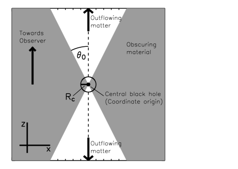
Figure 1: The bi-conical flow geometry under consideration. The outflow (unshaded) has opening angle $\theta_{0}$ and is launched at radius $R_{c}$ from the central black hole. The shaded region is assumed to contain obscuring material through which photons do not propagate. Note that in the limit $\theta_{0}=90$° a spherical outflow with no obscuring material is obtained. The observer is assumed to be at infinity along the positive $z$-axis. The flow is symmetric under rotation about the $z$-axis.

2.1 Velocity and Density

It is assumed that the velocity of the flow increases monotonically outward and is a function of radius ($r$) alone. A simple $\beta$-type velocity law (of the form commonly used in modelling stellar winds) is adopted

$$v(r)=v_{c}+(v_{\infty}-v_{c})\left({1-\frac{R_{c}}{r}}\right)^{\beta}$$ (1)

where $v_{c}$ is the outflow velocity at the base of the wind (i.e. at $r=R_{c}$) and is assumed to be negligibly small; $v_{\infty}$ is the terminal velocity of the flow, which is constrained by the observed line shifts; and $\beta$ controls the rate of acceleration in the wind.

Given the velocity, the mass density $\rho(r)$ is determined by the equation of mass conservation for an outflow with mass-loss rate $\Phi$

$$\rho(r)=\frac{\Phi}{4\pi v(r)r^{2}b}$$ (2)

where $b=1-\cos\theta_{0}$ is the fraction of solid angle subtended by the flow as viewed from the coordinate origin.

2.2 Ionization

The ionization state of all the elements included in the calculation is computed from the radiation field on the assumption of ionization equilibrium. During the Monte Carlo simulations, estimators for the photoionization rate in each bound-free continuum are obtained (following Lucy 2003, see Section 3) and used to compute the ionization state by balancing against radiative recombination rates. Collisional ionization is neglected – this is expected to be a good approximation in view of the intense radiation field and the high ionization potential of the ions important to this study.

The radiative recombination rates depend on the local electron energy distribution. Since thermal balance is not pursued here, this energy distribution is not calculated in detail but is assumed to be Maxwellian with a fixed electron temperature, $T_{e}$. The adopted value of $T_{e}$ is discussed in Section 5.

2.3 Excitation

All the X-ray spectral lines of interest are ground state transitions and so the excitation of levels above the ground state has little effect on the calculations. Therefore the following prescription for excitation is adopted

$$\begin{array}[]{cccc}{n_{i}}/{n_{g}}&=&\left({{n_{i}}/{n_{g}}}\right)^{*}_{T_{r}}&\mbox{if level $i$ is metastable}\\ \\ {n_{i}}/{n_{g}}&=&W(r)\left({{n_{i}}/{n_{g}}}\right)^{*}_{T_{r}}&\mbox{otherwise}\end{array}$$ (3)

where $n_{i}$ is the level population (number density) for an excited state $i$, $n_{g}$ is the population of the ground state and $T_{r}$ is a chosen radiation temperature. The geometric dilution factor is given by $W(r)=\frac{1}{2}(1-\sqrt{1-(R_{c}/r)^{2}})$ and the notation $(\;)^{*}_{T_{r}}$ indicates that the quantity in parenthesis should be evaluated in LTE at temperature $T_{r}$. In practice, $T_{r}$ is set equal to $T_{e}$ throughout.

2.4 Incoming broadband spectrum

Figure 2: The form of the input spectrum of radiation energy. The three distinct components are indicated in the figure.

The Monte Carlo simulations require that the incoming energy spectrum at the base of the wind be specified. In this paper, the incoming spectrum consists of three distinct components (see Figure 2). Energetically, the dominant component is that of the accretion disk around the central black hole. This component is modelled by a simple multi-colour black-body spectrum (Mitsuda et al. 1984). The spectral energy distribution of the disk was obtained from equation 4 of Mitsuda et al. (1984) with the disk inner radius $r_{\mbox{\scriptsize in}}=3R_{s}$ and the outer radius $r_{\mbox{\scriptsize out}}=100R_{s}$ ($R_{s}$ is the Schwarzchild radius of the black hole). Since PG1211+143 is believed to be accreting at, or close to, the Eddington limit (Boroson 2002, Gierliński & Done 2004), the total disk luminosity was fixed at the Eddington luminosity. The mass of the central black hole, which is required for the calculation of $R_{s}$ and the Eddington luminosity, is taken to be $4\times 10^{7}$M_⊙ (Kaspi et al. 2000).

At hard X-ray wavelengths the continuum spectrum is well described by a simple power law which most probably arises through inverse Compton scattering of seed disk photons in an optically thin region in or near the disk. The formation of this power law is not addressed here but it is included as part of the input spectrum. The photon power law index $\Gamma=1.75$ is adopted (the observed index for PG1211+143 has been determined by Pounds et al. [2003a] from both XMM-Newton pn and MOS data yielding respectively $\Gamma\sim 1.79$ and $\Gamma\sim 1.71$). The normalisation of the power-law component relative to that of the disk is chosen in order to obtain consistency with the observed X-ray (2 – 10 keV) luminosity. To achieve this, the normalisation is adjusted iteratively in the Monte Carlo calculations (see Section 3.6).

At soft X-ray energies a significant excess of emission is observed relative to the power-law component (Pounds et al. 2003a). This soft-excess is included in the input spectrum here. Its shape is modelled by a black-body with temperature $T=1.3\times 10^{6}$ K, the temperature of the primary black-body component fitted to the spectrum by Pounds et al. (2003a). The normalisation of this component is fixed to that of the power-law by the observation that the intensity of the soft-excess component is approximately equal to that of the hard power-law at $\sim 0.8$ keV (see figure 3 of Pounds et al. 2003a). An excess of emission in the soft X-ray band is common in quasars but its origin is not well understood (see e.g. Gierliński & Done [2004] for a recent discussion). For the purposes of this paper, however, the soft excess is of relatively little concern since it is not a major contributor to the hard X-ray region.

3 Monte Carlo simulations

The code used to perform radiative transfer calculations is based on that discussed by Sim (2004) which uses the Macro Atom formalism recently developed by Lucy (2002,2003). The principles of the code are briefly discussed below, with particular emphasis on those aspects that differ from the Sim (2004) code.

3.1 Geometry

The code adopts a bi-conical geometry with opening angle $\theta_{0}$ (see Section 2 and Figure 1). In practise the radiative transfer calculation is performed in one cone and then the relevant parameters of the flow (e.g. the mass-loss rate $\Phi$) are doubled to account for the bi-conical structure. Energy packets are launched through the surface at the base of the cone (radius $R_{c}$ from the black hole) and their propagation through the cone is tracked in both radial ($r$) and angular ($\theta$) position until they leave the flow through the outer boundary at $r=r_{\mbox{\scriptsize max}}$ or the conical boundary at $\theta=\theta_{0}$. The lower boundary $r=R_{c}$ is assumed to be reflecting so that no packets are lost through this surface. Packets which pass through the outer boundary $r=r_{\mbox{\scriptsize max}}$ are assumed to escape to infinity while those that pass through the conical boundary are assumed to be destroyed by obscuring material (such as might be present in the form of a dusty torus surrounding the AGN [Antonucci & Miller 1985, Pier & Krolik 1992], or the warm highly ionized medium [WHIM] discussed by Elvis [2000]). It is assumed that no photons enter the flow through the conical boundaries. In practise there would be little effect if photons did enter via these boundaries provided that they are not hard enough to influence the ionization state of the material in the flow.

3.2 Discretization of the model

The flow is divided into 100 cells in the radial direction equally spaced in $x=R_{c}/r$. The outermost cell extends to $r_{\mbox{\scriptsize max}}=100R_{c}$. At present there is no angular ($\theta$) stratification.

3.3 Propagation and interaction of packets

The propagation of packets through the model is followed exactly as described by Sim (2004). The treatment of line interactions using the Sobolev approximation and the Macro Atom formalism is also as described by Sim (2004), with the exception that bound-free processes are now included in the Macro Atom description. Thus, in contrast to the photoionization modelling described by Pounds et al. [2003a], the linewidths and profiles are computed rather than pre-specified.

Following the formalism developed by Lucy (2003), the calculations presented here include bound-free absorption and emission (including the creation and destruction of $k$-packets) which were neglected by Sim (2004). In addition, since X-ray photons are under investigation, electron scattering is no longer treated in the limit of Thompson scattering but is generalised to account for Compton scattering as described in the next subsection.

3.3.1 Compton scattering

The electron scattering cross-section presented to an $r$-packet is computed using the Klein-Nishina equation for the differential cross-section on the assumption that the target electrons are stationary in the co-moving frame (see e.g. Leighton 1959).

When electron scattering occurs, the scattering angle is selected from a pre-tabulated look-up table of the angular probability distribution as a function of incident photon energy using the Klein-Nishina equation.

Physically, when a photon undergoes Compton scattering some fraction of its energy ($f$, which is readily related to the photon frequency and scattering angle) is passed to the electron, reducing the frequency, and therefore energy, of the photon. However, such a splitting of energy is not desirable in the context of the “indivisible energy packet” approach adopted here. Therefore $f$ is identified as the probability that during a Compton scattering event the $r$-packet is converted insitu to a $k$-packet (which is subsequently eliminated by thermal cooling processes in the usual way) and $1-f$ is the probability that the packet will continue to propagate as an $r$-packet with diminished frequency but unchanged energy (in the co-moving frame). When averaged over many interactions, this approach reproduces the physics of Compton scattering exactly without the need to divide energy packets at any point.

It is noted that this scheme for the treatment of Compton scattering assumes that the electron rapidly comes back into thermal equilibrium with its surroundings following the interaction with the photon. This assumption is adequate here but in principle could be lifted to allow the energy carried by non-thermal electrons to be followed during Monte Carlo simulations when necessary. This is likely to be important when the methods are generalised to include inverse Compton scattering.

3.4 Monte Carlo estimators

For the formal calculation of the emergent spectrum (see Section 3.7), Monte Carlo estimators are needed not only for the Sobolev mean intensity in the spectral lines ($\bar{J}$, given by equation 10 of Sim [2004]) but also for the mean intensity in both the far blue ($J^{b}$) and red ($J^{r}$) wings of the lines and also for a weighted mean intensity in the far blue wing ($J^{b,\tau}\equiv<I^{b}e^{-\tau_{s}}>$, where $I^{b}$ is the specific intensity in the far blue wing, $\tau_{s}$ is the Sobolev optical depth and $<...>$ indicates an angular average). Estimators for these quantities in each cell are readily constructed following Lucy (1999, 2003):

$$J^{b}=\frac{1}{4\pi\Delta t}\frac{1}{V}\sum_{\mbox{\scriptsize in}}\frac{1}{\mbox{d}\nu/\mbox{d}s}\epsilon$$ (4)

$$J^{r}=\frac{1}{4\pi\Delta t}\frac{1}{V}\sum_{\mbox{\scriptsize out}}\frac{1}{\mbox{d}\nu/\mbox{d}s}\epsilon$$ (5)

$$J^{b,\tau}=\frac{1}{4\pi\Delta t}\frac{1}{V}\sum_{\mbox{\scriptsize in}}\frac{e^{-\tau_{s}}}{\mbox{d}\nu/ds}\epsilon$$ (6)

In each case $\Delta t$ is the time interval represented by the Monte Carlo simulation, $V$ is the volume of the cell in question, $\epsilon$ is the packet energy and $\mbox{d}\nu/\mbox{d}s$ is the gradient of co-moving frequency with path-length. In the first and third cases the summation runs over all packets as they redshift into resonance with the line and in the second case the summation is over packets as they redshift out of resonance with the line.

In principle, Monte Carlo estimators for the photoionization rate and stimulated recombination rate ($\gamma$ and $\alpha^{\mbox{\scriptsize st}}$) should be obtained using equations 44 and 45 of Lucy (2003). However, since the line estimators presented above provide a closely spaced grid of values for $J$ in each cell it is possible to obtain $\gamma$ and $\alpha^{\mbox{\scriptsize st}}$ by integrating over this grid. This method has been adopted since it noticeably reduces the run time of the code (when the bound-free estimators are computed directly a significant fraction of computer time is spent on recording the large number of small contributions to these estimators which arise because of the large number of electron scattering events). Although estimators obtained by this approach are slightly less accurate than those obtained with equations 44 and 45 of Lucy (2003), they are still of higher quality than those for the individual lines and since it is necessary to simulate a large enough number of packets that the line estimators are reliable, then it is acceptable to compute the bound-free estimators from the line estimators and obtain a similar degree of accuracy.

3.5 The time interval

The time interval represented by the Monte Carlo simulation, $\Delta t$ is determined by the observed 2 – 10 keV luminosity, $L_{\mbox{\scriptsize X}}=3.3\times 10^{43}$ ergs s^-1 for PG1211+143 (Pounds et al. 2003a). During the Monte Carlo simulation, the total energy in the 2 – 10 keV energy band carried by packets through the outer boundary of the model ($E_{\mbox{\scriptsize X}}$) is recorded and used to obtain the time interval via

$$\Delta t=\frac{E_{\mbox{\scriptsize X}}}{bL_{\mbox{\scriptsize X}}}$$ (7)

where, as usual, $b$ is the fraction of solid angle subtended by the flow. The time interval ($\Delta t$) is used both for the normalisation of the Monte Carlo estimators (see Section 3.4) and for determining the relative normalisation of the power-law and disk components of the input spectrum in the next iteration.

3.6 Iteration cycle

Each complete run of the code involves several iterations of the Monte Carlo calculation to converge the Monte Carlo estimators, ionization fractions and the relative normalisation of the disk and power-law components of the input spectrum. Initially it is assumed that the flow is fully ionized and a Monte Carlo simulation (with a relatively small number of energy packets) is performed to obtain preliminary values for the photoionization rates. These are used to compute more realistic ionization fractions before performing additional Monte Carlo simulations. In each successive simulation the Monte Carlo estimators obtained from the previous simulation are used to compute the ionization fractions and the Macro Atom jumping/de-activation probabilities. Also, the time interval (Section 3.5) is used to obtain the relative normalisation of the components of the input radiation field. Typically five iterations were performed to converge the final values of the estimators to sufficient accuracy for the spectral synthesis step described below.

3.7 Spectral synthesis

While it is possible to produce spectra from Monte Carlo simulations directly by examining the frequency distribution of the energy packets emerging from the computational domain, it has been demonstrated by Lucy (1999) that far higher quality spectra may be obtained by using the Monte Carlo estimators to perform a formal integral solution of the transfer equation. The accuracy of the spectrum generated in this manner is limited not by the Monte Carlo noise in the outgoing packet frequency distribution but by the Monte Carlo noise in the estimators which is significantly lower. A brief discussion of the method of spectral synthesis is given below with particular attention given to the differences from Lucy (1999).

3.7.1 Ray tracing

To compute the outgoing spectrum, the specific intensity at each frequency $I_{\nu}$ is traced along a set of paths through the model with a range of impact parameters. The total emergent intensity is determined by numerical integration over the impact parameter (see Lucy 1999). It is assumed that the observer lies directly above the axis of symmetry of the flow (the line $\theta=0$). Initially, the intensity of the ray is either set to that of the input radiation field (if the impact parameter is sufficiently small that the ray trajectory originates on the inner surface boundary at $R_{c}$) or to zero (if the impact parameter is large enough that the ray originates on either the conical boundary [bi-conical models] or the outer edge of the rear hemisphere [spherical models]). The intensity of the beam is then traced along the path to the edge of the model in the following way. First, the distance the ray must travel until the comoving frequency of the photons with which it is associated becomes redshifted into a spectral line is found. The continuum optical depth $\tau_{c}$ and source function $S_{c}$ are computed for this path length, including contributions from both electron scattering and bound-free processes. The continuum source function is given by

$$S_{c}=\frac{\tau_{es}}{\tau_{c}}S_{es}+\frac{\tau_{bf}}{\tau_{c}}S_{bf}$$ (8)

where $\tau_{es}$ and $\tau_{bf}$ are the optical depths due to electron scattering and bound-free processes respectively. Since the ionization fractions have already been computed from the radiation field and the important bound-free processes all involve recombinations from ground states, the bound-free source function $S_{bf}$ is computed directly from the ionization fractions in the usual way. The source function for electron scattering is assumed to be isotropic and given by the mean intensity, $J$, which is obtained by interpolation between the value of $J^{r}$ for the next spectral line to the blue and $J^{b}$ for the next spectral line to the red (in the comoving frame). The values of $J^{r}$ and $J^{b}$ are already determined by the estimators discussed in Section 3.4. Once the intensity is known at the point where the ray is redshifted into a spectral line, the effect of the line on the intensity of the ray is accounted for using

$$I^{r}_{\nu}=I^{b}_{\nu}e^{-\tau_{s}(\mu)}+S_{bb}(1-e^{-\tau_{s}(\mu)})$$ (9)

where $I^{b}_{\nu}$ is the incoming intensity at the far blue wing of the line, $I^{r}_{\nu}$ is the outgoing intensity at the far red wing of the line, $S_{bb}$ is the line source function and $\tau_{s}(\mu)$ is the Sobolev optical depth of the line (which depends on $\mu$, the cosine of the angle between the ray direction and the radial direction). Since level populations are not computed self-consistently then it is not appropriate to compute $S_{bb}$ from the level populations but rather from the Monte Carlo estimators for the radiation field. This is achieved by averaging the above equation over $\mu$ to obtain an expression for $S_{bb}$ in terms of mean intensities

$$S_{bb}=\frac{J^{r}-J^{b,\tau}}{\frac{1}{2}\int_{-1}^{+1}(1-e^{-\tau_{s}(\mu)})\;\mbox{d}\mu}$$ (10)

Since estimators have been recorded for both $J^{r}$ and $J^{b,\tau}\equiv<I^{b}_{\nu}e^{-\tau_{s}}>$ (see section 3.4) this allows $S_{bb}$ to be evaluated without reference to the level populations. Once the ray has passed though resonance with the line, the distance to the next line is computed and the effects of continuum opacity up to that line are accounted for as before. This processes of alternately accounting for the continuum and lines is continued until the ray reaches the top of the model whereupon the outgoing intensity is recorded and used to compute the spectrum. In practise, since the X-ray region is relatively sparsely populated with spectral lines, the gridding obtained for the computation of the electron scattering source function is rather coarse. This is easily overcome by introducing additional fake spectral lines in the Monte Carlo simulation. These are defined to have zero optical depth and so do not affect the propagation of energy packets but they do cause $J$ to be computed on a finer frequency mesh, as required.

3.8 Accuracy of the calculations

The number of energy packets used in each simulation is chosen in order that the Monte Carlo noise in the estimators is $<10$ per cent. This level of precision is sufficient given the limited quality of the observational data available at present. To this accuracy, the transformation between the comoving and observer rest frame can be taken as Galilean and the Doppler shift treated as non-relativistic. If higher accuracy were to be required it would become necessary to consider special relativistic corrections (which are of order $v/c\leq 0.1$). Including such corrections poses no significant problems to the operation of the code but in view of the precision required here they can be neglected for simplicity.

4 Atomic data

Table 1 lists the elements and ions included in the calculations described below. For light elements only hydrogen- and helium-like ions are included, but lower ionization stages are included for iron and nickel. The element abundances, relative to hydrogen, are assumed to be solar. Atomic models, bound-bound oscillator strengths and bound-free cross-sections have been extracted from the Xstar database (Bautista & Kallman 2001). In the calculations, all the bound-bound transitions in the database for the ions listed in Table 1 are included, a total of $\sim 2500$ lines. For hydrogen-like ions, bound-free transitions from levels with $n=1,2,3$ and 4 are included. For helium-like ions, bound-free transitions from the 1s², 1s2s, 1s2p and 1s3s configurations are included. For all other ions, photoionization is included for all those of the ten lowest lying fine-structure energy levels for which cross-sections are given in the database. In total $\sim 250$ bound-free continua are included in the calculations.

Table 1: The elements and ions included in the calculations.

Element	Ions	Element	Ions
H	i, ii	Si	xiii – xv
He	i – iii	S	xv – xvii
C	v – vii	Ar	xvii – xix
N	vi – viii	Ca	xx – xxii
O	vii – ix	Fe	xxiii – xxvii
Ne	ix – xi	Ni	xxvi – xxix
Mg	xi – xiii

Figure 3: 2 – 10 keV energy spectra computed from spherical ($b=1$) models with (top to bottom) $\Phi=1$, 3, 6 and 10 M_⊙ yr^-1 (solid curves). The energy is measured in the quasar rest-frame. In each case $T_{e}=1.3\times 10^{6}$ K. The strongest spectral lines are identified in the figure. The dashed lines show continuum spectra, computed in the absence of bound-free processes and spectral lines.

5 Results

5.1 Spherical flow models

Pounds et al. (2003a) suggest that the outflow from PG1211+143 may have a relatively wide opening angle and so it is instructive to begin with the consideration of the simplest wind geometry, that of spherical outflow (i.e. $\theta_{0}=90$°, hence $b=1$).

5.1.1 Model parameters

In addition to the specification $\theta_{0}=90$°, there are five parameters that must be chosen: $v_{\infty}$, $R_{c}$, $\beta$, $T_{e}$ and $\Phi$ (see Section 2 for definitions of these quantities).

The observed line shifts constrain $v_{\infty}$ directly. In all models discussed here, $v_{\infty}=0.1c$ is adopted which is characteristic of the line shifts measured in both PG1211+143 and PG0844+349 by Pounds et al. (2003a,b).

It is reasonable to speculate that $R_{c}$ should be at least the radius of the last stable orbit around a Schwarzchild black hole (i.e. $R_{c}>3R_{s}$ where $R_{s}$ is the Schwarzchild radius). Moreover, it is a general characteristic of winds in most astrophysical systems that the terminal velocity is comparable to the escape velocity in the region from which the wind is launched. Given the choice $v_{\infty}=0.1c$, this argument suggests $R_{c}=100R_{s}$ is appropriate, a value which is adopted throughout this investigation.

In the absence of information on the probable shape of the velocity law in the flow, $\beta=1/2$ is adopted in all models. This value is theoretically attractive since it arises for the particular case that the driving force has the same radial dependence as gravity and it is close to characteristic values for radiatively driven flows in other astrophysical objects (e.g. $\beta\sim 0.7$ in O stars [Groenewegen & Lamers 1989]). There are objects for which significantly larger values (e.g. $\beta\sim 3$ for Wolf-Rayet stars [see Ignace, Quigley & Cassinelli 2003 and references therein]) have been suggested but values much smaller than $\beta=1/2$ seem improbable for radiatively driven flows.

As standard, $T_{e}=1.3\times 10^{6}$ K is adopted. This value is based on the primary black-body temperature fitted to the observed soft X-ray excess in PG1211+143 (Pounds et al. 2003a). The choice of $T_{e}$ does not qualitatively affect the computed spectrum, but it does quantitatively influence the equivalent widths of spectral features. In principle, if all important heating and cooling processes were included in the calculation, $T_{e}$ could be computed rather than assumed. However, this goes beyond the scope of this paper in which the primary objective is spectral synthesis. To indicate the sensitivity of the results presented here to $T_{e}$, the Appendix briefly discusses models with temperatures both higher and lower than the standard temperature adopted here.

The mass-loss rate, $\Phi$ is one of the primary unknowns in this investigation. Based on simple fits to the XMM-Newton data, Pounds et al. (2003a) suggest a mass-loss rate $\Phi\sim 3$ M_⊙ yr^-1. For this investigation, calculations have been carried out for spherical models with $\Phi=1$, 3, 6, and 10 M_⊙ yr^-1. The results of these calculations are presented in the next section.

Table 2: Equivalent width (EW) and full-width at half-maximum (FWHM) for the computed absorption components of the S xvi and Mg xii Lyman $\alpha$ lines and the combined Fe xxvi/xxv feature at 7.5 keV for spherical wind models ($\theta_{0}=90$°, $b=1$). The last row in the table gives the observational constraints taken from Pounds et al. (2003a). The last column of the table gives the radius in the outflow at which the electron scattering optical depth $\tau_{e}=1$ in the radial direction. The Monte Carlo simulations are accurate to about $\pm 10$ per cent in EW and $\pm 300$ km s^-1 in FWHM.

Model	Fe (7.5 keV)		S xvi Lyman $\alpha$		Mg xii Lyman $\alpha$		$r(\tau_{e}=1)$
$\Phi/b$	EW	FWHM	EW	FWHM
(M⊙ yr-1)	(eV)	(km s${}^{-1})$	(eV)	(km s-1)	(eV)	(km s-1)	($R_{s}$)
1.0	140	21,000a	–b	–b	–b	–b	100
3.0	360	21,000a	10	7,400	–b	–b	200
6.0	380	20,000a	19	5,300	6	4,800	370
10.0	280	16,000a	30	4,500	8	4,000	590
Observations	$95\pm 20$	$\sim 12,000$	$32\pm 12$		$15\pm 6$

^a To obtain a single FWHM for the Fe blend at 7.5 keV, the computed spectrum was convolved with a Gaussian of FWHM = 10,000 km s^-1. The FWHM reported in the table is that measured from the convolved spectrum.

^b In some cases, several of the lines do not appear or are too weak for reliable calculation of their profiles above the Monte Carlo noise.

5.1.2 Computed spectra and discussion

Figure 3 shows spectra computed in the 2 – 10 keV region from models with the standard parameters discussed above and the four values of $\Phi$ under consideration (1, 3, 6 and 10 M_⊙ yr^-1). In each case, the continuum level as computed in a separate run of the code in which only Compton scattering by electrons is considered (i.e. no bound-free continua or lines are included) is plotted for comparison.

These model spectra are rather encouraging: in all four cases they are consistent with the observations in that the strongest absorption feature is, by a considerable margin, due to the Lyman $\alpha$ line of hydrogen-like iron (Fe xxvi) and the 1s – 2p resonance line of helium-like iron (Fe xxv). Comparing the four spectra plotted in Figure 3 shows that as the mass-loss rate is increased the Fe xxv line becomes stronger relative to the Fe xxvi line. This is a consequence of the response of the iron ionization balance to the density – higher densities favour formation of the lower ionization species. The ionization balance is discussed further in Section 5.2.

At the lowest densities considered ($\Phi=1$ M_⊙ yr^-1) the blended iron feature is the only strong feature in the spectrum. At higher densities weak lines appear at lower energies, most importantly the Lyman $\alpha$ lines of hydrogen-like silicon and sulphur. The sulphur line is observed in PG1211+143 but the region around the silicon line is marred by instrumental effects in the data preventing a firm identification (Pounds et al. 2003a). The Lyman $\alpha$ line of hydrogen-like magnesium is also present in the data. The high density models do predict this feature but it is always weak.

Various absorption features appear at energies above $\sim 8.5$ keV and become stronger as the density is increased. Most prominent of the high energy ($>8$ keV) absorption features is the 1s – 3p resonance line of Fe xxv but there are several other contributers to the absorption including the Fe xxvi Lyman $\beta$ line (at around 9 keV), the ground state photoionization edges of Fe xxv and xxvi and lines of Ni xxvii and xxviii. In the observations of PG1211+143 (Pounds et al. 2003a) an absorption line is detected at $\sim 8.7$ keV but it is less statistically significant than the stronger feature at $\sim 7.5$ keV.

In addition to blueshifted absorption there is some weak redshifted emission associated with several of the features. This appears in the spherical models because there is no obstruction to observing the receding back hemisphere of the flow. These emission features are largely absent from the spectra computed from bi-conical models (Section 5.2) in which the receding flow is obscured.

For quantitative comparison, Table 2 gives the equivalent width and full-width at half-maximum (FWHM) of the iron feature at 7.5 keV and the observed S xvi and Mg xii Lyman $\alpha$ lines for the model spectra. None of the spherical models predict strong, sharp absorption lines due to lower ionization elements at softer energies (e.g. the O viii Lyman $\alpha$ line). Since the Fe xxvi and Fe xxv components of the 7.5 keV feature are not separately identified in the data, these two lines are considered as one blended feature. To determine a single FWHM for this feature, the computed spectra were convolved with a Gaussian of FWHM = 10,000 km s^-1 to simulate the XMM-Newton resolution. The tabulated width is that obtained from the convolved spectrum. For completeness, the table also gives the radial position in the flow at which the optical depth due to electron scattering ($\tau_{e}$) is unity in the radial direction (this is the definition used for the “photospheric” radius by Pounds et al. [2003a] and King & Pounds [2003]).

Figure 4: As Figure 3 but showing results for bi-conical models with $\theta_{0}=60$° ($b=0.5$).

Figure 3 and Table 2 show that the sulphur and magnesium lines become stronger and narrower as the mass-loss rate is increased. It is apparent from Figure 3 that as the density is increased the two components of the iron 7.5 keV feature also become narrower. However, the width of the combined feature (see Table 2) does not vary much until the density is high enough that only the Fe xxv component is strong.

Although encouraging for the reasons discussed above, the spherical models have problems when confronted by the data. The high mass-loss rate models ($\Phi=6.0$ and 10 M_⊙ yr^-1) can be easily ruled out based on their predicted spectra at $>8$ keV: these models favour a rapid decline in hard X-ray flux as a function of energy which is not supported by the observations. This predicted decline occurs as a result of both multiple Compton scattering and absorption by spectral lines and continua.

In the lower mass-loss rate models, the 7.5 keV iron feature is slightly too strong while the sulphur and magnesium Lyman $\alpha$ lines are too weak or absent. Also, these models do not predict significant absorption by the Lyman $\alpha$ lines of hydrogen-like carbon, nitrogen or oxygen. These lines have been detected in the RGS spectrum of PG1211+143 (Pounds et al. 2003a) and have similar blueshifts to the hard X-ray lines, suggesting that they may form in the same outflow.

In addition, the linewidths of the features in the low density models are likely to be too large. The 7.5 keV iron feature is unresolved in the data, implying that its width should be $\leq 12,000$ km s^-1 (Pounds et al. 2003a). For all but the highest density model, the predicted width of the feature at 7.5 keV is noticeably greater than this. It is important to note, however, that the widths of the two lines individually (Fe xxvi Lyman $\alpha$ and Fe xxv 1s–2p) are significantly smaller than that of the blended feature. Therefore if the observed line corresponds to only one of the computed K $\alpha$ features (as suggested by Pounds et al. 2003a) the widths are compatible. The sulphur and magnesium lines are predicted to be significantly narrower than the iron line. Constraints on the widths of these lines are not provided by the data. However, profiles of lines arising from lower ionization ions in the soft X-ray RGS spectrum suggest linewidths $\leq 2,000$ km s^-1 (Pounds et al. 2003a). The widths of the soft X-ray lines do not place direct constraints on the properties required of hard X-ray spectral features but if the sulphur and magnesium Lyman $\alpha$ lines form under similar conditions to lines observed at softer energies (e.g. the observed O viii Lyman $\alpha$ line) it is to be expected that their linewidths should be comparable. This is weak additional evidence against the low density spherical models.

Given the quality of the data and the various model uncertainties (including the element abundances) it is unreasonable to expect very good quantitative agreement but it is worthwhile to search for model conditions which might reproduce the observed properties of the spectrum more accurately. In the next section it is shown that improvements can be obtained by lifting the assumption of sphericity and considering bi-conical flows such as discussed by Pounds et al. (2003a) and King & Pounds (2003).

5.2 Bi-conical flow models

Figure 5: As Figure 3 but showing results for bi-conical models with $\theta_{0}=30$° ($b=0.13$).

Models in which $\theta_{0}<90$° ($b<1$) are now considered and contrasted with the spherical models discussed above.

5.2.1 Model parameters

Throughout this section the parameters $v_{\infty}$, $R_{c}$, $\beta$ and $T_{e}$ remain fixed at the values used for the spherical models. Spectra are computed for models with $\theta_{0}=60$°  ($b=0.5$) and $\theta_{0}=30$°  ($b=0.13$). For both values of $\theta_{0}$, models with four values of $\Phi$ have been considered. For ease of comparison between the models, the values of $\Phi$ adopted are chosen to give the same densities as in the spherical models rather than the same total mass-loss rates (i.e. the values of $\Phi$ considered are such that $\Phi/b=1$, 3, 6 and 10 M_⊙ yr^-1).

5.2.2 Computed spectra and discussion

Figures 4 and 5 show the spectra computed from models with $\theta_{0}=60$° and 30°  respectively. Individually, Figures 4 and 5 show similar trends in the spectra as a function of density as the spherical models in Section 5.1.

More interestingly, by comparing Figures 3, 4 and 5, it is apparent that as $\theta_{0}$ is reduced, the iron feature at 7.5 keV remains strong but both components of the absorption become sharper and the relative strength of the Fe xxv and xxvi features varies with $\theta_{0}$ such that the higher ionization line is strongest when the opening angle is smallest.

Figure 6: Detail of the computed O viii, Mg  xii and S xvi Lyman $\alpha$ line profiles for the highest density models ($\Phi/b=10$ M_⊙ yr^-1). The spectra are normalised to the continuum. In each panel, the solid curve shows results for $\theta_{0}=90$° (spherical flow), the dashed curve for $\theta_{0}=60$° ($b=0.5$), and the dotted curve for $\theta_{0}=30$° ($b=0.13$). The labels identify the line positions at the terminal velocity of the outflow. The solid vertical lines indicate the rest energies of the lines. The small scale structure that can be seen at the level of $\sim 5$ per cent is Monte Carlo noise in the simulations.

The opening angle has a more significant effect on the weaker, lower energy lines. To illustrate this influence Figure 6 compares the S xvi, Mg xii and O viii Lyman $\alpha$ line profiles from the highest density models ($\Phi/b=10$  M_⊙ yr^-1) for different values of $\theta_{0}$ in detail. The calculations reveal an interesting trend: as $\theta_{0}$ is reduced these lines become narrower and deeper, bringing them into significantly closer agreement with the constraints placed on the line profiles by the observations. The rapidity of this effect is inversely correlated with the ionization potential of the species: the relatively low ionization O viii Lyman $\alpha$ line at 0.72 keV, which is the strongest of the lines of various hydrogen-like elements identified by Pounds et. al (2003a) in their RGS data, shows more dramatic variations than the intermediate ionization Mg xii and S xvi lines.

The dependence of the spectral features on both $\theta_{0}$ and $\Phi/b$ can be readily understood in terms of the influence of these model parameters on the computed ionization structure of the wind. To illustrate this, Figure 7 shows the ionization fractions of S xvi and S xv in four models (combinations of $\theta_{0}=90$° [spherical] or 30° with $\Phi/b=1.0$ or 6.0 M_⊙ yr^-1).

Figure 7: Ionization fractions of S xvi (solid curves) and xv (dotted curves) as a function of $x=R_{c}/r$ where $r$ is the radial distance from the central black hole. The four panels correspond to models with $\Phi/b=1$ M_⊙ yr^-1 and $\theta_{0}=90$°  (upper left), $\Phi/b=6$ M_⊙ yr^-1 and $\theta_{0}=90$°  (upper right), $\Phi/b=1$ M_⊙ yr^-1 and $\theta_{0}=30$°  (lower left) and $\Phi/b=6$ M_⊙ yr^-1 and $\theta_{0}=30$°  (lower right). Ionization fractions of oxygen, magnesium and iron behave in a similar manner to those of sulphur.

Table 3: Equivalent width (EW) and full-width at half-maximum (FWHM) for the computed S xvi, Mg xii and O viii Lyman $\alpha$ lines and the combined Fe xxvi/xxv feature at 7.5 keV for bi-conical wind models. For most strong lines, the Monte Carlo simulations are accurate to about $\pm 10$ per cent in EW and $\pm 300$ km s^-1 in FWHM. The uncertainties are larger for weaker lines. The last row in the table gives the observational constraints taken from Pounds et al. (2003a).

Model		Fe (7.5 keV)		S xvi Lyman $\alpha$		Mg xii Lyman $\alpha$		O viii Lyman $\alpha$
$\Phi/b$	$\theta_{0}$	EW	FWHM	EW	FWHM	EW	FWHM	EW	FWHM
(M⊙ yr-1)	(°)	(eV)	(km s${}^{-1})$	(eV)	(km s-1)	(eV)	(km s-1)	(eV)	(km s-1)
1.0	60	160	25,000a	–b	–b	–b	–b	–b	–b
1.0	30	130	22,000a	–b	–b	–b	–b	–b	–b
3.0	60	310	17,000a	8	4,800	$\leq 3$	–b	–b	–b
3.0	30	320	19,000a	8	4,000	3	4,300	0.5	2,300
6.0	60	370	18,000a	18	3,800	7	3,300	$\leq 2$	–b
6.0	30	350	18,000a	17	2,800	7	2,800	2	1,500
10.0	60	320	17,000a	24	3,300	8	3,300	3	1,500
10.0	30	340	18,000a	23	2,500	9	2,000	4	1,800
Observations		$95\pm 20$	$\sim 12,000$	$32\pm 12$		$15\pm 6$		$4.2\pm 0.9$	$<2,000$

^a To obtain a single FWHM for the Fe blend at 7.5 keV, the computed spectrum was convolved with a Gaussian of FWHM = 10,000 km s^-1. The FWHM reported in the table is that measured from the convolved spectrum.

^b In some cases, several of the lines do not appear as sharp spectral features at the terminal velocity of the flow but are either very weak, broad features or absent. In such cases no values are given in the table.

The absolute value of the ionization fractions at the outer boundary of the wind is primarily determined by the density, a consequence of the requirement placed on the models that the outcoming X-ray flux is consistent with the observed flux. Higher densities favour lower ionization stages, as one would expect.

The model with $\Phi/b=1.0$ M_⊙ yr^-1 and $\theta_{0}=90$° shows very little variation of ionization with $r$ (top left panel of Figure 7). When the density is increased (top right panel of Figure 7) the radiation energy density, and therefore photoionization rate, vary more significantly within the model. This occurs because the higher density leads to a larger opacity (most importantly due to electron scattering) meaning that photons take longer to escape the inner regions. The resulting gradient of photoionization rate with $r$ leads to a gradient of ionization with the highest ionization state in the inner wind.

Similarly, when the opening angle is reduced (lower left panel of Figure 7) a gradient of ionization is introduced. This occurs because of photon leakage through the conical boundary of the flow: many photons which contribute to the energy density in the inner flow leave the domain of the calculation via the conical boundary before reaching the outer parts and therefore never contribute to the energy density at large radii. This physical effect is solely due to the geometry and is an important discriminant between spherical and conical outflow in this, and potentially other, astrophysical applications.

When a narrow opening angle and high density are combined a very dramatic gradient of ionization is produced (lower right panel of Figure 7).

These gradients of ionization are responsible for the narrower line profiles at high densities and small opening angles: a steep gradient concentrates the line opacity in the outer part of the wind making the lines sharper. Differences in the relative strengths of the Fe xxvi and xxv features at a given $\Phi/b$ are also the result of the sensitivity of the ionization gradient to $\theta_{0}$ since steep gradients favour Fe xxv over Fe xxvi in a smaller volume than shallow gradients.

Photon leakage from the flow is also responsible for changes in the continuum shape at high energies. Comparing the dotted lines (electron scattering only) in Figures 3, 4 and 5, it can be seen that as the opening angle is reduced the continuum curves less significantly at high energies (this is particularly apparent for the highest density cases). The curvature of the continuum arises since Compton scattering preferentially removes high energy photons and replaces them with low energy photons. In spherical models, all the energy packets eventually emerge to contribute to the observed spectrum therefore the maximum enhancement of the low energy intensity is seen for this geometry. In conical models, however, whenever a photon is scattered there is a chance that it will be directed out of the flow. This leads to less enhancement of the low energy intensity and less curvature in the continuum as seen by the observer.

The equivalent widths and FWHM of the important iron, sulphur, magnesium and oxygen lines computed from the bi-conical models are given in Table 3. In the next section, these values will be compared with the observational constraints reported by Pounds et al. (2003a).

5.2.3 Confrontation with observations

Compared with the spherical calculations presented in Section 5.1, the spectra obtained from the bi-conical models are in better agreement with the observations (Pounds et al. 2003a) primarily because, as discussed above, reducing $\theta_{0}$ tends to produce deeper and narrower spectral lines.

As with the spherical models, it remains the case that the hard X-ray iron feature (7.5 keV) is rather too strong in the model spectra (by about a factor of four in equivalent width for most cases). It is possible that this discrepancy is, in part, due to the influence of the strong broad Fe K emission line which is not modelled here but is believed to form by reflection from the inner accretion disk (Pounds et al. 2003a discuss suitable fits for this feature). The Fe K emission line is immediately to the red of the observed absorption line which leads Pounds et al. (2003a) to remark on the possibility that the absorption feature is only the Fe xxvi line and that the Fe xxv component overlaps the Fe K emission feature. If this were the case then it would be expected that the observed equivalent width would be smaller than that computed here. This may be particularly plausible at relatively high densities and narrow opening angles since in such cases the two K $\alpha$ absorption lines are individually rather narrow and quite well separated in the model spectra. It is also noted that any significant departure from solar abundances would directly influence the equivalent width.

The absorption at high energies ($\sim$9 keV) is less in the narrow opening angle models than the spherical models. This is due to a combination of narrower line profiles and less continuum softening by Compton scattering (see Section 5.2.2). The high density models ($\Phi/b=6$ and 10 M_⊙ yr^-1) with $\theta_{0}=60$° still predict too much absorption in this region for consistency with the observations, but at $\theta_{0}=30$° the agreement is closer.

Given the data quality and the relatively subtle differences between several of the model spectra it is not currently possible to make a firm statement of a preferred model. However, taking all the available observational constraints on PG1211+143 together, the spectra computed here suggest a moderately high density in the flow (perhaps $\Phi/b\sim 6$ M_⊙ yr^-1) and a fairly narrow opening angle ($\theta_{0}\leq 30$°). High densities are needed in order to produce the important soft X-ray features (to within a factor of a few of their observed strengths) and a small opening angle ensures narrow lines and limits the absorption at hard ($\sim 9$ keV) energy. Based on their detection of moderately strong O vii emission in the RGS data, Pounds et al. (2003a) favoured a relatively wide opening angle flow ($\sim 80$°). While the computations presented here do not rule out such a scenario they do suggest that it will encounter difficulty in reproducing the observed narrowness of the X-ray features. Unfortunately, the models presented here do not predict any O vii emission since the ionizing radiation field is too strong to permit a significant population of this ion to exist in the flow. If the observed O vii emission truly originates in the same material as the higher ionization state absorption lines, this would suggest an inaccuracy of the ionization balance computed here. Alternatively, it is conceivable that the emission arises, at least in part, from lower ionization material that is physically distinct from the high ionization outflow. A more complete discussion of O vii emission (and absorption) requires detailed investigation of the ionization/recombination balance in oxygen which is deferred to later work.

6 Conclusions

It has been shown that realistic radiative transfer calculations support the proposal that the recently identified X-ray absorption features in PG1211+143 (in particular the strong absorption line observed at $\sim 7$ keV) can be explained in terms of a simply parameterised bi-conical outflow model.

Spectra have been computed for outflows with a range of both mass-loss rate and opening angle. The opening angle determines the extent of photon leakage from the flow which plays an important role in establishing a gradient of ionization in the wind. This affects the strengths of the spectral features providing a useful discriminant between spherical and conical outflow. The calculations presented here favour models in which the flow has a moderately small opening angle $\leq 30$° ($b\leq 0.13$) and mass-loss rate a little larger than that suggested by Pounds et al. (2003a) ($\Phi/b\sim$ 6 M_⊙ yr^-1 is proposed here).

A narrow opening angle suggests interpretation in terms of a collimated disk wind or jet originating from the accretion disk. Such outflows are certainly favoured as elementary components of the structure of quasars and a relatively narrow opening angle bi-conical outflow is consistent with existing models for quasars (e.g. Antonucci & Miller 1985; Elvis 2000, 2004). In particular, in the context of the Elvis (2000) model, one may speculate that the highly ionized outflow modelled here lies in some portion of the polar region bounded by the WHIM. Alternatively the X-ray features may form in the most extremely ionized parts of the WHIM itself.

Given that high velocity outflows may be important for understanding the processes which operate in the cores of quasars, there is a real need for higher quality observational data (such as may be provided by the next generation of X-ray observatories as discussed by Chartas et al. 2003). In particular, it is to be hoped that an increase in spectral resolution such as will be provided by the forthcoming Astro-E2 mission, will allow the study of line profiles in much greater detail than is currently feasible.

As better observational data becomes available, future theoretical work will include a detailed investigation of the various absorption and emission features observed at softer energies. Although the O viii Lyman $\alpha$ line has been discussed here, several of the lower ionization features that are observed (e.g. those of O vii) are not predicted by the models at present. An important step in modelling these features is likely to be self-consistent calculation of the temperature in the models since variation of the temperature through the flow may lead to quantitative changes in the ionization balance owing to its effect on recombination rates. Temperature calculations will also provide insight into the formation of a photosphere in the outflow, which might explain the BBB (Pounds et al. 2003a, King & Pounds), and help constrain the launching radius of the wind ($R_{c}$). Such calculations go beyond the scope of the simple modelling presented here but the influence of the choice of temperature on the hard X-ray spectrum is briefly discussed in the Appendix. It may also become necessary to consider angular ($\theta$) variation of the ionization fractions in the flow, departures from ionization equilibrium, rotation and the influence of viewing angle if the basic bi-conical geometry stands up to tighter observational constraints.

This paper has not addressed the important issue of how high velocity flows may be accelerated. It has been suggested that radiation pressure may be primarily responsible (King & Pounds 2003, Pounds et al. 2003a). Since the source here has been assumed to radiate at the Eddington luminosity it is, by definition, the case that radiation pressure is sufficient to overcome gravity but details of how the flow is accelerated over and above gravity to the terminal velocity warrant investigation. Everett & Ballantyne (2004) have concluded that continuum driving alone cannot account for outflows such as have been proposed by Pounds et al. (2003a). However, the part played by spectral lines in driving an outflow has yet to be quantified. If the flow is radiatively driven by lines and bound-free continua then understanding the driving is closely coupled to modelling the softer parts of the spectrum than have been considered here: the X-ray region is relatively sparse of spectral lines and very preliminary indications from the models presented here suggest that the lines in this region are unlikely to provide a significant fraction of the required outward force.

In conclusion, the spectral synthesis presented in this paper suggests that simple flow models can reproduce the absorption features observed in the hard X-ray spectrum of PG1211+143. However, significant further study, both observational and theoretical, is needed in order that these high velocity outflows and their relationship to the black hole accretion process which lies at the heart of the quasar phenomenon can be understood.

References

Antonucci R. R. J., Miller J. S., 1985, ApJ, 297, 621
Bautista M. A., Kallman T. R., 2001, ApJS, 134, 139
Boroson T. A., 2002, ApJ, 565, 78
Chartas G., Brandt W. N., Gallagher S. C., Garmire G. P.,
ApJ, 2002, 579, 169
Chartas G., Brandt W. N., Gallagher S. C., 2003, ApJ, 595,
85
Elvis M., 2000, ApJ, 545, 63
Elvis M., 2004, in “AGN Physics with the Sloan Digital
Sky Survey”, ASP Conference Series 311, eds.
Richards G. T., Hall P. B., San Francisco: ASP, p.109
Everett J. E., Ballantyne D. R., 2004, to appear in ApJL,
astro-ph/0409409
Gierliński M., Done C., 2004, MNRAS, 349, L7
Groenewegen M. A. T., Lamers H. J. G. L. M., 1989,
A&AS, 79, 359
Ignace R., Quigley M. F., Cassinelli J. P., 2003, ApJ, 596,
538
Kaspi S., Smith P. S., Netzer H., Maoz D., Jannuzi B. T.,
Giveon U., 2000, ApJ, 533, 631
Kaspi S., 2004, to appear in “The Interplay among Black
Holes, Stars and ISM in Galactic Nuclei”, IAU
Symposium 222, eds. Bergmann Th. S., Ho L. C. &
Schmitt H. R., astro-ph/0405563
King A. R., Pounds K. A., 2003, MNRAS, 345, 657
Leighton R. B., 1959, “Principles of Modern Physics”, (New
York: McGraw-Hill), p. 433
Lucy L. B., 1999, A&A, 345, 211
Lucy L. B., 2002, A&A, 384, 725
Lucy L. B., 2003, A&A, 403, 261
Marziani P., Sulentic J. W., Dultzin-Hacyan D., Calvani
M., Moles M., 1996, ApJS, 104, 37
McKernan B., Yaqoob T., Reynolds C. S., 2004, to appear
in ApJ, astro-ph/0408506
Mitsuda K. et al., 1984, PASJ, 36, 741
Pier E. A., Krolik J. H., 1992, ApJ, 399, L23
Pounds K. A., Reeves J. N., King A. R., Page K. L.,
O’Brien P. T., Turner M. J. L., 2003a, MNRAS, 345,
705
Pounds K. A., King A. R., Page K. L., O’Brien P. T.,
MNRAS, 2003b, 346, 1025
Reeves J. N., O’Brien P. T., Ward M. J., 2003, ApJ, 593,
L65
Sim S. A., 2004, MNRAS, 349, 899

Appendix: The influence of electron temperature

Throughout the calculations presented in this paper an electron temperature $T_{e}=1.3\times 10^{6}$ K has been adopted. This temperature was chosen based on the primary black-body temperature obtained from fits to the X-ray spectrum of PG1211+143 by Pounds et al. (2003a) and is close to the temperature used in that paper for the analysis of the observed O vii emission feature.

In principle, the electron temperature in the outflow can be determined by detailed consideration of heating and cooling mechanisms but such computations go beyond the scope this paper which is primarily concerned only with radiative transfer and spectral synthesis.

It is instructive, however, to consider how different choices of temperature may influence the computed spectrum. To this end, Figure 8 shows spectra computed for spherical models with $\Phi=3.0$ M_⊙ yr^-1 and temperatures both above ($T_{e}=2.6\times 10^{6}$ K) and below ($T_{e}=6.5\times 10^{5}$ K) the standard temperature. Computations at the standard temperature are also shown, for comparison. Values of the equivalent widths and FWHM of the 7.5 keV iron feature and the Lyman $\alpha$ line of hydrogen-like sulphur in these spectra are given in Table 4.

Figure 8: 2 – 10 keV spectra computed from spherical models with $\Phi=3$ M_⊙ yr^-1 for different electron temperatures ($T_{e}$). The panels show spectra computed with $T_{e}=2.6\times 10^{6}$ K (upper panel), $T_{e}=1.3\times 10^{6}$ K (middle panel) and $T_{e}=6.5\times 10^{5}$ K (lower panel). The dashed lines show continuum spectra, computed in the absence of bound-free processes and spectral lines.

Table 4: Equivalent width (EW) and full-width at half-maximum (FWHM) for the computed absorption components of the S xvi Lyman $\alpha$ line and the combined Fe xxvi/xxv feature at 7.5 keV for spherical wind models ($\theta_{0}=90$°, $b=1$) with $\Phi=3$ M_⊙ yr^-1 and different temperatures. The Monte Carlo simulations are accurate to about $\pm 10$ per cent in EW and $\pm 300$ km s^-1 in FWHM.

Model	Fe (7.5 keV)		S xvi Lyman $\alpha$
$T_{e}$	EW	FWHM	EW	FWHM
(K)	(eV)	(km s${}^{-1})$	(eV)	(km s-1)
$2.6\times 10^{6}$	250	18,000a	–b	–b
$1.3\times 10^{6}$	360	21,000a	10	7,400
$6.5\times 10^{5}$	370	21,000a	21	7,500

^a To obtain a single FWHM for the Fe blend at 7.5 keV, the computed spectrum was convolved with a Gaussian of FWHM = 10,000 km s^-1. The FWHM reported in the table is that measured from the convolved spectrum.

^b In this case, the sulphur line is too weak for reliable calculation above the Monte Carlo noise.

At higher temperatures the spectral features become weaker while at lower temperatures they become stronger. This is due to the influence of the temperature on the recombination rates – at high temperatures the flow is more highly ionized than at low temperatures. It suggests a degeneracy between high densities and low temperatures but this is lifted when the linewidths are considered – high densities tend to lead to narrower lines (see Table 2) because of the ionization gradient they introduce (see Section 5.2.2) but a low temperature does not change the gradient of ionization and therefore does not cause the lines to become narrower. This means that a simple change in the temperature cannot simultaneously address the shortcomings of the low density spherical models discussed in Section 5.1 (i.e. changing the adopted value of $T_{e}$ will not cause the lines to be both narrower and stronger). However, the temperature does have a quantitative effect on the lines via its influence on the ionization balance.

In the future, calculations will be presented in which the temperature is computed by balancing radiative heating and cooling processes, following e.g. Lucy (2003). Such work will allow for the interesting possibility of variations of $T_{e}$ with $r$: if present, this would affect the gradient of ionization which is central to obtaining narrow line profiles in the models discussed here. It is possible that a steep gradient of electron temperature would permit lower ionization stages to form in the outermost parts of the flow, thereby helping to explain many of the lines observed in the RGS spectrum of PG1211+143.