Sloan Digital Sky Survey Imaging of Low Galactic Latitude Fields: Technical Summary and Data Release

Abstract

The Sloan Digital Sky Survey (SDSS) mosaic camera and telescope have obtained five-band optical-wavelength imaging near the Galactic plane outside of the nominal survey boundaries. These additional data were obtained during commissioning and subsequent testing of the SDSS observing system, and they provide unique wide-area imaging data in regions of high obscuration and star formation, including numerous young stellar objects, Herbig-Haro objects and young star clusters. Because these data are outside the Survey regions in the Galactic caps, they are not part of the standard SDSS data releases. This paper presents imaging data for 832 square degrees of sky (including repeats), in the star-forming regions of Orion, Taurus, and Cygnus. About 470 square degrees are now released to the public, with the remainder to follow at the time of SDSS Data Release 4. The public data in Orion include the star-forming region NGC 2068/NGC 2071/HH24 and a large part of Barnard’s loop.

Subject headings: atlases — catalogs — surveys

1 INTRODUCTION

The Sloan Digital Sky Survey (SDSS) is a 5-band photometric survey of 8500 square degrees of the Northern sky and a concurrent redshift survey of nearly a million galaxies and 100,000 quasars selected from the imaging survey York et al. (2000). The primary purpose of the project is to investigate the large scale structure of the Universe and pursue other extragalactic science. The official survey region therefore largely lies above Galactic latitude $|b|>30^{\circ}$ and was carefully chosen to minimize the effect of the troublesome dust near the Galactic plane. This naturally excludes some of the most beautiful parts of the sky, and those areas of most interest for Galactic science.

However, a significant amount of imaging data has been obtained at low Galactic latitude by SDSS, both during telescope commissioning and for calibration at sidereal times when the main survey region was unavailable. During commissioning, the SDSS camera Gunn et al. (1998) was operational before the telescope control system was stable. The camera data acquisition is carried out in drift-scan or “Time Delay & Integrate” (TDI) mode, with the camera crossing the sky at the sidereal rate; the large field of view ($3^{\circ}$) mandates that this be done along great circles. Accordingly, much of the commissioning work was done by parking the telescope at the Celestial Equator and drift-scanning the sky. During commissioning observations in Fall 1998 (when the South Galactic Polar Cap is available for observation), the drift scanning continued outside the SDSS survey area and passed through NGC 2068 and NGC 2071 in Orion. Many of the commissioning runs produced data of high scientific quality, some of which are part of the SDSS Early Data Release (Stoughton et al., 2002, hereafter EDR), where a detailed description of the imaging data can be found. SDSS Runs 259 and 273 generated targets for spectroscopic commissioning, resulting in the first extremely metal-poor galaxy found by SDSS Kniazev et al. (2003), but have never been made public. Since 1999, additional imaging data at low Galactic latitudes have been obtained for a variety of testing and calibration purposes. However, none of these low-latitude data, external to the SDSS survey area, are included in the SDSS data releases (to date the EDR; the First Data Release, DR1, Abazajian et al.  2003; and DR2, Abazajian et al.  2004). We have reduced and calibrated these data as part of a re-reduction and re-calibration of all the imaging data (“ubercalibration”, Schlegel et al. 2004), and we describe these data in the present paper.

The areas of sky observed are described in Section 2. The data products described herein are very similar to those produced by the SDSS, but differ in photometric calibration and data format. These differences are described in Section 3, and some examples of science applications are briefly discussed in Section 4. The data from 1998-1999 are publicly released with this paper and may be accessed via the WWW. Future data releases will also be accessible at this site.

2 THE DATA

2.1 Sky Coverage

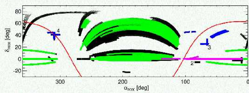
Figure 1: The SDSS footprint in equatorial coordinates, consisting of the (currently released) Orion data (magenta), other Galactic plane runs (blue), SDSS DR2 (green), and other SDSS data taken through December, 2003 (black). Numbers mark the regions shown in Figures 2-4.

The sky coverage of the imaging runs made to date outside the SDSS area is given in Table 1 and Figure 1. The figure shows the footprint of the survey (including these runs) in equatorial coordinates and indicates the approximate locations of images in Figures 2,3, and 4. Table 1 provides information about the location and image quality of each run. An imaging run consists of six long images in each filter, each the width of one CCD ($13.52^{\prime}$ on the sky) and separated by slightly less than one CCD width ($11.65^{\prime}$), produced by the six columns of CCDs in the mosaic camera. A run may last the entire night and be over $100^{\circ}$ long, or can be shorter. A strip is the area covered by the six camera columns from one survey pole to the other; a stripe is a pair of interleaving strips and completely covers a $2.5\times 180^{\circ}$ stripe on the sky. The imaging data are divided into $8.98^{\prime}\times 13.52^{\prime}$ frames for further processing; the aligned frames in the five bands are called a field. Since the sky passes through the u,g,r,i,z SDSS filters in succession (in order r,i,u,z,g) there is a ramp-up time corresponding to 10 frames at the start of each imaging run. Focus and tracking adjustments are made at the beginning of each run, adding variable amounts of overhead to the ramp-up time. The range of fields for each run given in Table 1 define the range of useful data. A detailed description of the observing procedures is given by Gunn et al. (1998) and York et al.  (2000).

The imaging runs comprising the “Orion” data set, released in the present paper, were made in fall 1998 and fall 1999. As Table 1 and Figure 1 show, there have been quite a few low-latitude observations since then, usually for system checking and calibration. Non-photometric data are included, because proper motion studies can make use of the astrometry even in unphotometric runs. The data listed in Table 1 are those which, after reduction and processing, prove to be of science quality, and the photometric reliability is indicated.

2.2 Processing

The SDSS photometric pipeline consists of four sequential steps: ssc and psp (point-spread function estimation), astrom (Pier et al., 2003, astrometry), and frames (object identification, deblending, and photometry; Lupton et al., 2001; Stoughton et al., 2002; Lupton et al., 2003, and in preparation). These pipelines run with little human intervention. The photometric pipeline corrects the imaging data by interpolating over defects such as bad columns and cosmic rays; provides flat-field, photometric and astrometric calibration; and identifies, deblends, measures and classifies objects. The resulting outputs consist of corrected frames, atlas image cutouts for every object, and a catalog of object positions, magnitudes and image classifications in the five SDSS bands. The catalog outputs also include flags which describe the image processing, including whether the object contains any saturated pixels, whether bad data were interpolated over, and whether the object was deblended. Careful attention to these processing flags is critical for proper scientific use of the data. A complete description of the data outputs can be obtained at the above website¹, at the SDSS DR2 web site, and in papers Stoughton et al. (2002); Abazajian et al. (2003, 2004).

The frames pipeline produces a catalog of objects (fpObjc files) described by instrumental quantities: $(x,y)$ positions on a frame, CCD counts, and radii. Astrometric calibrations are applied by the astrometric pipeline (astrom) and are accurate to better than $0.1^{\prime\prime}$ RMS in each coordinate Pier et al. (2003). Because early commissioning data sometimes had poor telescope pointing information (pointing errors of up to $0.5^{\circ}$), astrometric pre-processing using the discrete cross-correlation method described by Hogg et al. (2001) has been performed to allow such data to be processed in an automated fashion. The flat-fielding and photometric calibration were derived from a global recalibration using all of the available repeat imaging (Schlegel et al. 2004). The zero-points of the photometric solutions are forced to agree on average with the calibrations derived from the Photometric Telescope Fukugita et al. (1996); York et al. (2000); Smith et al. (2002) used in SDSS DR2.

2.2.1 Automation with photoop

The importance of a completely automated data processing pipeline cannot be overemphasized; it ensures that all the reductions are carried out in a homogeneous fashion and protects against human biases. Furthermore, it ensures that all reductions are perfectly reproducible, allowing comparisons between different reduction attempts. This is a necessary prerequisite for a survey like the SDSS that targets subsamples of galaxies for follow up observations because it enables one to measure the completeness of these subsamples even as the underlying software evolves.

While the standard SDSS pipelines perform well within the standard survey region, the radically different characteristics of the data near the Galactic plane require adjustments of various pipeline parameters to process these data. In order to implement these in an automated manner, we have developed a meta-pipeline, photoop, to manage all aspects of processing. In production mode, the only human intervention required is to specify the runs to be processed; after that, photoop sets up the photometric pipeline and generates the required input data for each run, including flat-fields, astrometric catalogs, and configuration files. Perl scripts then manage the actual processing across several UNIX servers with a shared NFS file system. Other photoop scripts automate daily maintenance tasks: monitoring the processing status of each run, posting results to an internal web page, and testing data integrity. Notices of pipeline failures and data integrity warnings are automatically sent by email to responsible parties. Furthermore, photoop has been designed to be portable so that anyone with sufficient computing power and access to the raw data can replicate the entire processing system.

2.2.2 Processing Software Versions and Reruns

As the SDSS software pipelines have evolved over time, it has been necessary to keep track of the various processing attempts with rerun numbers. Data processing done via photoop is strictly versioned, with rerun numbers $>100$ to avoid confusion with the main Survey rerun numbers ($0-99$). There is a one-to-one correspondence between rerun number and software versions. The current rerun as of this writing is 137, corresponding to ssc v5_3_4, astrom v3_7, photo v5_4_25, and v4 flatfields and photoop v1_0. For historical reasons, the psp and frames steps of the pipeline are both part of the photo software product. The instructions below for accessing and using the data refer to rerun 137. Future refinements of the software will have higher rerun numbers and will be announced on the website¹.

2.2.3 Calibration

Survey data releases are indirectly calibrated to a set of primary photometric standard stars measured the US Naval Observatory (USNO) 1m telescope in the SDSS filters. This photometric system is denoted by u’,g’,r’,i’,z’ and is defined by Smith et al.  (2002). These primary standards are bright enough to saturate the 2.5m survey telescope, so the photometric system is transfered to a set of secondary standard star “patches” observed by a 20-inch “Photometric Telescope” (PT) situated adjacent to the survey telescope. These secondary standards are used to calibrate the 2.5m native filter system (denoted u,g,r,i,z) to the USNO system for typical star colors. Note that the u’,g’,r’,i’,z’ and u,g,r,i,z systems are significantly different (see e.g. Stoughton et al. 2002). PT patches are sparse or nonexistent for much of the Orion region, so we have instead used the ubercalibration algorithm (Schlegel et al.  2004) to tie the eight Orion runs together photometrically. This algorithm lets the calibration zero-points in each CCD ($a$-terms) and atmospheric extinction ($k$-terms) float night by night, constrained by multiple observations of stars in run overlaps. Run 308 does not overlap any of the other Orion runs, and is therefore calibrated using the same $a$- and $k$-terms as run 307 from the same night. Ubercalibration minimizes the RMS magnitude residuals in repeat observations of $\sim 10^{6}$ stars by adjusting these $a$- and $k$-terms. Because the north and south strips of the equatorial stripe overlap only at the camera column edges, and the flatfields are less certain there, it is necessary to use a perpendicular scan (run 2766) to tie the 12 independent camera columns together. This run is connected to the Orion runs via four other equatorial runs (94, 125, 1755, 2677). For equatorial drift scans the airmass is constant, making the $a$- and $k$-terms degenerate, so $k$-terms are fixed to canonical values.

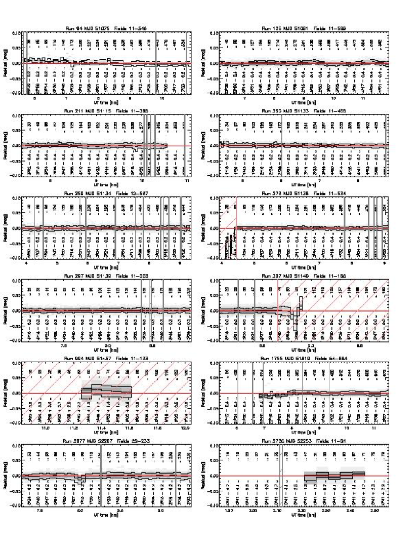
Figure 5: Measured magnitudes minus means for each star of each run used in the Orion ubercalibration (see §2.2.3). Stars brighter than (19.0,19.0,19.0,18.5,17.0) in (u,g,r,i,z) are used in the calibration; results are shown for $r$ band only. Differences are represented as gray scales with 25th, 50th, and 75th percentile lines. Results are similar for g and i bands, with more photometric scatter in u and z bands (see Fig. 6). Cloudy or otherwise unphotometric data are indicated by red cross-hatches, and gray hatches indicate fields where the pipeline was unable to determine a good point spread function; these data are not used in fits. Run 308 does not appear here because it has no overlap with the others, but is calibrated by fixing its parameters to run 307.

Most stars are observed multiple times by this set of runs, and for each star the residual between each run and the mean of all observations of that star is shown in Figure 5. Only stars with $7.43^{\prime\prime}$ radius aperture magnitudes brighter than (19.0,19.0,19.0,18.5,17.0) in (u,g,r,i,z) were used for the calibration, and the resulting difference histograms have a $5\sigma$ clipped RMS of (40,26,28,26,48) millimag (Figure 6). This calibration method will be described in detail elsewhere (Schlegel et al.  2004) and astrophysical tests of its accuracy will be provided by Finkbeiner et al.  (2004).

2.3 Public Data Access

Table 2 lists all software and ancillary data products (in addition to the standard survey software described by Stoughton et al., 2002) that are used in the data processing, access and analysis steps. These products are organized with the Concurrent Versions System (CVS). IDL routines for displaying and calibrating images, extracting photometric parameters for sources, and matching sources to other public catalogs are included. Recipes using some of the most powerful routines are given in examples below. We refer the reader to the website¹ for details on downloading and installing these packages; here we limit ourselves to brief descriptions of the data products that make up this data release.

This data release contains three datasets: calibrated images for every field, object catalogs for every field, and trimmed catalogs of “stars” (all point sources, including quasars) and “galaxies” (extended sources) for every run. The images have had cosmic rays removed, CCD defects corrected, and have been flatfielded and photometrically calibrated. In addition, these images have accurate astrometry stored in a FITS-compliant header and therefore do not depend on any auxiliary information. The object catalogs (calibObj) include all data fields in the uncalibrated fpObjc catalogs produced by the SDSS frames pipeline, as well as calibrated quantities. Object fluxes are calibrated and the CCD positions of objects are translated to equatorial coordinates using the best fit astrometric solution from the SDSS astrom pipeline. An overview of the differences between these calibObj catalogs and the standard SDSS tsObj files (available at the Data Archive Server) is given in §3, and the calibObj format is described in detail in Appendix A.

The calibObj catalogs for the 8 public runs require 50 GB. For users who prefer data in a more compact format, we also provide trimmed stellar and galaxy catalogs for each camera column in each of the 8 runs, which total 1.5 GB for the stars and 2.5 GB for the galaxies. The trimmed catalogs contain all stars with any of $(u,g,r,i,z)$ brighter than $(22.5,22.5,22.5,22.0,21.5)$ mag respectively, and galaxies brighter than $(21.0,22.0,22.0,20.5,$ $20.1)$. These cuts were made after applying the Schlegel, Finkbeiner, & Davis (1998, hereafter SFD98) extinction correction for the purpose of object selection – the extinction correction is not applied to the flux values in the catalogs. These trimmed star and galaxy catalogs are a strict subset of the quantities described in Appendix A, and contain no additional information. The list of fields contained is given on the website.¹

Instructions for downloading any of these data are at the website. We advise users to organize downloaded data using the directory structure described there, as this ensures compatibility with our released software.

2.4 Release Schedule

Runs 211 through 308, comprising 470 square degrees, are now available to the public at the website¹. Further data will be released on a schedule which approximately parallels that of the SDSS data releases. We plan to release runs through 4119 at the time of the SDSS Data Release 4, expected in 2005. Note that these data, unlike the SDSS data releases, contain no spectra.

3 Data Formats

The Galactic plane data processing and data formats differ somewhat from those of SDSS DR2, partly from changes necessary to process these data, and partly to rationalize some naming conventions. The catalogs, produced by the current data processing, are in calibObj files, whose format we now describe.

• All data fields output by the frames step of the photometric pipeline in fpObjc files are retained, and not overwritten as they are in tsObj files.

• Object fluxes are given in linear units, instead of the asinh magnitudes (or “Luptitudes,” Lupton et al., 1999) used in the other data releases. This facilitates e.g. coadding of repeat imaging at the catalog level.

• Calibrated quantities are presented in nano-Maggies (abbreviated nMgy, a flux density), where 1 Mgy is the AB flux density of a 0th magnitude flat-spectrum object (Oke & Gunn 1983). An AB magnitude of 22.5 corresponds to 1 nMgy in any filter. The approximate conversion to physical units is 1 Mgy = 3631 Jy where 1 Jy = $10^{-26}{\rm~{}W~{}m^{-2}~{}Hz^{-1}}$ = $10^{-23}{\rm erg~{}s^{-1}~{}cm^{-2}~{}Hz^{-1}}$. This conversion is only accurate to about 5% Oke & Gunn (1983), although relative zero-point offsets among the SDSS filters are determined to $1-2\%$ (Abazajian et al 2004). Note that the conversion of a measured calibrated magnitude of a source in a broad-band filter system to a physical flux density depends on the spectral shape of the source, so precise conversion factors do not exist.

• Names are rationalized. In fpObjc files, for historical reasons, model counts are known as COUNTS_MODEL and Petrosian counts as PETROCOUNTS. In the standard survey tsObj files these fields are overwritten with calibrated magnitudes, causing confusion. In the calibObj data structure, these uncalibrated data fields appear unchanged, with the corresponding calibrated quantities appended as MODELFLUX and PETROFLUX.

• Flux uncertainties are nearly Gaussian in the low signal to noise limit (unlike errors in magnitudes). We express these errors as an inverse variance (ivar). This is convenient for inverse variance weighting when combining quantities, and handles zero signal/noise (ivar = 0) gracefully, as demonstrated in Appendix B. Names are e.g. PETROFLUX_IVAR.

• Extinction in magnitudes (from SFD98) is given in the five SDSS bands, and is called EXTINCTION, not REDDENING as in the tsObj files. These values are calculated assuming the standard $R_{V}=3.1$ reddening law Cardelli, Clayton & Mathis (1989), which may be inappropriate for some low-latitude regions.

• Model profile angles such as PHI_ISO_DEG, PHI_DEV_DEG, PHI_EXP_DEG are expressed as angles in degrees East of North.

• PSF_FWHM (arcsec) is given for every object in each band. Due to the telescope optics and seeing, the PSF varies across a frame. The PSF is modeled by a set of eigenfunctions measured by bright stars in the frame, and the interpolated PSF calculated at the position of every object detected by photo. Note that this same information is available via the adaptive moments of the reconstructed PSF.

• Wherever possible, objects are matched to the FIRST Radio Catalog Becker et al. (1995), the 2MASS Point Source Catalog Cutri et al. (2003) and the USNO-B astrometric survey Monet et al. (2003).

4 Science

The science enabled by the wide area imaging reported here generally lies in the areas of Galactic structure, star formation and interstellar matter. Several examples are noted here; for the simplest of these, we also provide fragments of IDL code that illustrate the functionality of our publicly available software (Table 2).

4.1 Displaying an image

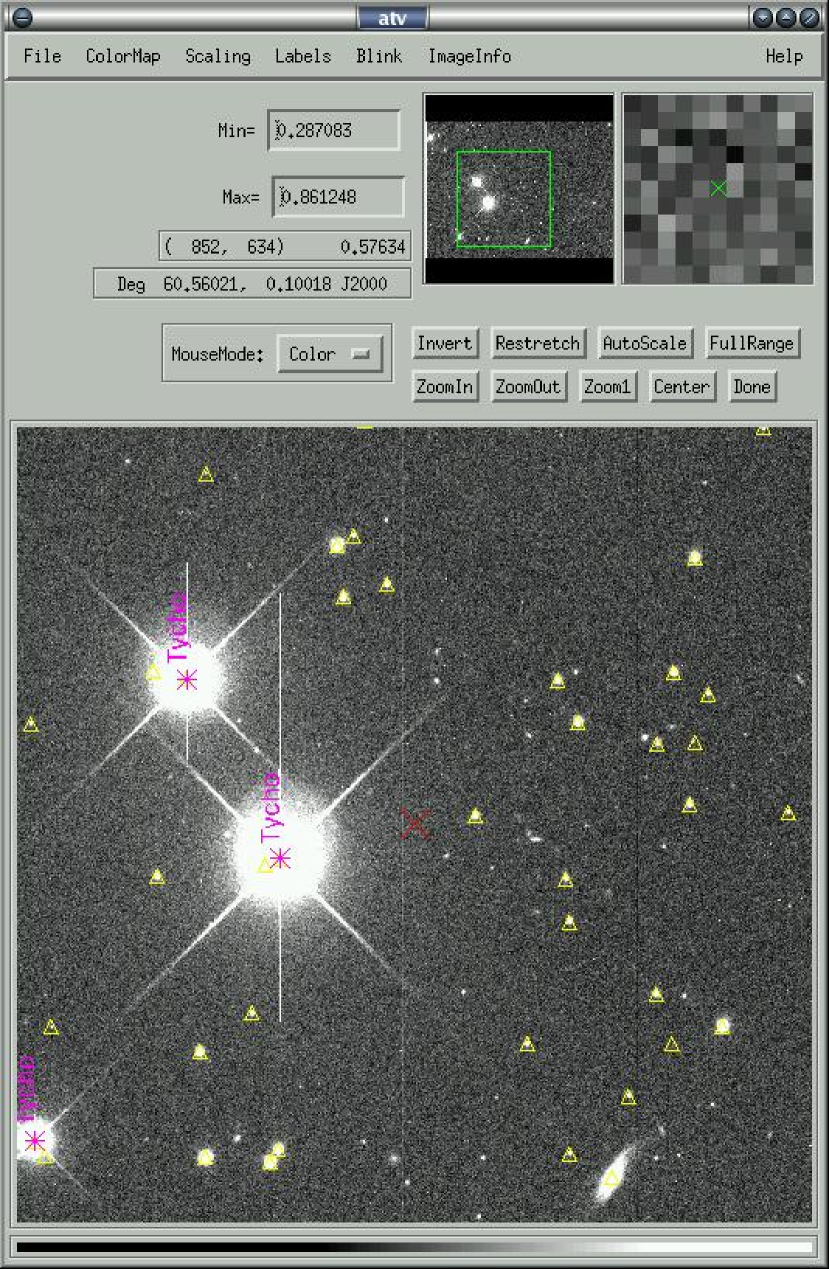
Figure 7: The display tool atvsdss finds a raw SDSS image at the given coordinates, flatfields and calibrates on the fly, matches and overplots Tycho stars (magenta), 2MASS stars (yellow triangles), and displays a red cross at the requested coordinates. See §4.1 for more details.

Using the photoop tools, one can calibrate the raw image data (idR files) at read time, and eliminate the need to store a second, calibrated copy of the image data (Figure 7). Following is a sequence of IDL commands to find the (run,camcol,field) for a position on the sky, read in a calibrated image with astrometric information, match objects in the field to the 2MASS catalog, and display the image with matches overplotted in the IDL display tool atv Barth (2001).

; To see which runs cover RA=60.56, dec=0.1
IDL> imlist=sdss_findimage(60.56,0.1,rerun=137,/print)
           RA           DEC  RUN RERUN CAMCOL FIELD        XPOS        YPOS
------------- ------------- ---- ----- ------ ----- ----------- -----------
     60.56000     0.1000000  211   137      4   131      978.10      177.24
     60.56000     0.1000000  273   137      4   338      917.33      1047.2

; read the first image
file=sdss_name(’idR’,imlist[0].run,imlist[0].camcol,imlist[0].field, filter=’r’)
sdss_readimage,file,image,ivar,/reject_cr,rerun=137,hdr=hdr

; get astrometry and add to header
gsa_approx = sdss_astrom(imlist[0].run,imlist[0].camcol,imlist[0].field, filter=’r’)
gsssputast, hdr, gsa_approx

; display the image in the atv widget which allows panning, zooming,
;  color stretches, etc. and displays WCS coordinates from a FITS
;  header.
atv,image,header=hdr

; Now match 2MASS stars
fobj = tmass_read(60.56, 0.1, 0.2)
astrom_adxy, gsa_approx, fobj.tmass_ra, fobj.tmass_dec, xpix=xpos, ypix=ypos

; and overplot as yellow triangles
atvplot, xpos, ypos, psym=5, symsize=1.5, color=’yellow’

The above commands demonstrate the power of some of the tools available. The atv wrapper atvsdss does all of the above with the simple command

atvsdss, ra=60.56, dec=0.1, /catalog, rerun=137

where the rerun number is required for use of the survey astrom astrometric solutions, and /catalog matches and overplots Tycho stars (magenta), 2MASS stars (yellow triangles), and a red cross at the requested coordinates (Figure 7).

4.2 The Stellar $g-r-i$ color diagram

The following is a simple example that plots the stellar locus in the $g-r-i$ color plane, and provides an introduction to using the catalog data. We start by reading in all the objects from a segment of a run, and then select only the stars with reliable photometry using the object flags. We then demonstrate the conversion of calibrated fluxes into magnitudes, and use these to construct a magnitude-limited sample of stars. Finally, we compute and plot the $g-r$ and $r-i$ colors of these stars. The output of this code is shown in Figure 8.

; Open a plot
dfpsplot, ’gricolor.ps’, /square,/color

; Read in run 273, camcol 3, fields 50-250
; This reads in the data from the ‘‘datasweep’’ trimmed catalogs
objs = sweep_readobj(273, 3, rerun=137, fieldrange=[50,250])

; Select the stars -- sdss_selectobj() removes stars with these bits set:
;  (BLENDED AND NOT NODEBLEND) OR BRIGHT
; see http://www.sdss.org/dr2/products/catalogs/flags.html
; for a thorough discussion
indx = sdss_selectobj(objs, objtype=’star’)
stars = objs[indx]
; Eliminate all saturated stars using flags
; OBJC_FLAGS1, Bit 18 --- Saturated
; OBJC_FLAGS2, Bit 12 --- Interpolated center
; OBJC_FLAGS2, Bit 15 --- PSF Flux Interpolated

; sdss_flagval() returns 2^(flag bit set)
flag1_template = (sdss_flagval(’OBJECT1’,’SATUR’))
flag2_template = (sdss_flagval(’OBJECT2’, ’INTERP_CENTER’)) $
  + (sdss_flagval(’OBJECT2’, ’PSF_FLUX_INTERP’))

; Find all objects with none of these flags set
notset = where(((stars.OBJC_FLAGS AND flag1_template) EQ 0) $
                 AND ((stars.OBJC_FLAGS2 AND flag2_template) EQ 0))
stars = stars[notset]

; Compute the magnitudes, with a flux floor of 1.E-10 nMgy
gmag = 22.5 - 2.5*alog10(stars.psfflux[1] > 1.e-10)
rmag = 22.5 - 2.5*alog10(stars.psfflux[2] > 1.e-10)
imag = 22.5 - 2.5*alog10(stars.psfflux[3] > 1.e-10)

; Pick  stars with r < 19
w = where(rmag LT 19.0)

; Compute g-r and r-i colors
grcolor = gmag[w] - rmag[w]
ricolor = rmag[w] - imag[w]

; Plot the colors
djs_plot, grcolor, ricolor, ps=3, xr=[0,1.8], yr=[0,1.7], $
  charsize=2, xtitle=’g-r’, ytitle=’r-i’, xst=1, yst=1

; Close plot
dfpsclose

4.3 The Proper Motion of a Brown Dwarf

One of the features of these data are the multiple observations of parts of the sky, enabling time domain studies. A particularly simple example is proper motions; Figure 9 shows the position of nearby L6.5 brown dwarf Schneider et al. (2002); Geballe et al. (2002) SDSS J023617.93+004855.0 versus time. This object is in the SDSS Southern Survey equatorial region and has been observed multiple times, both during commissioning observations and during regular survey operations. The RA and DEC offsets with respect to its fiducial position are shown versus time (MJD). The 22 observations span just over five years. The position is taken directly from the pipeline-processed data (for a discussion of SDSS astrometry, see Pier et al. 2003) and clearly show the proper motion of this faint object (140 mas/year in RA, -155 mas/year in DEC). The position errors determined from this fit are 60 mas in each coordinate. Several SDSS brown dwarfs were identified in the commissioning and calibration data (Fan et al.  2000) and a project to measure the proper motions of nearby stars and substellar objects is underway.

The following code fragment creates Figure 9; in particular, it demonstrates the use of sdss_findallobj to find multiple observations of objects in the data. Most observations of this object are not yet public; we include them in the figure to show what will be possible with the complete data set.

;Open the plot
dfpsplot, ’bd.ps’, /color,/square

; This is SDSSJ023617.93+004855.0
ra = 39.0747106
dec = 0.8152421

; Find all the observations of this object in rerun 137
imlist = sdss_findallobj(ra, dec, rerun=137)

; Specify the fields to extract
select_tags = [’RUN’, ’CAMCOL’, ’FIELD’, ’ID’, ’MJD’, $
               ’PSFFLUX*’, $
               ’RA’, ’DEC’, ’OFFSET*’, ’CALIB_STATUS’]

; Read in these fields
objs = sdss_readobjlist(inlist=imlist, select_tags=select_tags, /silent)

; Define time axis
dmjd = objs.mjd - 50000

; Compute the change in RA and DEC in mas
dra = (objs.ra - ra)*3.6d6*cos(dec/!radeg)
ddec = (objs.dec - dec)*3.6d6


; Plot the change in RA with time
djs_plot, dmjd, dra, yr=[-1200,1200], yst=1, charsize=2, $
  thick=3, ps=6, xtitle=’MJD-50000’, ytitle=’\Delta \theta (mas)’
; Plot typical error of 60 mas
errplot, dmjd, dra-60.0, dra+60.0, thick=3

; Plot the change in DEC with time
djs_oplot, dmjd, ddec, thick=3, ps=7, line=2
; Plot error of 60 mas
errplot, dmjd, ddec-60.0, ddec+60.0, thick=3

; Overplot linear fits
oplot,dmjd,poly(dmjd,linfit(dmjd, dra)), thick=3
oplot,dmjd,poly(dmjd,linfit(dmjd, ddec)), thick=3, line=2

; Output a label
djs_xyouts, 1100, 900, ’SDSSJ023617.93+004855.0’, charsize=2.5

; Close the plot
dfpsclose

4.4 Star Formation and Young Stellar Objects

Figure 2 shows a color composite from the three most sensitive SDSS bands (g, r and i) of a region from runs 259/273 centered on the star forming region NGC 2068/NGC 2071/HH24-26. Note the line of Herbig-Haro (HH) objects in the outflow jet. As their emission is dominated by emission lines, HH objects have characteristic colors and can be automatically identified and counted in these regions of high obscuration. We find that there is a very different density distribution of these objects in the Taurus and Orion star-forming regions (Knapp et al., 2004, in preparation).

The spectral energy distributions of the stars in NGC 2068 and NGC 2071 can be constructed from the five SDSS and three 2MASS bands, giving the luminosity function, the frequency of low mass objects and the incidence of circumstellar dust. UV-excess objects, i.e. young T Tauri stars, can be discovered and mapped across the Orion and Taurus star-forming regions (McGehee et al.  2004).

4.5 Structure of the Galactic Halo and Vertical Structure of the Disk

Because of the depth and color discrimination of SDSS photometry, the SDSS data have enabled major contributions to studies of the structure of the Galactic halo Yanny et al. (2000); Ivezić et al. (2000); Odenkirchen et al. (2001); Newberg et al. 2003a . These and other studies of distant halo objects Ibata et al. (1995); Johnston et al. (1995); Majewski et al. (2003); Martínez-Delgado et al. (2004) show the presence of long streams in the halo produced by the tidal disruption of satellite systems (small galaxies and loosely bound globular clusters). The data described herein allow these streams to be traced much closer to the Galactic plane. The SDSS stellar data at low Galactic latitudes can be used to investigate the relationships among the thin disk, the thick disk and the Galactic halo, tracing the metallicity of each component. The discovery of these halo structures, and the ability of SDSS to follow the structure close to the Galactic plane, provide the impetus for a new initiative to use the SDSS hardware and software to map the structure of the Galactic halo and the disk-halo interface, known as SEGUE (Newberg et al. 2003b, , Sloan Extension for Galactic Underpinnings and Evolution).

The vast majority of the red stars detected by SDSS are late-type disk dwarfs and subdwarfs. Hawley et al. (2002, and in prep.) show a well-established color-absolute magnitude relationship for dwarfs of spectral type M0 and later, which allows the vertical mapping of the disk to a distance of about 1 kpc from the Galactic plane, as well as the three-dimensional distribution of the interstellar dust. Measurements at different Galactic latitudes, especially at low latitudes, allow the measurement of the disk scale length and disk scale height for these stars McGehee et al.  in prep ; Jurić et al. (2004).

4.6 Properties of Interstellar Dust

Reddening measured by fitting the position of the “blue tip” of the stellar locus in ($u,g,r,i,z$) color space can be used to investigate possible deviations from the standard extinction law by comparing $E(u-g)$ with $E(g-r)$ in different directions (Finkbeiner et al. 2004). The mosaic images in Figures 2, 3 and 4 demonstrate that the dust clouds also have different emission/reflection properties. In particular, the Taurus dark clouds (Fig. 3) glow at red wavelengths, perhaps due to extended red emission Witt et al. (1998). Differences between the emission properties of dust clouds, and of the illuminating starlight, can be investigated over large areas with these data.

5 Acknowledgments

Partial support for the computer systems required to process, store and distribute these data was provided by NASA via grant NAG5-6734, by NASA’s Hubble Fellow program, and by Princeton University. The NASA funds were originally provided in support of an Associate Investigator Program with WIRE. We thank NASA and the WIRE PI, Perry Hacking, both for the opportunity to work in the WIRE team and for generously permitting us to apply the funding towards support of the Orion data reduction. DPF is a Hubble Fellow supported by HST-HF-00129.01-A. C. Rockosi is a Hubble Fellow supported by HST-HF-01143.01-A. We also thank Princeton University for generous support. This research made use of the IDL Astronomy User’s Library at Goddard Space Flight Center.

This publication makes use of data products from the Two Micron All Sky Survey, which is a joint project of the University of Massachusetts and the Infrared Processing and Analysis Center/California Institute of Technology, funded by the National Aeronautics and Space Administration and the National Science Foundation.

Funding for the SDSS has been provided by the Alfred P. Sloan Foundation, the Participating Institutions, the National Aeronautics and Space Administration, the National Science Foundation, the U.S. Department of Energy, the Japanese Monbukagakusho, and the Max Planck Society. The SDSS Web site is http://www.sdss.org/.

The SDSS is managed by the Astrophysical Research Consortium (ARC) for the Participating Institutions. The Participating Institutions are The University of Chicago, Fermilab, the Institute for Advanced Study, the Japan Participation Group, The Johns Hopkins University, Los Alamos National Laboratory, the Max-Planck-Institute for Astronomy (MPIA), the Max-Planck-Institute for Astrophysics (MPA), New Mexico State University, University of Pittsburgh, Princeton University, the United States Naval Observatory, and the University of Washington.

Appendix A Structure of the calibObj Files

A current description of the calibObj data format is available at the website¹ and is reproduced here for convenience. Fields unchanged from the fpObjc files are not repeated here, and are described in Stoughton et al. (2002).

1. calibObj book-keeping values:

   RUN             LONG      Run number
   RERUN           STRING    Rerun name
   CAMCOL          LONG      Camera column [1..6]
   FIELD           LONG      Field number
   ID              LONG      Object ID, starting at 1 and unique in each field
   PARENT          LONG      ID of parent, -1 if this is a parent object
   NCHILD          LONG      Number of children deblended from this object
   MJD             LONG      Modified Julian Day for date of observation
   TAI             DOUBLE[5] Mean time of observation for the object center
                             in each filter, where TAI = 24 * 3600 * MJD
   AIRMASS         FLOAT[5]  Airmass approximated as csc(zenith-angle)
   PSP_STATUS      LONG[5]   "Status" field from the psField file
   CALIB_STATUS    INT[5]    Status of photometric calibration

2. calibObj calibration parameters:

   NMGYPERCOUNT    FLOAT[5]    Calibration of nano-maggies per count
   NMGYPERCOUNT_IVAR  FLOAT[5] Formal error in the photometric calibration as
                               an inverse variance; =0 if there were no calibration
                               stars and a default calibration was used instead
   CLOUDCAM        INT[5]      Photometricity in each filter:
                                -1=unknown, 0=cloudy, 1=clear
   EXTINCTION      FLOAT[5]    Galactic extinction in magnitudes, defined as
                               [5.155, 3.793, 2.751, 2.086, 1.479] * E(B-V)
                               where E(B-V) is from the SFD98 dust maps.
                               Fluxes (and their errors) can be corrected
                               for Galactic extinction as follows:
                                 Corrected-Flux = Flux * 10^(Extinction/2.5)
   PIXSCALE        FLOAT[5]    Pixel scale [arcsec/pix]
   PSF_FWHM        FLOAT[5]    PSF FWHM [arcsec]
   PHI_OFFSET      FLOAT[5]    Calibration angle [degrees] to add to any
                               uncalibrated position angles such that they mean
                               degrees east of north.

3. calibObj structure calibrated quantities:

   RA              DOUBLE      J2000 RA [deg] in canonical (r-band) filter
   DEC             DOUBLE      Declination [deg] in canonical (r-band) filter
   OFFSETRA        FLOAT[5]    RA of center in this filter relative to RA [arcsec]
   OFFSETDEC       FLOAT[5]    DEC of center in this filter relative to RA [arcs
   PHI_ISO_DEG     FLOAT[5]    Isophotal fit, angle E of N [deg]
   PHI_DEV_DEG     FLOAT[5]    De Vaucouleurs fit, angle E of N [deg]
   PHI_EXP_DEG     FLOAT[5]    Exponential fit, angle E of N [deg]
   SKYFLUX         FLOAT[5]    Sky level [nMgy/arcsec^2]
   SKYFLUX_IVAR    FLOAT[5]
   PSFFLUX         FLOAT[5]    PSF flux [nMgy]
   PSFFLUX_IVAR    FLOAT[5]
   FIBERFLUX       FLOAT[5]    Fiber flux, 3 arcsec diameter [nMgy]
   FIBERFLUX_IVAR  FLOAT[5]
   MODELFLUX       FLOAT[5]    Model flux [nMgy]
   MODELFLUX_IVAR  FLOAT[5]
   PETROFLUX       FLOAT[5]    Petrosian flux [nMgy]
   PETROFLUX_IVAR  FLOAT[5]
   DEVFLUX         FLOAT[5]    De Vaucouleurs flux [nMgy]
   DEVFLUX_IVAR    FLOAT[5]
   EXPFLUX         FLOAT[5]    Exponential flux [nMgy]
   EXPFLUX_IVAR    FLOAT[5]
   APERFLUX        FLOAT[NAPER,5]  Aperture fluxes [nMgy]in radii of size 0.223,
                                   0.670,1.024,1.745,2.972,4.584,7.359,11.306,
                                   18.020,27.922,43.770,68.307,106.73,166.52,
                                   260.37 arcsec; our default is to return
                                   only those fluxes out to 11.3 arcsec,
                                   unless NAPER is explicitly specified
   APERFLUX_IVAR   FLOAT[NAPER,5]

Appendix B Using Inverse Variance

Flux errors are expressed as inverse variance (ivar) in the calibObj files. This is convenient for inverse variance weighting of combined quantities, and handles zero signal/noise (ivar = 0) gracefully, as the following example demonstrates.

B.1 Color Cut

To select all stars with flux ratio $r/i$ greater than some color ratio $c$ with $n\sigma$ confidence, one writes the inequality as $r-ic>n\sigma$, where $\sigma$ is the uncertainty in the quantity $r-ic$, or

$$\sigma=\left(\frac{1}{I_{r}}+\frac{c^{2}}{I_{i}}\right)^{1/2}$$

where $I_{r}$ and $I_{i}$ are the r and i-band inverse variance respectively. Multiplying by $\sqrt{I_{r}I_{i}}$ yields the inequality

$$(r-ic)\sqrt{I_{r}I_{i}}>n\sqrt{I_{i}+c^{2}I_{r}}$$

which concisely expresses the desired condition without a division by any of the parameters, and correctly handles the limiting cases of zero or negative fluxes, or inverse variance equal to zero (non-measurement). The conventional expression of this with magnitudes and $\sigma$ instead of inverse variance requires handling the special cases of zero or negative fluxes in either band, and cannot tolerate zero flux in either band.

Many astronomers will want to work with magnitudes, related to nMgy fluxes by

$$m=22.5-2.5\log_{10}(flux)$$

but will find that any flux and color cuts are most easily performed in flux units. These fluxes and magnitudes are on the natural SDSS system, and are offset from the true AB system by a few hundredths of a magnitude in each band (see Abazajian et al. 2004 for estimated offsets).

B.2 Extinction Corrections

Extinction values are presented in magnitudes for historical reasons. The extinction estimates provided are based on maps of IR dust emission (Schlegel et al. 1998) and are most reliable in the limit of long wavelengths. Extinction values are given in the calibObj files for each SDSS band, assuming a standard interstellar reddening law of $R_{V}=3.1$ in the parameterization of Cardelli, Clayton, & Mathis (1989). Because the SFD98 dust map is calibrated to $E(B-V)$, it is presented as $E(B-V)$ reddening. This has led to the misunderstanding that the presented $E(B-V)$ is valid for all values of $R_{V}$, when in fact it is the the near IR extinction (e.g. SDSS z band) that is roughly constant with changes in $R_{V}$. Therefore, if the dust along a given line of sight is known to have a different value of $R_{V}$, it is necessary to extrapolate the extinction from a red band (e.g. z band) to the desired band using the appropriate reddening law.

The reader is reminded that flux uncertainties must be modified when correcting for extinction. Unlike magnitude uncertainties, which are fractional uncertainties, flux uncertainties are absolute, and must be amplified by the same factor as the flux when extinction correction are applied. To correct flux $F$ and inverse variance $I$ for an extinction of $A$ magnitudes, use:

$$F_{corr}=10^{0.4A}F$$

and

$$I_{corr}=10^{-0.8A}I.$$

Figure 2: Orion: a section of runs 259 and 273 centered at J2000 $(\alpha,\delta)=(05^{h}48^{m}28^{s},+00^{\circ}04^{\prime}48^{\prime\prime}).$ The (R,G,B) color planes represent SDSS (i,r,g) filters respectively, so that H$\alpha$ emission appears green. Celestial North is indicated by the arrow in (d). The widths of panels ($a-d$) are $108^{\prime},54^{\prime},27^{\prime}and13.5^{\prime}$ respectively. Nebulae NGC 2071 (upper) and NGC 2068 are visible in panel ($b$). Panel ($d$) zooms in on the object Herbig-Haro 24 (upper middle).

Figure 3: Taurus: a section of runs 3512 and 3559 centered at $(\alpha,\delta)=(04^{h}24^{m}40^{s},+25^{\circ}41^{\prime}24^{\prime\prime})$. The color scheme and scale are identical to Figure 2. The large dark cloud in the lower right of ($a$) is Barnard 215, which joins with Lynds 1506 further to the right. Panel ($d$) zooms in on Herbig-Haro 31A,B,C,D, and associated outflows (middle left).

Figure 4: Cygnus: a section of runs 4115 and 4119 centered at $(\alpha,\delta)=(20^{h}36^{m}04^{s},+40^{\circ}26^{\prime}24^{\prime\prime})$. The color scheme and scale are identical to Figure 2. The H II region LBN 271 is visible in panel ($a$) (middle left). Panel ($d$) zooms in on a beautiful complex of dark clouds in front of LBN 258.

Figure 6: Histograms of aperture magnitude differences between runs 259 and 297 for the 5 SDSS bands. Stars with $7.43^{\prime\prime}$ radius aperture magnitudes brighter than (19.0,19.0,19.0,18.5,17.0) in (u,g,r,i,z) are shown. Note that the measurement uncertainty in each run is a factor of $\sqrt{2}$ smaller than the histogram width. The bimodality in the g-band is likely caused by $1-2\%$ variation in the flat-fields with time.

Figure 8: A $g-r-i$ color plot showing the stellar locus, based on the stars in 200 fields from camera column 3 of run 273, restricted to stars with apparent magnitude $r<19$. The colors are apparent colors based on PSF fluxes with no correction made for Galactic extinction. The IDL code that generated this figure is in §4.2.

Figure 9: The relative position of the L6.5 brown dwarf SDSSJ023617.93+004855.0 as a function of time. The solid line is a fit to the change in RA (relative to its fiducial position; squares), while the dashed line is a fit to the change in DEC (crosses). The errors in the positions are 60 mas in both coordinates. The 22 SDSS observations clearly show the proper motion of this faint object (140 mas/year in RA, -155 mas/year in DEC). The code that generated this figure is in §4.3.

Table 1: SDSS Galactic Plane Runs

Run	Date	MJD	Strip	Node	Incl	$F_{0}$	$F_{1}$	$A$	$l$	$b$	PSF	Phot
	UT			deg	deg			deg2	deg	deg	′′
(1)	(2)	(3)	(4)	(5)	(6)	(7)	(8)	(9)	(10)	(11)	(12)	(13)
211	1998/10/29	51115	82S	283.22	0.01	11	385	71.2	210.2	-3.3	1.36	Y
250	1998/11/16	51133	82N	62.10	0.02	11	455	84.5	201.9	-18.0	1.55	Y
259	1998/11/17	51134	82N	299.41	0.01	12	567	105.6	206.7	-9.5	1.19	Y
273	1998/11/19	51136	82S	286.54	0.01	11	534	99.6	206.1	-11.1	1.41	N
297	1998/11/22	51139	82O	92.04	0.04	11	203	36.7	206.0	-11.0	1.47	Y
307	1998/11/23	51140	82N	318.93	0.01	11	186	33.4	212.4	0.0	1.21	N
308	1998/11/23	51140	10N	271.30	0.01	11	216	39.1	216.0	4.2	1.24	Y
994	1999/10/06	51457	76S	275.04	15.00	11	133	23.4	209.9	-5.0	1.84	N
1923	2000/12/08	51886	0O	215.00	44.99	29	71	8.2	86.4	0.0	1.75	U
1924	2000/12/08	51886	0O	354.00	45.99	34	78	8.6	168.6	11.9	1.88	U
1925	2000/12/08	51886	0O	349.98	45.78	17	48	6.1	165.3	6.6	1.60	U
2955	2002/02/07	52312	82N	9.82	0.00	21	166	27.7	209.3	-4.5	2.07	Y
2960	2002/02/08	52313	82S	25.79	0.01	11	127	22.2	208.0	-7.4	1.16	Y
2968	2002/02/09	52314	82N	90.64	0.00	19	94	14.4	207.8	-7.3	1.68	Y
3511	2002/12/06	52614	0O	65.19	90.14	14	89	14.4	163.5	-8.2	1.17	Y
3512	2002/12/06	52614	0O	335.41	25.32	11	90	15.2	177.3	-9.3	1.22	Y
3557	2002/12/31	52639	0O	65.50	89.96	11	87	14.6	165.6	-10.5	1.26	Y
3559	2002/12/31	52639	0O	335.41	25.31	11	86	14.4	176.4	-9.9	1.20	Y
3610	2003/01/27	52666	61N	274.99	52.50	17	148	25.1	139.0	-10.8	1.63	Y
3628	2003/01/28	52667	61S	275.01	52.52	17	165	28.3	137.3	-10.9	0.97	Y
3629	2003/01/28	52667	61N	275.00	52.50	11	129	22.6	142.0	-10.9	0.97	Y
3634	2003/01/29	52668	62N	275.00	50.01	18	162	27.5	159.1	-13.0	1.04	Y
3642	2003/02/01	52671	62S	274.99	49.99	11	97	16.5	135.6	-13.2	1.73	Y
3643	2003/02/01	52671	62S	274.99	50.00	11	119	20.7	159.1	-13.2	1.68	Y
4114	2003/09/20	52902	0S	309.49	90.02	41	127	16.5	80.1	0.0	1.59	Y
4115	2003/09/20	52902	0S	309.34	90.15	11	69	11.2	78.7	0.0	1.36	Y
4116	2003/09/20	52902	0O	219.49	41.40	11	77	12.7	82.1	0.0	1.40	Y
4119	2003/09/20	52902	0O	309.40	90.08	11	70	11.4	79.8	0.0	1.71	Y

Note. — Col. (1): SDSS Run number. Col. (2): UT Date. Col. (3): UT MJD. Col. (4): Survey strip number, 82 and 10 are on the Celestial Equator; N=north, S=south, O=other (non-survey strips). Col. (5,6): J2000 node, inclination of stripe great circle. Col. (7): Start field for run – in some cases ramp up takes more than 11 fields. Col. (8): End field. Col. (9): Gross area in square degrees. Col. (10, 11): Galactic $(l,b)$ of closest approach to the Galactic Plane of any field center. Col. (12): Median PSF FWHM (r-band, camera column 3). Col. (13): Photometric? (Y=yes, N=no, U=unkown). Run 273 has an aperture obstruction early in the run, and run 307 is slightly cloudy near the end. Data in the 1998-1999 runs are now public.

Table 2: CVS Products

Product	CVS Version	Language	Analysis?	Description
dust	v0_0	IDL/Fortran/C	Opt	The Schlegel et al. (1998)
				$E(B-V)$ extinction maps
eups	v0_4	Perl	Opt	Product management software
first	v03Apr11	N/A	Opt	The FIRST [4] Radio catalog
idlutils	v5_0_0	IDL/Fortran/C	Yes	General IDL tools; Required for all IDL tasks
photoop	v1_1	Perl/IDL	Yes	SDSS Perl/IDL tools
runList.par	N/A	N/A	Yes	The list of runs processed, and their locations
twomass	allsky	N/A	Opt	The 2-MASS [6]
				Point Source Catalog
tycho2	v0_0	N/A	Opt	The Tycho [13] astrometric catalog
ucac	v2_final	N/A	Opt	The UCAC [41] astrometric
				catalog
usno	vB	N/A	Opt	The USNO-B [27] astrometric
				catalog

Note. — The list of all products used for either processing, analysing or accessing the data. We limit ourselves to those products unique to this reduction; the reader is referred to Stoughton et al. (2002) for the official survey pipeline code. The column “Analysis” marks products either necessary (“Yes”) or optional (“Opt”) for data analysis.

References

- Abazajian et al. [2003] Abazajian, K., Adelman-McCarthy, J. K., Agüeros, M. A., et al. 2003, AJ, 126, 2081 (DR1)
- Abazajian et al. [2004] Abazajian, K., Adelman-McCarthy, J. K., Agüeros, M. A., et al. 2004, AJ in press (DR2)
- Barth [2001] Barth, A. J. 2001, in ASP Conf. Ser., Vol. 238, Astronomical Data Analysis Software and Systems X, eds. F. R. Harnden, Jr., F. A. Primini, & H. E. Payne (San Francisco: ASP), 385
- Becker et al. [1995] Becker, R.H., White, R.L., Helfand, D.J. 1995, ApJ, 450, 559
- Cardelli, Clayton & Mathis [1989] Cardelli, J. A., Clayton, G. C., & Mathis, J. S. 1989, ApJ, 345, 245
- Cutri et al. [2003] Cutri, R. M., et al. 2003, Explanatory Supplement to the 2MASS All Sky Data Release (Pasadena: Caltech) and VizieR Online Data Catalog, 2246
- Fan et al. [2000] Fan, X., Knapp, G., Strauss, M. A., et al. 2000, AJ, 119, 928
- Finkbeiner et al. [2004] Finkbeiner, D. P. et al. 2004, in prep.
- Fukugita et al. [1996] Fukugita, M., Ichikawa, T., Gunn, J.E., Doi, M., Shimasaku, K., & Schneider, D.P. 1996, AJ, 111, 1748
- Geballe et al. [2002] Geballe, T.R., Knapp, G.R., Leggett, S.K., et al. 2002, ApJ, 564, 466
- Gunn et al. [1998] Gunn, J.E., Carr, M., Rockosi, C.M., Sekiguchi, M., et al. 1998, AJ, 116, 3040
- Hawley et al. [2002] Hawley, S.L., Covey, K.R., Knapp, G.R., et al. 2002, AJ, 123, 3409
- Høg et al. [2000] Høg, E., Fabricius, C., Makarov, V.V., et al. 2000, A&A, 355, L27
- Hogg et al. [2001] Hogg, D. W., Finkbeiner, D. P., Schlegel, D. J. & Gunn, J. E. 2001, AJ, 122, 2129
- Ibata et al. [1995] Ibata, R.A., Gilmore, G., & Irwin, M.J. 1995, MNRAS, 277, 781
- Ivezić et al. [2000] Ivezić, Ž., Goldston, J., Finlator, K., et al. 2000, AJ, 120, 963
- Johnston et al. [1995] Johnston, K.V., Spergel, D.N., & Hernquist, L. 1995, ApJ, 451, 598
- Jurić et al. [2004] Jurić, M., Ivezić, Ž., et al. 2004, in prep.
- Kniazev et al. [2003] Kniazev, A. Y., Grebel, E. K., Hao, L., Strauss, M. A., Brinkmann, J., & Fukugita, M. 2003, ApJ, 593, L73
- Lupton et al. [1999] Lupton, R.H., Gunn, J.E., & Szalay, A.S. 1999, AJ, 118, 1406
- Lupton et al. [2001] Lupton, R.H., Gunn, J.E., Ivezić, Ž., Knapp, G.R., Kent, S.M., & Yasuda, N. 2001, ADASS X, ed. F.R. Harnden, F.A. Primini, & H.E. Payne, ASP Conf. Proc. 238, 269
- Lupton et al. [2003] Lupton, R.H., Ivezić, Ž., Gunn, J.E., Knapp, G.R., Strauss, M.A., & Yasuda, N. 2003, Proc. SPIE, 4836, 350
- Majewski et al. [2003] Majewski, S., Skrutskie, M.F., Weinberg, M.D., & Ostheimer, J.C. 2003, ApJ, 599, 1082
- Martínez-Delgado et al. [2004] Martínez-Delgado, D., Gómez-Flechoso., M., Aparacio, A., & Carrera, R. 2004, ApJ, 601, 242
- [25] McGehee, P. et al. 2004, in preparation
- [26] McGehee, P.M., Anderson, K.S.J., Hobbs, L.M., & York, D.G., in preparation
- Monet et al. [2003] Monet, D.G, Levine, S.E., Canzian, B., et al. 2003, AJ, 125, 984
- [28] Newberg, H.J., Yanny, B., Grebel, E., et al. 2003a, ApJ, 596, L191
- [29] Newberg, H.J., & SDSS Collaboration 2003b, AAS, 203, 112.11
- Odenkirchen et al. [2001] Odenkirchen, M., Grebel, E., Rockosi, C., et al. 2001, ApJ, 548, L165
- Oke & Gunn [1983] Oke, J. B. & Gunn, J. E. 1983, ApJ, 266, 713
- Pier et al. [2003] Pier, J.R., Munn, J.A., Hindsley, R.B., Hennessy, G.S., Kent, S.M., Lupton, R.H., & Ivezić, Ž. 2003, AJ, 125, 1559
- Schlegel et al. [2004] Schlegel, D. J. et al. 2004, in prep.
- Schlegel, Finkbeiner & Davis [1998] Schlegel, D. J., Finkbeiner, D. P., & Davis M. 1998, ApJ, 500, 525 (SFD98)
- Schneider et al. [2002] Schneider, D.P., Knapp, G.R., Hawley, S.L., et al. 2002, AJ, 123, 458
- Smith et al. [2002] Smith, J.A., Tucker, D.L., Kent, S.M., et al. 2002, AJ, 123, 2121
- Stoughton et al. [2002] Stoughton, C., Lupton, R.H., Bernardi, M., et al. 2002, AJ, 123, 485 (EDR)
- Witt et al. [1998] Witt, A.N., Gordon, K.D., & Furton, D.G. 1998, ApJ, 501, L111
- Yanny et al. [2000] Yanny, B., Newberg, H.J., Kent, S., et al. 2000, ApJ, 540, 825
- York et al. [2000] York, D.G., Adelman, J., Anderson, J., et al. 2000, AJ, 120, 1579
- Zacharias et al. [2000] Zacharias, N., Rafferty, T.J., Zacharias, M.I. 2000, ADASS IX, ed. N. Manset, C. Veillet, and D. Crabtree, ASP Conf. Ser. 216, 427