The spin of accreting stars: dependence on
magnetic coupling to the disc

Abstract

We formulate a general, steady-state model for the torque on a magnetized star from a surrounding accretion disc. For the first time, we include the opening of dipolar magnetic field lines due to the differential rotation between the star and disc, so the magnetic topology then depends on the strength of the magnetic coupling to the disc. This coupling is determined by the effective slip rate of magnetic field lines that penetrate the diffusive disc. Stronger coupling (i.e., lower slip rate) leads to a more open topology and thus to a weaker magnetic torque on the star from the disc. In the expected strong coupling regime, we find that the spin-down torque on the star is more than an order of magnitude smaller than calculated by previous models. We also use our general approach to examine the equilibrium (‘disc-locked’) state, in which the net torque on the star is zero. In this state, we show that the stellar spin rate is roughly an order of magnitude faster than predicted by previous models. This challenges the idea that slowly-rotating, accreting protostars are disc locked. Furthermore, when the field is sufficiently open (e.g., for mass accretion rates $\ga 5\times 10^{-9}M_{\odot}$ yr^-1, for typical accreting protostars), the star will receive no magnetic spin-down torque from the disc at all. We therefore conclude that protostars must experience a spin-down torque from a source that has not yet been considered in the star-disc torque models—possibly from a stellar wind along the open field lines.

1 Introduction

Accretion discs are responsible for some of the most energetic and spectacular phenomena in many classes of astrophysical objects, including protostars, white dwarfs (cataclysmic variables and intermediate polars), neutron stars (binary X-ray pulsars), and black holes (both stellar mass X-ray transients and supermassive active galactic nuclei). Gravitational potential energy liberated by the accretion process gives rise to exceptional luminosity excesses and can drive powerful jets and outflows. Accretion onto the central object can occur only as quickly as angular momentum can be transported away from the system. Furthermore, the accretion of disc material, which has high specific angular momentum, spins up the central object, if the object rotates at less than the break-up rate. It is therefore surprising that the central objects (hereafter ‘stars’) are often observed to spin far below their break-up rates, in spite of long-lived accretion. Why does this happen?

There is good evidence that accretion onto magnetized stars occurs along closed magnetospheric field lines that connect the star to the inner edge of the disc. For instance, theoretical models of this sort have been successful in explaining numerous observed features in accreting protostars (e.g., Hayashi et al., 1996; Goodson et al., 1999; Muzerolle et al., 2001), intermediate polars (e.g., Patterson, 1994), and X-ray pulsars (e.g., Joss & Rappaport, 1984; Aly & Kuijpers, 1990; Kato et al., 2001; Kato et al., 2004). In some cases, there is even direct evidence that the stars are magnetized, namely for accreting protostars (Johns-Krull et al., 1999), intermediate polars (Piirola et al., 1993), and X-ray pulsars (Makishima et al., 1999).

Magnetic fields can also be effective at transferring angular momentum away from the star, possibly explaining the observed rotation rates. Torques on the star that are exerted by magnetic field lines anchored to the star and that are also connected to the disc have been calculated by several authors (e.g., Ghosh & Lamb, 1979; Cameron & Campbell, 1993; Lovelace et al., 1995; Wang, 1995; Yi, 1995; Armitage & Clarke, 1996, hereafter AC96; Rappaport et al., 2004). Under certain circumstances, this torque can counteract the angular momentum deposited by accretion, leading to a net spin-down of the star (possibly explaining spin-down episodes observed in X-ray pulsars; Ghosh & Lamb, 1978; Lovelace et al., 1995) or giving rise to an equilibrium state, in which the net torque on the star is zero (possibly explaining the slow spin of some accreting protostars; Königl, 1991, hereafter K91). In this equilibrium state, the spin rate of the central object depends on the accretion rate in the disc, and so a system is then considered to be ‘disc locked.’ Since these models for the magnetic star-disc interaction show that accreting stars can spin more slowly than the break-up rate, there is a general perception that the presence of an accretion disc in any system leads to slow rotation rates. This idea of disc locking has been applied to a variety of problems. As an example, in systems where the moment of inertia of the star is changing (e.g., during contraction), some authors have assumed that disc-locking keeps the star at a constant spin rate (e.g., as applied to protostars by Bouvier et al., 1997; Sills et al., 2000; Barnes et al., 2001; Tinker et al., 2002; Rebull et al., 2004; and suggested for stellar collision products by Leonard & Livio, 1995; Sills et al., 2001; De Marco et al., 2004).

There is a nagging problem with this physical picture, however, because the magnetic torque calculations discussed above (with the exception of Lovelace et al., 1995) assume that the stellar magnetic field remains largely closed and that field lines connect to a large portion of the disc. This assumption is questionable because closed magnetic structures tend to open when enough energy is added to them, and these systems possess a natural source of energy in the form of gravitational potential energy that is released during disc accretion. This energy release can drive outflows and twist field lines, thereby adding energy to the magnetic field. Thus, the general surplus of energy in accreting systems suggests that associated magnetic fields should be dominated by open, rather than closed, topologies. How are low spin rates achieved in this case?

In this paper, we generalize the star-disc interaction model to include the effect of varying field topology (i.e., connectedness). We consider the mechanical energy that is added to the field via differential rotation between the star and disc as the only mechanism responsible for opening the field (though our formulation is easily adaptable for other mechanisms). The time-dependent behavior of a dipole stellar field attached to a rotating, conducting disc has been studied, using an analytic approach, by several authors (e.g., Lynden-Bell & Boily, 1994; Agapitou & Papaloizou, 2000; Uzdensky et al., 2002a, hereafter UKL). They have shown that, as the differential twist angle between the star and disc $\Delta\Phi$ monotonically increases, the torque exerted by field lines first reaches a maximum value, then decreases. This occurs because azimuthal twisting of the dipole field lines generates an azimuthal component to the field, and the magnetic pressure associated with this component acts to inflate the field, which then balloons outward at an angle of $\sim 60^{\circ}$ from the rotation axis, causally disconnecting the star and disc (see also Aly, 1985; Aly & Kuijpers, 1990; Newman et al., 1992; Lovelace et al., 1995; Bardou & Heyvaerts, 1996). Typically, this inflation or opening of the field occurs when a critical differential rotation angle of $\Delta\Phi_{\rm c}\approx\pi$ has been reached, and the amount of flux that opens depends on the strength of the magnetic coupling of the field to the disc (UKL). This analytic work on the field opening has been corroborated by time-dependent, numerical magnetohydrodynamic simulations of the stellar dipole-disc interaction (Hayashi et al., 1996; Goodson et al., 1997, 1999; Miller & Stone, 1997; Kato et al., 2001; Kato et al., 2004; Matt et al., 2002; Romanova et al., 2002; Küker et al., 2003).

Our primary goal in this paper is to determine the effect of the topology of the magnetic field on the torques in the steady-state, star-disc interaction model. In a previous paper (Matt & Pudritz, 2004), we gave a brief outline of this theory and showed that a more open (i.e., less connected) field topology results in a spin-down torque on the star that is less than for the closed field assumption. Consequently, the equilibrium state (with a net zero torque) features a faster spin than predicted by previous models, which calls into question the general belief that accretion discs necessarily lead to slow rotation. The present paper contains a more detailed presentation of the theory and our assumptions, and we consider all possible spin states of the system (not just the equilibrium state). We also extend our analysis to show that there are at least three different modes in which a magnetic star-disc system can operate. Our analysis is applicable to all classes of magnetized objects that accrete from Keplerian discs. However, since an abundance of observational data exists for accreting protostars, in particular for classical T Tauri stars (CTTS’s), we adopt a set of fiducial parameters that are appropriate for these systems and discuss various aspects of the model in this context.

Section 2 contains a formulation of the general model. The special case of a disc locked system is the topic of section 3. The final section (§4) contains a summary of our results and includes a list of problems with using the disc-locking scenario to explain CTTS spins, plus a discussion of three possible configurations of the general system.

2 Star-disc interaction model

Magnetic, star-disc interaction models in the literature differ in their various assumptions, adopted parameter values, and in the introduction of ‘fudge factors,’ but they are quite similar on the whole (for a review, see Uzdensky, 2004). We formulate a general model that builds upon this previous work (mostly following AC96), by including the effect of varying magnetic field topology, via the introduction of the physical parameters $\beta$ and $\gamma_{\rm c}$ (defined below).

According to the usual model assumptions, a rotating star is surrounded by a thin, Keplerian accretion disc. The angular momentum vector of the disc is aligned with that of the star, which rotates as a solid body and at a rate that is some fraction of break-up speed, defined by

$$f\equiv\Omega_{*}\sqrt{{R_{*}^{3}}\over{GM_{*}}},$$ (1)

where $\Omega_{*}$, $R_{*}$, and $M_{*}$ are the angular rotation rate, radius, and mass of the star, respectively. Note that $f$ is always within the range from zero to one. The disc rotates at a different angular rate than the star at all radii, except at the singular corotation radius given by

$$R_{\rm co}=f^{-{2/3}}R_{*}.$$ (2)

For $r<R_{\rm co}$, the disc rotates faster than the star, while for $r>R_{\rm co}$, the angular rotation rate of the star is greater than that of the disc.

The disc is assumed to be in a steady-state wherein the mass accretion rate $\dot{M}_{\rm a}$ is constant in time and at all radii. In a real disc from which winds are launched, $\dot{M}_{\rm a}$ may have a weak radial dependence, but we assume this has a negligible effect on the model. A rotation-axis-aligned dipole magnetic field, anchored into the stellar surface, also connects to the disc. The field is strong enough to truncate the disc at some inner location $R_{\rm t}$ from where disc material is subsequently channeled along magnetic field lines as it accretes onto the star. In general, the disc may have its own magnetic field (either generated in a disc dynamo or carried in by the disc from larger scales). We do not specifically include this field in the model, though it may be responsible for angular momentum transport in the disc (providing $\dot{M}_{\rm a}$) and may also aid in the connection of the stellar field to the disc. Within the disc, the kinetic energy of the gas is much greater than the magnetic energy of the stellar field, but the region above the star and disc (the corona) is filled with low density material, and so the corona is magnetically dominated.

In this configuration, the magnetic field connects the star and disc by conveying torques between the two. Torques are conveyed on an Alfvén wave crossing time, which is much shorter than the Keplerian orbital time. Everywhere that the magnetic field connects the star to the disc, exept at $R_{\rm co}$, the magnetic field is twisted azimuthally by differential rotation between the two. Inside $R_{\rm co}$ the field is twisted such that field lines ‘lead’ the stellar rotation, so torques from field lines threading the region $r<R_{\rm co}$ act to spin up the star (and spin down the disc). Conversely, torques from field lines threading $r>R_{\rm co}$ act to spin the star down (and spin the disc up). The accretion of disc matter onto the star also deposits angular momentum onto the star.

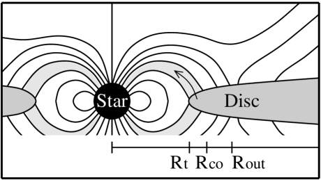
Figure 1: Magnetic star-disc interaction. The stellar field connects to a region of the disc, from $R_{\rm t}$ to $R_{\rm out}$, reaching beyond $R_{\rm co}$ in this case. The stellar field dominates the accretion flow onto the star (arrow).

In order for disc material to accrete, $R_{\rm t}$ must be less than $R_{\rm co}$ so that accreting material loses angular momentum to the star as it falls inward. In order for the star with $f\leq 1$ to feel any spin down torques from the disc, the stellar field must connect to the disc beyond $R_{\rm co}$. Under this condition, the field that connects outside $R_{\rm co}$ transfers angular momentum from the star to the disc. To maintain a steady accretion rate, the disc must then transport this excess angular momentum outward, resulting in an altered disc structure (Sunyaev & Shakura, 1977a, b; Spruit & Taam, 1993; Rappaport et al., 2004). We will define $R_{\rm out}$ as the outermost radial extent of the magnetic connection, and the usual assumption is that $R_{\rm out}\gg R_{\rm co}$. Figure 1 illustrates the basic picture, and shows the locations of $R_{\rm t}$, $R_{\rm co}$, and $R_{\rm out}$ for a possible configuration of the star-disc interaction model.

The assumption of a dipole field refers to the poloidal component of the field, $B_{\rm p}=(B_{r}^{2}+B_{z}^{2})^{1/2}$, where $B_{r}$ and $B_{z}$ are the cylindrical $r$ and $z$ components of the magnetic field, and the closed field only exists in the region interior to $R_{\rm out}$. The dipole field is used for simplicity and because it has the weakest radial dependence ($B_{z}\propto r^{-3}$ along the equator) of any natural magnetic multipole. In reality, the twisting of dipole field lines alters the poloidal field, but this perturbation should be slight in the region where the magnetic field remains closed (as justified by the work cited in §1, e.g., UKL, and see also Livio & Pringle, 1992).

For discussion throughout this paper, it is often instructive to use physical units, especially for comparison with observations. For this purpose, we adopt a set of observationally determined ‘fiducial parameters’ that are appropriate for CTTS’s (e.g., see Johns-Krull & Gafford, 2002):

$$\dot{M}_{\rm a} = 5\times 10^{-8}\;M_{\odot}\;{\rm yr}^{-1},$$

$$M_{*} = 0.5\;M_{\odot},$$

$$R_{*} = 2\;R_{\odot},$$

$$B_{*} = 2\times 10^{3}\;{\rm G},$$

where $B_{*}$ is the stellar magnetic field strength at the equator. However, our formulation of the problem is applicable to any magnetic star-disc system.

2.1 Twisting and slipping of magnetic field lines

The torque exerted by magnetic field lines threading an annulus of the disc of radial width $dr$ is given by (e.g., AC96)

$$d\tau_{\rm m}=-\gamma{\mu^{2}\over r^{4}}dr,$$ (3)

where

$$\gamma\equiv B_{\phi}/B_{z}.$$ (4)

Here, $\mu$ is the dipole moment and $B_{\phi}$ is the azimuthal component of the magnetic field. The radial component, $B_{r}$, is assumed to be negligible within the disc, the torque has been vertically integrated through the disc, and $B_{\phi}$ refers to the value at the disc surface. Here, and throughout this paper, we choose the sign of the torque to be relative to the star such that a positive torque spins the star up, and consequently spins the disc down (and vice versa for a negative torque).

The differential magnetic torque of equation 3 depends not only on $\mu$, but also $\gamma$, which is the ‘twist,’ or pitch angle, of the field. The total (integrated) magnetic torque will also depend on the size and radial location of the magnetically connected region in the disc. While $\mu$ is a constant parameter of the system, the radial dependence of $\gamma$ depends on the physical coupling of the magnetic field to the disc.

In general, the coupling is not perfect. Magnetic forces act to resist the twisting of the field, and so the field will ‘slip’ backward through the disc at some rate $v_{\rm d}$ proportional to $\gamma$. The exact slipping rate depends upon which physical mechanism is at work. In the literature, there are generally three mechanisms discussed (e.g., see Wang, 1995): 1) magnetic reconnection in the disc, 2) reconnection outside the disc, and 3) turbulent diffusion of the magnetic field through the disc. We adopt the latter mechanism, but we further discuss the other two, below.

The magnetic field slips azimuthally at a speed (e.g., Lovelace et al., 1995; UKL)

$$v_{\rm d}={\eta_{\rm t}\over h}\gamma=\beta v_{\rm k}\gamma,$$ (5)

where $\eta_{\rm t}$ is the turbulent magnetic diffusivity, $h$ is the local disc scale height, $v_{\rm k}$ is the Keplerian orbital speed, and we have introduced the dimensionless ‘diffusion parameter’ $\beta\equiv\eta_{\rm t}(hv_{\rm k})^{-1}$. The variable $\beta$ simply parametrizes the coupling of the stellar magnetic field to the disc such that $\beta\gg 1$ corresponds to weak coupling, and $\beta\ll 1$ to strong coupling.

Generally, $\beta$ is a scale factor that compares $v_{\rm d}$ to $v_{\rm k}$, and we have chosen this generic formulation so that the system behavior is largely independent of any particular disc model—as long as the disc obeys Keplerian rotation and provides a steady accretion rate. However, if we temporarily consider a standard $\alpha$-disc (Shakura & Sunyaev, 1973), we may rewrite our diffusivity parameter $\beta$ in a more physically revealing way:

$$\beta={\alpha\over P_{\rm t}}{h\over r},$$ (6)

where $\alpha$ has its usual meaning and $P_{\rm t}$ is the turbulent Prandtl number, equal to the turbulent viscosity divided by $\eta_{\rm t}$. The disc turbulence is likely to be driven by the magneto-rotational instability (MRI; Balbus & Hawley, 1991), which follows the general behavior of an $\alpha$-disc. Since both $\alpha$ and $h/r$ typically have weak radial dependences, and the value of $P_{\rm t}$ is unknown, we assume that $\beta$ is constant in the region of the disc connected to the stellar field.

The value of $\beta$ is not well constrained (AC96 used $\beta=1$), but extreme $\alpha$-disc parameters give an upper limit of $\beta\leq 1$. For a more reasonable estimate, note that a thin disc usually means $h/r\la 0.1$, and $\alpha$ is typically in the range of 0.001 to 0.1 (Sano et al., 2004). So, assuming $P_{\rm t}$ is of order unity, $\beta\la 10^{-2}$. We get a similar estimate using equation 5 and reasonable guesses for CTTS disc parameters,

$$\beta\approx 10^{-2}\left({{\eta_{\rm t}\over 10^{16}\;{\rm cm}^{2}\;{\rm s}^{-1}}}\right)\left({{h\over R_{\odot}}}\right)^{-1}\left({{v_{\rm k}\over 100\;{\rm km}\;{\rm s}^{-1}}}\right)^{-1}.$$ (7)

However, given the uncertainties and possible variation among different systems, and to assess the effect of the coupling of the field to the disc, we retain $\beta$ as a free parameter.

Figure 2: The magnetic twist ($\gamma\equiv B_{\phi}/B_{z}$) times the diffusion parameter $\beta$, as a function of radius along the surface of the disc (thick, solid line). The dotted lines indicate critical radii for a field-opening twist of $\gamma_{\rm c}=\pm 0.5/\beta$ (chosen for illustrative purposes). The locations of $R_{\rm in}$, $R_{\rm co}$, and $R_{\rm out}$ are where $\gamma$ equals $-\gamma_{\rm c}$, 0, and $\gamma_{\rm c}$, respectively.

In the disc connected region, if $v_{\rm d}$ is anywhere less (greater) than the local differential rotation speed between the star and disc, $\gamma$ will increase (decrease) on an orbital time-scale. Thus the magnetic field will quickly achieve a steady-state configuration in which $v_{\rm d}$ equals the local differential rotation rate (e.g., UKL), which gives

$$\gamma=\beta^{-1}\left[{(r/R_{\rm co})^{3/2}-1}\right].$$ (8)

The solid line in Figure 2 shows the quantity $\beta\gamma$ as a function of radius (normalized to $R_{\rm co}$) along the surface of the disc. The magnetic twist is zero at $R_{\rm co}$, and is oppositely directed on either side of $R_{\rm co}$. Also, at a given radius, the twist will be larger for smaller values of $\beta$ (and vice versa).

We have assumed that the field coupling is determined by turbulent diffusion, and when $\beta$ is constant, we find that $\gamma\propto r^{1.5}$ (eq. 8, for $r\gg R_{\rm co}$). Other coupling mechanisms (as discussed above) result in a different radial dependence of $\gamma$. For example, Wang (1995) showed that if the twist is limited by reconnection in the disc, $\gamma\propto r^{1.6}$ (for $r\gg R_{\rm co}$), while for reconnection outside the disc, $\gamma$ approaches a constant value (for $r\gg R_{\rm co}$). On the other hand, Livio & Pringle (1992) and AC96, assumed $\gamma$ was limited by reconnection in the stellar corona, and they used the same formulation as equation 8 (with $\beta=1$). In any case, note that the radial dependence of the differential magnetic torque is dominated by the falloff of the dipole magnetic field (which results in the $r^{-4}$ dependence of eq. 3). Therefore, the choice of magnetic coupling mechansim will not much influence our results (AC96). Similarly, a small radial dependence of $\beta$ (which we take as constant) will not introduce a large error.

2.1.1 Maximum twist for dipole field

As discussed in section 1, several authors have shown that dipole field lines will transition from a closed to an open topology when a critical differential rotation angle of $\Delta\Phi_{\rm c}\approx\pi$ has been reached. This corresponds to a critical field twist of $\gamma_{\rm c}\approx 1$. Since the twisting of field lines does not significantly alter the poloidal configuration of the field lines that remain closed, and as an approximation, we will assume that the opening of field lines is only important for the determination of the size of the connected region (i.e., to determine $R_{\rm out}$). Thus, we include the effect of field line opening in the steady-state torque theory in the following manner: we will use equation 8 only where $\gamma<\gamma_{\rm c}$ and assume that the field will be open everywhere else (a similar approach was used by Lovelace et al., 1995 and justified by the work of UKL). In other words, wherever equation 8 predicts $\gamma\geq\gamma_{\rm c}$, the magnetic connection is assumed to be severed, so the star and disc are causally diconnected, such that no torques can be conveyed between the two. The size of the connected region in a Keplerian disc is then limited to a finite radial extent near $R_{\rm co}$, where the differential rotation between the star and disc is the smallest.

Will field lines, once opened by differential rotation, remain open? It has been suggested that such field lines could reconnect in the current sheet formed during the opening (Aly & Kuijpers, 1990; Uzdensky et al., 2002b). In order for this to be important, the time-scale for reconnection should be comparable to or shorter than that for field line opening. It is not clear whether this is the case in these systems (Uzdensky et al., 2002b; Matt et al., 2002), but even if it is, there are other considerations. First, due to the topology of the field, reconnection must initially occur between open field lines at the smallest radii (connecting to the lowest latitude on the star). It is possible that, if reconnection does occur, only a small amount of flux will be able to reconnect before this newly connected field again begins to open (as in the simulations of Goodson et al., 1999, and see Uzdensky et al., 2002b). In this case, the size of the connected region (in a time-averaged sense) will be only slightly larger than if the reconnection were never to occur. Second, the configuration of the opened field is favorable to launch magnetocentrifugal flows from the disc (Blandford & Payne, 1982). We ignore such outflows in our model, but in a real system, they could help to maintain an open magnetic field configuration. Thus we conclude that, once the field has opened, reconnection along the current sheet is unlikely to significantly affect the size of the connected region.

2.1.2 Maximal spin-down torque for maximal twist

It is instructive to look at the maximum possible spin-down torque in this system. Regardless of any disc model or any magnetic coupling physics, the largest possible magnetic torque on a star that connects to a disc via a dipole magnetic field occurs when the field is maximally twisted ($\gamma=\gamma_{\rm c}$) at all radii along the surface of the disc. Spin-down torques on the star only occur along field lines threading the disc outside $R_{\rm co}$. Also, the accretion of mass from a Keplerian disc always adds angular momentum to the star. Therefore, the largest net spin-down torque on the star occurs when the disc is truncated exactly at the corotation radius ($R_{\rm t}=R_{\rm co}$), the field threads the disc to $R_{\rm out}\rightarrow\infty$, and the disc does not accrete ($\dot{M}_{\rm a}=0$). One then integrates equation 3 from $R_{\rm co}$ to $\infty$ to get

$$\tau^{\rm max}_{\rm twist}=-{\gamma_{\rm c}\over 3}{\mu^{2}\over R_{\rm co}^{3}}.$$ (9)

This is the absolute maximum spin-down torque that a star can undergo from a disc that exists in the equatorial plane and to which the star is connected via a dipole magnetic field. It is even independent of the rotation profile of the disc, except that angular rotation rate of the disc is slower than the star outside some radius $R_{\rm co}$. It is also independent of the angular momentum transport mechanism within the disc.

To achieve this maximal torque requires that a) the field twist has no radial dependence and b) the twist is very nearly equal to the maximum allowed value of $\gamma_{\rm c}$. If the coupling of the field to a Keplerian disc is determined by turbulent diffusion, a constant $\gamma$ can only be achieved in the unlikely event that $\eta_{\rm t}$ decreases with radius to exactly counteract the increase in differential rotation rate. Alternatively, reconnection in the stellar or disc corona may also lead to a constant $\gamma$ (Aly & Kuijpers, 1990; Wang, 1995, but see discussion in §2.1.1). However, in either case, it is not clear why the value of the constant twist would necessarily be near the maximal value $\gamma_{\rm c}$ (instead of, e.g., $0.1\gamma_{\rm c}$). Though this torque may not be very realistic, it is similar in strength to the spin-down torque used in previous models (e.g., it is the equivalent to the solution of AC96, for $\gamma_{\rm c}=1$).

2.1.3 Determination of $R_{\rm in}$ and $R_{\rm out}$

To derive a more realistic magnetic torque, we adopt equation 8 for the radial dependence of $\gamma$. Following Lovelace et al. (1995), we assume that this equation is only valid where $|\gamma|\leq\gamma_{\rm c}$, and that the field is open everywhere else. Thus, equation 8 predicts that the outer radius of the magnetically connected region in the disc is

$$R_{\rm out}=(1+\beta\gamma_{\rm c})^{2/3}R_{\rm co}.$$ (10)

There is a corresponding location insided $R_{\rm co}$ at which the twist formally exceeds the critical value, given by

$$R_{\rm in}=(1-\beta\gamma_{\rm c})^{2/3}R_{\rm co}.$$ (11)

The dotted lines in Figure 2 indicate these radii for $\beta\gamma_{\rm c}=0.5$, in which case $R_{\rm in}\approx 0.63R_{\rm co}$ and $R_{\rm out}\approx 1.31R_{\rm co}$. It is evident that the field topology is a function of $\beta\gamma_{\rm c}$ such that more diffusion in the disc allows for a larger connected region. Note that, if $\beta\gamma_{\rm c}\geq 1$, the field can remain connected to the disc at any $r<R_{\rm co}$ (since $R_{\rm in}$ is then not defined).

The typical assumption of a closed magnetic topology, corresponding to $R_{\rm out}\rightarrow\infty$ (e.g., AC96; Yi, 1995), is equivalent to $\gamma_{\rm c}\rightarrow\infty$—the field is allowed to twist to arbitrarily large values without opening. In order to consider the effect of varying topology (i.e., where the field is open beyond some finite $R_{\rm out}$), we adopt a value of $\gamma_{\rm c}=1$ (as justified by, e.g., UKL). However, we will retain $\gamma_{\rm c}$ as a parameter in all of our formulae for a comparison between the two cases ($\gamma_{\rm c}\rightarrow\infty$ and $\gamma_{\rm c}=1$) and so that different values of $\gamma_{\rm c}$ may be considered by the reader. The combined parameter $\beta\gamma_{\rm c}$ appears throughout our formulation. We generally think of this parameter in two ways. First, when $\gamma_{\rm c}=\infty$, the stellar field is closed and connects to the entire disc, and this represents the ‘standard’ star-disc interaction model. Second, for the more realistic case of $\gamma_{\rm c}=1$, the field topology is partially open, and $R_{\rm out}$ then depends on $\beta$.

2.2 Three possible states of the system

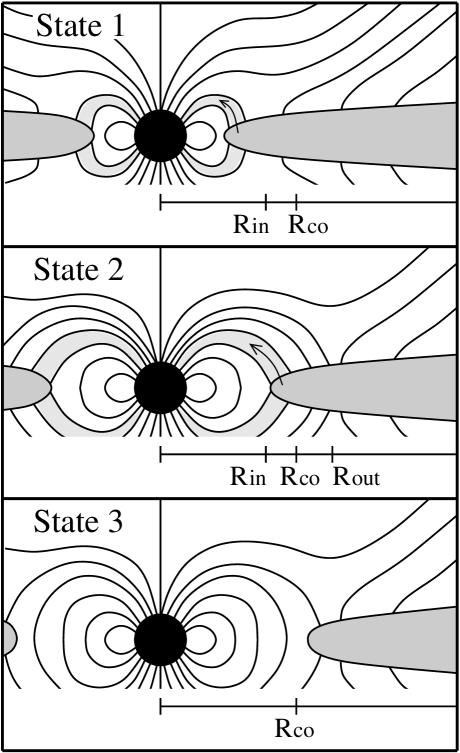
Figure 3: Three possible configurations of the magnetic star-disc interaction. There are two possible accreting states: either the stellar field connects only to the inner edge of the disc (top panel) or it connects to an extend region, reaching beyond $R_{\rm co}$ (middle panel). In either case, the stellar field dominates the accretion flow (arrows) onto the star. Under certain conditions (e.g., low $\dot{M}_{\rm a}$), accretion onto the central star will cease, defining the third, non-accreting state (bottom panel).

The inner edge of the disc is delimited by $R_{\rm t}$ (discussed in §2.3.1), and so there are two possible magnetic configurations of an accreting system, depending on the location of $R_{\rm t}$ relative to $R_{\rm in}$. First, if $R_{\rm t}<R_{\rm in}$, the stellar field will be largely open, and equation 8 is not valid anywhere. The outer radius of the magnetically connected region, $R_{\rm out}^{\prime}$ (which is not then determined by eq. 10) will be near the inner edge of the disc ($R_{\rm out}^{\prime}\sim R_{\rm t}$). We will refer to this situation as ’state 1’ of the system. In state 1, the star receives no spin-down torques from the disc.

In ‘state 2,’ $R_{\rm in}<R_{\rm t}<R_{\rm co}$ and the star is magnetically connected to the disc from $R_{\rm t}$ to $R_{\rm out}$. State 2 represents the typical configuration considered in many models and was discussed at the beginning of this section. Also, systems near their disc-locked state (§3) are always in state 2.

Finally, there exists a third possible, non-accreting state, ’state 3,’ that occurs when the disc is overpowered by the magnetic field (e.g., for fast rotation, large $\mu$, or small $\dot{M}_{\rm a}$) and the disc becomes truncated outside $R_{\rm co}$ (e.g., Illarionov & Sunyaev, 1975). In state 3, there are no positive (spin-up) torques on the star, so it can never be in spin equilibrium (Sunyaev & Shakura, 1977b).

Figure 3 illustrates the basic magnetic configuration of each state. One can think of this Figure, for example, as a sequence (from top to bottom) of decreasing $\dot{M}_{\rm a}$ (or increasing $\mu$). A steadily decreasing $\dot{M}_{\rm a}$ may represent an evolutionary sequence (e.g.) for protostars as one goes from class 0 sources to weak-lined T Tauri stars (class 3). As $\dot{M}_{\rm a}$ decreases from a system in state 1, the disc truncation radius (which is at the inner edge of the disc in the Fig.) moves outward and eventually crosses the location of $R_{\rm in}$ (entering state 2) and then $R_{\rm co}$ (state 3).

The conditions for which a system transitions from an accreting state to state 3 is unknown (see Rappaport et al., 2004 and §4.2.3). In the current work, we do not consider state 3, other than to note that it occurs somewhere below the lower $\dot{M}_{\rm a}$ limit of accreting systems. Instead, we focus most of our attention on state 2 and discuss state 1, where appropriate.

2.3 Torques between the star and disc

A combination of equations 3 and 8 gives the full radial dependence of the differential magnetic torque in the system,

$${d\tau_{\rm m}\over dr}={f^{8/3}\over\beta}{\mu^{2}\over R_{*}^{4}}\left({r\over R_{\rm co}}\right)^{-4}\left[{1-\left({r\over R_{\rm co}}\right)^{3/2}}\right].$$ (12)

where, for convenience, we have used equation 2 to express the radius in units of $R_{\rm co}$. Furthermore, the angular momentum carried by accreting material through each annulus of a Keplerian disc (of width $dr$ and vertically integrated) equals $d\tau_{\rm a}=0.5\dot{M}_{\rm a}(GM_{*}/r)^{-1/2}dr$ (e.g., Clarke et al., 1995). This can be combined with equation 2 to give the differential accretion torque, as a function of $r/R_{\rm co}$,

$${d\tau_{\rm a}\over dr}={1\over 2}\dot{M}_{\rm a}f^{1/3}\left({GM_{*}\over R_{*}}\right)^{1/2}\left({r\over R_{\rm co}}\right)^{-{1/2}}.$$ (13)

The assumption that $\dot{M}_{\rm a}$ is constant at all radii in the disc, requires that the net angular momentum transported away from each annulus in the disc equals $d\tau_{\rm a}$. The disc must therefore be structured in such a way that the differential torques internal to the disc, $d\tau_{\rm i}$, satisfy

$$d\tau_{\rm i}\equiv d\tau_{\rm a}-d\tau_{\rm m}.$$ (14)

These internal torques could result from angular momentum transport via (e.g.) turbulent viscosity (Shakura & Sunyaev, 1973), MRI (Balbus & Hawley, 1991), or disc winds (see review by Königl & Pudritz, 2000). If one assumes a particular angular momentum transport mechanism in the disc, the solution to equation 14 determines the structure of the disc. As an example, for the case of $\alpha$ viscosity, Rappaport et al. (2004) showed that the disc can respond to external magnetic torques by increasing its surface density in order to transport the additional angular momentum outward. A detailed treatment of the disc adjustment is not necessary here, since we are presently concerned with torques on the star, and we simply assume that the disc structures itself such that equation 14 is valid.

Figure 4: Differential torques in the fiducial CTTS system (see discussion above §2.1) for $\beta=1$ and $\gamma_{\rm c}\rightarrow\infty$, where the field is assumed to remain connected over the entire disc. The truncation radius, $R_{\rm t}$, is where $d\tau_{\rm m}=d\tau_{\rm a}$ and $d\tau_{\rm i}=0$, indicated by the vertical dotted line ($R_{\rm t}\approx 0.91R_{\rm co}$). The system is shown in its equilibrium state, where the net torque on the star is zero, requiring a stellar spin period of 6.0 days ($R_{\rm co}\approx 5.5R_{*}$)

Figure 4 shows the differential torques ($d\tau/dr$) as a function of $r/R_{\rm co}$ for the adopted fiducial parameters. The solid, dash-dotted, and dashed lines in Figure 4 represent the differential torques from equations 12, 13, and 14, respectively. The system shown has $\beta=1$ and $\gamma_{\rm c}\rightarrow\infty$, so that the field is connected to the entire surface of the disc, and so that the Figure represents the closed topology of several models in the literature (e.g., AC96).

The differential magnetic torque ($d\tau_{\rm m}$, solid line in Fig. 4) is strongest near the star, where the dipole field is strongest, and it acts to spin up the star (and thus spins down the disc) for $r<R_{\rm co}$ . At $R_{\rm co}$, $d\tau_{\rm m}$ goes to zero, since the field is not twisted ($\gamma=0$) there. Outside $R_{\rm co}$, the magnetic torque becomes stronger again, as the twist increases, though now acting to spin the star down (and the disc up). The dipole field strength falls off faster with distance ($B_{z}\propto r^{-3}$) than the magnetic twist increases ($\gamma\propto r^{3/2}$), so $d\tau_{\rm m}$ has a minimum value at $r/R_{\rm co}\approx 1.37$ and then goes to zero as $r\rightarrow\infty$.

The dashed line in the Figure ($d\tau_{\rm i}$) gives us some information about the disc structure. In this case, the structure will be significantly different than for a case with $d\tau_{\rm m}=0$. For a very large $d\tau_{\rm m}$ outside $R_{\rm co}$, the assumption that the disc can counter act it (via an increase in $d\tau_{\rm i}$) must eventually break down, and the system would then be in state 3 (§2.2).

2.3.1 Truncation radius

Inside the corotation radius, the stellar magnetic torque acts to extract angular momentum from the disc, further enabling accretion (not hindering accretion, as for $r>R_{\rm co}$). The differential magnetic torque increases rapidly as one moves toward the star, and at some point, $d\tau_{\rm m}=d\tau_{\rm a}$. There, the external magnetic torque alone is capable of maintaining $\dot{M}_{\rm a}$. Consequently, $d\tau_{\rm i}$ goes to zero at the same radius and formally becomes negative for smaller $r$ (see Fig. 4). Negative $d\tau_{\rm i}$ is unrealistic, however, since it would require angular momentum transfer inward through the disc, from slower spinning material to faster spinning material, so the Keplerian disc does not exist where where $d\tau_{\rm i}\leq 0$. Thus, the disc truncation radius, $R_{\rm t}$, is where $d\tau_{\rm i}=0$.

At $R_{\rm t}$, the stellar magnetic field will quickly spin down the disc material, forcing it into corotation with the star. Sub-Keplerian rotation leads to a free-fall of disc material onto the surface of the star in a ‘funnel flow’ along magnetic field lines (e.g., K91; Romanova et al., 2002). Whether or not the funnel flow originates exactly from $R_{\rm t}$ or from inside that radius is subject to debate (e.g., Aly & Kuijpers, 1990). However, for the present discussion of angular momentum transport, the most important thing is that $R_{\rm t}$ defines the location where the stellar magnetic field completely dominates over the disc internal stresses, and so all of the angular momentum of disc material at $R_{\rm t}$ will end up on the star.

By setting equation 12 equal to 13, we derive a relationship defining $R_{\rm t}$,

$$\left({R_{\rm t}\over R_{\rm co}}\right)^{-7/2}\left[{1-\left({R_{\rm t}\over R_{\rm co}}\right)^{3/2}}\right]={\beta\over\psi}f^{-{7/3}},$$ (15)

where

$$\psi\equiv 2\mu^{2}\dot{M}_{\rm a}^{-1}(GM_{*})^{-1/2}R_{*}^{-7/2}$$ (16)

is a dimensionless parameter relating the strength of the magnetic field to the strength of accretion. This formula was also derived by Yi (1995), but with different disc parameters in place of our $\beta$. For any given $\beta$, $f$, and $\psi$, there is only one solution to equation 15 such that $R_{\rm t}<R_{\rm co}$. A real system may deviate slightly from our simple picture (e.g., of an unperturbed dipole field), leading to an uncertainty in the exact value of $R_{\rm t}$. However, due to the steep radial dependence of $d\tau_{\rm m}$ relative to $d\tau_{\rm a}$, the location of $R_{\rm t}$ should not be significantly affected. For the system plotted in Figure 4, the solution to equation 15 is $R_{\rm t}/R_{\rm co}\approx 0.915$, represented by the vertical dotted line in the Figure.

For a system in state 1 (with $R_{\rm t}<R_{\rm in}$), equation 15 is not valid because the field will open (see §2.1.3). A substitution of $R_{\rm t}<R_{\rm in}$ in equation 15 indicates that the system will be in state 1 if

$$f<(1-\beta\gamma_{\rm c})(\gamma_{\rm c}\psi)^{-3/7},$$ (17)

and it will be in state 2 for any larger $f$. Note that condition 17 can never be satisfied if $\beta\gamma_{\rm c}\geq 1$ (since $R_{\rm in}$ is then undefined), and so the system would then always exist in state 2. For the more likely case that $\beta\gamma_{\rm c}\ll 1$, state 1 is a possible configuration of any system.

To determine $R_{\rm t}$ in state 1, instead of using equation 12 for the differential magnetic torque, one must consider the maximum possible $d\tau_{\rm m}$ in order that the field remains closed. This is determined by using $\gamma=-\gamma_{\rm c}$ in equation 3. By setting this equal to equation 13, one finds

$$R_{\rm t}=(\gamma_{\rm c}\psi)^{2/7}R_{*}=(2\gamma_{\rm c})^{2/7}(GM_{*})^{-{1/7}}(\dot{M}_{\rm a})^{-{2/7}}\mu^{4/7}.$$ (18)

Note that this equation does not depend on the rotation rate or radius of the star and has the same dependences on other system parameters as in many previous theoretical works (e.g., Davidson & Ostriker, 1973; Ghosh & Lamb, 1979; Shu et al., 1994). Since $R_{\rm t}<R_{\rm in}$ in state 1, the field lines will be open inside $R_{\rm co}$. Thus, in state 1, the stellar field connects only to a small portion of the disc near $R_{\rm t}$, from where a funnel flow originates, and all exterior field lines are open, as shown in the top panel of Figure 3. State 1 is discussed further in section 4.2.

Figure 5: Predicted location of $R_{\rm t}/R_{*}$ as a function of $\log(f)$, for the fiducial CTTS system. The dashed lines represent the prediction from equation 15 for $\beta$ = 0.1, 0.5, 1.0, and 2.0, as indicated, and all have $\gamma_{\rm c}\rightarrow\infty$ so that the magnetic field is assumed to remain closed. The solid line is for $\beta=0.1$, but with $\gamma_{\rm c}=1$, so that the field is partially open. The system with $\gamma_{\rm c}=1$ switches to state 1, for $\log(f)\la-1.5$, and $R_{\rm t}$ is then predicted by equation 18. The dotted line shows the location of $R_{\rm co}$ (eq. 2).

Figure 5 shows the predicted location of $R_{\rm t}$ in units of $R_{*}$ for the adopted fiducial parameters, as a function of the logarithm of the spin rate $f$. For reference, the dotted line shows the location of $R_{\rm co}$ (eq. 2). The dashed lines show $R_{\rm t}$ for systems with $\gamma_{\rm c}\rightarrow\infty$ and $\beta$ = 0.1, 0.5, 1.0, and 2.0, as indicated in the Figure. The solid line shows the $\beta=0.1$ case, but with a more realistic value of $\gamma_{\rm c}=1$. Note that $R_{\rm t}$ is always less than $R_{\rm co}$, and that both decrease as $f$ increases. For stronger field coupling (smaller $\beta$), the field is more strongly twisted, and so $R_{\rm t}$ is closer to $R_{\rm co}$.

All of the dashed lines in Figure 5 represent systems with $\gamma_{\rm c}\rightarrow\infty$, in which the field remains closed for arbitrarily large magnetic twist. Thus, these systems are always in state 2, and the dashed lines are everywhere given by equation 15. On the other hand, the solid line represents a system with $\gamma_{\rm c}=1$, so it is in state 2 only when $f\ga 0.03$ (eq. 17). For smaller $f$, it is in state 1, and $R_{\rm t}$ is then determined by equation 18. Since equation 18 is independent of $f$, state 1 is represented by the constant value of $R_{\rm t}\approx 9.1R_{*}$ in the Figure. Real systems will likely have $\gamma_{\rm c}=1$, in which case the value of $R_{\rm t}\approx 9.1R_{*}$ represents an upper limit for the fiducial CTTS system, regardless $\beta$.

2.3.2 Accretion torque

We assume that accreted disc material is quickly integrated into the structure of the star and the accreted angular momentum is redistributed into the stellar rotation profile. So there is a torque on the steadily accreting star that is given by $\tau_{\rm a}=\dot{M}_{\rm a}[l_{\rm d}(R_{\rm t})-l_{*}]$, where $l_{\rm d}(R_{\rm t})$ is the specific angular momentum of the disc material at $R_{\rm t}$ and $l_{*}$ is that of of the star. Combined with equation 1, and assuming solid body rotation of the star, this becomes

$$\tau_{\rm a}=\dot{M}_{\rm a}(GM_{*}R_{*})^{1/2}\left[{(R_{\rm t}/R_{*})^{1/2}-k^{2}f}\right],$$ (19)

where $k$ is the normalized radius of gyration ($k^{2}\approx 0.2$ for a fully convective star; AC96). This formula is valid for a system in either state 1 or 2.

The term in square brackets in equation 19 is dimensionless and compares the accreting angular momentum (first term) with how much the star already has (second term). Note that the first term will always be greater than or equal to one, while the second term has a maximum value of $k^{2}$ (when $f=1$). Thus, the second term is usually negligible (particularly when $f\ll 1$).

2.3.3 Magnetic torque

When in state 2 (i.e., when $R_{\rm t}>R_{\rm in}$), the stellar field connects to a significant portion of the disc, and one can integrate equation 12 over the connected region, from $R_{\rm t}$ to $R_{\rm out}$, to obtain the total magnetic torque on the star,

$$\tau_{\rm m}={1\over 3\beta}{\mu^{2}\over R_{\rm co}^{3}}\left[{2(R_{\rm co}/R_{\rm out})^{3/2}-(R_{\rm co}/R_{\rm out})^{3}}\right.$$

$$\left.{-2(R_{\rm co}/R_{\rm t})^{3/2}+(R_{\rm co}/R_{\rm t})^{3}}\right].$$ (20)

This torque is independent of the detailed structure of the Keplerian disc. Also, equation 2.3.3 includes the dependence of the magnetic torque on the field topolgy via the variable $R_{\rm out}$. For example, the spin-down torque (found by setting $R_{\rm t}=R_{\rm co}$) exerted by field lines connected out to $R_{\rm out}\approx 2.4R_{\rm co}$ is one half of the spin-down torque for $R_{\rm out}\rightarrow\infty$. Similarly, for $R_{\rm out}\approx 7.2R_{\rm co}$ or $R_{\rm out}\approx 34R_{\rm co}$, the spin-down torque is 90% or 99% (respectively) of the spin-down torque for $R_{\rm out}\rightarrow\infty$. It is evident that, even when $R_{\rm out}$ is large, most of the spin-down torque comes from field lines connected not too far from $R_{\rm co}$. This is simply because the differential magnetic torque (eq. 12) becomes very weak far from the star. Thus the typical assumption of $R_{\rm out}\rightarrow\infty$ is not significantly effected by the fact that real discs have finite radial extents, so long as they reach to several times $R_{\rm co}$.

Above, we have taken $R_{\rm out}$ as arbitrary, but our goal in this paper is to consider the opening of the field from differential rotation, so $R_{\rm out}$ is then given by equation 10, and the preferred formulation of the magnetic torque becomes

$$\tau_{\rm m}={1\over 3\beta}{\mu^{2}\over R_{\rm co}^{3}}\left[{2(1+\beta\gamma_{\rm c})^{-1}-(1+\beta\gamma_{\rm c})^{-2}}\right.$$

$$\left.{-2(R_{\rm co}/R_{\rm t})^{3/2}+(R_{\rm co}/R_{\rm t})^{3}}\right].$$ (21)

This is exactly the solution found by AC96 for the special case of $\beta=1$ and $\gamma_{\rm c}\rightarrow\infty$ (so that $R_{\rm out}\rightarrow\infty$), but our formulation includes the effect of field opening via differential rotation, in which case, the field topology depends on the diffusion parameter $\beta$. The total magnetic torque on the star can be either positive or negative, depending on the size of the connected region inside $R_{\rm co}$, compared to the connected region oustide $R_{\rm co}$. In the next section 2.4, we will show that, for reasonable values of $\beta$ and $\gamma_{\rm c}$, $R_{\rm out}$ is very close to $R_{\rm co}$, and the spin-down torque is significantly effected.

2.4 Effect of opened field

Figure 6: Same as Figure 4, except that the equilibrium spin period is 3.3 days ($R_{\rm co}\approx 3.7R_{*}$), and $\gamma_{\rm c}=1$, so that the magnetic field is not connected for $r>R_{\rm out}\approx 1.6R_{\rm co}$. Also, $R_{\rm t}\approx 0.97R_{\rm co}$.

Figure 6 shows the differential torques in the fiducial CTTS system with $\beta=1$, as in Figure 4. However, unlike Figure 4, here we show the system for $\gamma_{\rm c}=1$, so that the field is open beyond $R_{\rm out}\approx 1.59R_{\rm co}$. The star now rotates significantly faster, with a period of 3.3 days ($f\approx 0.14$), and $R_{\rm t}\approx 0.974R_{\rm co}$. A comparison between Figures 4 and 6 illustrates the effects of varying field topology on the differential torques in the star-disc system.

There are some interesting differences between Figures 4 and 6. Most notably, the differential magnetic torque in Figure 6 abruptly goes to zero at the location of $R_{\rm out}$, due to the assumption that there is no torque on the star from the disc where the field lines are open. It is evident that a more open topology results in a smaller connected region, which leads to a net (integrated) spin-down torque that is smaller than for the completely closed topology. Thus, a more open topology results in a faster equilibrium spin rate, as can be seen by comparing the stellar spin rate of 6.0 days for Figure 4 with 3.3 days for Figure 6.

To quantify the effect of a more open topology on the magnetic torque and to determine the dependence on $\beta$, we first consider only the portion of the magnetic torque that acts to spin down the star by setting $R_{\rm t}=R_{\rm co}$ in equation 2.3.3. For normalization, we use the maximum spin-down torque, $\tau^{\rm max}_{\rm twist}$ (eq. 9). We define the ratio of the true spin-down torque to this maximum torque as $\chi\equiv\tau_{\rm m}(R_{\rm t}=R_{\rm co})/\tau^{\rm max}_{\rm twist}$, which is given by

$$\chi=(\beta\gamma_{\rm c})^{-1}\left[{1+(1+\beta\gamma_{\rm c})^{-2}-2(1+\beta\gamma_{\rm c})^{-1}}\right]$$ (22)

and only depends on the parameter $\beta\gamma_{\rm c}$. It is immediately evident that for $\beta\gamma_{\rm c}=1$, $\chi=1/4$, so the spin-down torque is four times less than used by AC96, when one considers a more realistic magnetic topology.

Figure 7: Logarithm of the ratio of real to maximal spin-down torque (eq. 22), as a function of $\log(\beta\gamma_{\rm c})$. Dotted lines represent $\chi=\beta\gamma_{\rm c}$ and $\chi=(\beta\gamma_{\rm c})^{-1}$.

Figure 7 illustrates the dependence of the torque ratio $\chi$ on $\beta\gamma_{\rm c}$. It decreases as $\beta\gamma_{\rm c}^{-1}$ for $\beta\gg 1$ and increases as $\beta\gamma_{\rm c}$ for $\beta\ll 1$ (as revealed by Taylor expansion of eq. 22). The limiting behavior of $\chi$ is indicated by the two dotted lines in the Figure. This behavior can be understood as a competition between two effects: In the strong magnetic coupling limit ($\beta\ll 1$), the field topology becomes more open for smaller $\beta\gamma_{\rm c}$, reducing the spin-down torque. In the weak coupling limit ($\beta\gg 1$), the topology is largely closed, but the twisting of the field lines is smaller for larger $\beta$, which reduces the differential magnetic torque at all radii ($d\tau_{\rm m}\propto\beta^{-1}$). These two effects conspire to give a maximal value of $\chi$ for the special case of $\beta\gamma_{\rm c}=1$. For the more likely value of $\beta=10^{-2}$, the spin-down torque is two orders of magnitude lower than used by AC96. While it may at first seem surprising that strong magnetic coupling leads to weaker spin-down torques on the star, further reflection reveals that this is necessarily true, since stronger coupling leads to stronger twisting, which further disconnects the star from the disc.

Figure 8: Net torque, $\tau_{\rm a}+\tau_{\rm m}$ (eqs. 19 and 2.3.3), on the star as a function of the logarithm of the fractional spin rate, for the fiducial CTTS system. The four solid lines represent $(\beta,\gamma_{\rm c})=(1,\infty)$, (1, 1), (0.1, 1), and (0.01, 1), as indicated, corresponding to different field topologies, ranging from completely closed to more open. A system will be in spin equilibrium when the net torque equals zero (dotted line).

Finally, equations 19 and 2.3.3 can be used to calculate the net torque on the star. Figure 8 shows this net torque as a function of $\log(f)$ for the fiducial CTTS parameters and for different values of $\beta$ and $\gamma_{\rm c}$. For each case, we calcuate the net torque as follows: First, for a given value of $\beta$ and $\gamma_{\rm c}$, and for each value of $f$, we use equation 17 to determine whether the system is in state 1 or 2. We then find the location of the truncation radius, using equation 15 if the system is in state 2, or equation 18 if in state 1. Finally, we calculate the integrated torques $\tau_{\rm a}$ (eq. 19) and $\tau_{\rm m}$ (eq. 2.3.3, if in state 2; $\tau_{\rm m}=0$, if in state 1). As discussed in section 2.3.1, only cases with $\beta\gamma_{\rm c}<1$ can be in state 1, so only those cases show a transition at $\log f\approx-1.45$ in Figure 8. The Figure also shows the effect of the field topology on the net torque on the star from the disc. It is evident that, when the magnetic field is partially open ($\gamma_{\rm c}=1$), the net torque is larger than for the case where the field is everywhere closed ($\gamma_{\rm c}=\infty$). The spin rate at which the net torque on the star is zero indicates the equilibrium spin state, which is the topic of the next section.

3 The disc-locked state

The general theory presented in section 2 enables one to calculate the net torque ($\tau_{\rm a}+\tau_{\rm m}$) on the star for any accreting system with known $M_{*}$, $R_{*}$, $\mu$, $\dot{M}_{\rm a}$, and $\Omega_{*}$ (one must also adopt a value for $\gamma_{\rm c}$ and $\beta$). The system is stable, in that a positive torque spins the star up, and a faster spin reduces the total torque. Conversely, a negative torque spins down the star, and the torque increases (becoming less negative) for slower spin. Therefore, in a system where the other parameters are relatively constant, the spin rate of the star naturally adjusts to an equilibrium state in which $\tau_{\rm a}+\tau_{\rm m}=0$, known as the ‘disc-locked’ state (e.g., K91; Cameron & Campbell, 1993; Shu et al., 1994; AC96). Since the only torques that spin down the star originate along field lines that connect to the disc outside $R_{\rm co}$, systems in their equilibrium state must be in state 2 ($R_{\rm t}>R_{\rm in}$, see Fig. 3). In this section, we show that both $R_{\rm t}$ and $\Omega_{*}$ in the disc-locked state are significantly affected by the field topology and thus have a strong dependence on the magnetic diffusion parameter $\beta$.

3.1 Truncation radius in the disc-locked state

The disc-locked state is defined by the condition, $\tau_{\rm m}=-\tau_{\rm a}$. Thus, by combining equations 19 and 2.3.3, and using equations 2 and 15 to eliminate $f$, this condition can be rearranged to be

$${{{K(\beta\gamma_{\rm c})-\left({R_{\rm co}/R_{\rm t}}\right)^{3/2}_{\rm eq}}}\over\left({R_{\rm co}/R_{\rm t}}\right)^{{3/2}}_{\rm eq}\left[{1-\left({R_{\rm co}/R_{\rm t}}\right)^{3/2}_{\rm eq}}\right]}=7,$$ (23)

where

$$K(\beta\gamma_{\rm c})\equiv 2(1+\beta\gamma_{\rm c})^{-1}-(1+\beta\gamma_{\rm c})^{-2},$$ (24)

and the subscript ‘eq’ refers to the value in the disc-locked state. In deriving equation 23, we have ignored the term proportional to $k^{2}f$ in equation 19, as justified in the discussion following that equation. The function $K(\beta\gamma_{\rm c})$ characterizes the topology of the field in a sense that, when $\beta\gamma_{\rm c}$ varies between 0 and $\infty$, $K$ varies between 1 (completely open field) and 0 (completely closed). Equation 23 has exactly one solution such that $(R_{\rm t}/R_{\rm co})_{\rm eq}<1$ (which is the only physical solution) for any given $\beta\gamma_{\rm c}>0$.

The location of $R_{\rm t}$ for accreting systems is, in principle, an observable parameter. For example, Kenyon et al. (1996) used a magnetic accretion model to predict infrared excesses in CTTS’s and then to determine the value of $R_{\rm t}/R_{\rm co}$ for a sample of stars in the Taurus-Auriga molecular cloud. The value of $(R_{\rm t}/R_{\rm co})_{\rm eq}$ predicted by equation 23 represents the value for a system that is disc locked.

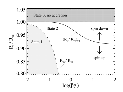
Figure 9: Location of $R_{\rm t}/R_{\rm co}$ in the disc-locked state (solid line; eq. 23), as function of $\log(\beta\gamma_{\rm c})$. The dashed lines represent $R_{\rm in}/R_{\rm co}$ and the location where $R_{\rm t}/R_{\rm co}=1$. Any system with $R_{\rm t}>R_{\rm co}$ is in state 3 (dark grey shaded region), while any system with $R_{\rm t}<R_{\rm in}$ is in state 1 (light grey). Furthermore, if $R_{\rm t}/R_{\rm co}$ is anywhere below (above) the solid line, the net torque from the disc will spin the star up (down).

The solid line in Figure 9 shows $(R_{\rm t}/R_{\rm co})_{\rm eq}$ as a function of $\log(\beta\gamma_{\rm c})$. When a closed field topology is assumed ($\gamma_{\rm c}\rightarrow\infty$), $(R_{\rm t}/R_{\rm co})_{\rm eq}\approx 0.915$. However, for the more reasonable value of $\gamma_{\rm c}=1$, $(R_{\rm t}/R_{\rm co})_{\rm eq}$ increases (approaching unity) as the magnetic coupling becomes stronger (smaller $\beta$). This confirms the conclusion of Wang (1995, and see , ) that any disc-locked system will have $(R_{\rm t}/R_{\rm co})_{\rm eq}\ga 0.9$, and we find that the effect of a more open field topology is to significantly increase this value.

The Figure also indicates the three possible states of the system (discussed further in §4.2), determined by the location of $R_{\rm t}$ relative to $R_{\rm in}$ and $R_{\rm co}$ (dashed lines). A system that is disc-locked is always in state 2. If a system is observed with $R_{\rm t}/R_{\rm co}$ larger than the solid line in the Figure, the star should be spinning down. Conversely, if $R_{\rm t}/R_{\rm co}$ is smaller than the solid line in the Figure, the net torque from accretion and from field lines connecting the star and disc will act to spin the star up. It is interesting that Kenyon et al. (1996) found typical values of $R_{\rm t}/R_{\rm co}$ in the range of 0.6 to 0.8 for the stars in their sample. If true, these stars cannot be in spin equilibrium, unless they feel significant spin-down torques other than those from field lines connecting them to their discs. Furthermore, if $\beta\gamma_{\rm c}<0.3$ is appropriate, the stars in their sample should exist in state 1.

3.2 Stellar spin rate in equilibrium

Now that we can calculate $(R_{\rm t}/R_{\rm co})_{\rm eq}$ via equation 23, we rewrite equation 15 to find the fractional spin rate of the star in equilibrium

$$f_{\rm eq}=C(\beta,\gamma_{\rm c})(2/\psi)^{3/7},$$ (25)

where

$$C(\beta,\gamma_{\rm c})\equiv\left\{{{2\over\beta}\left({R_{\rm co}\over R_{\rm t}}\right)^{2}_{\rm eq}\left[{\left({R_{\rm co}\over R_{\rm t}}\right)^{3/2}_{\rm eq}-1}\right]}\right\}^{-3/7}.$$ (26)

Since $(R_{\rm co}/R_{\rm t})_{\rm eq}$ depends only on $\beta\gamma_{\rm c}$ (via eqs. 23 and 24), the dimensionless function $C(\beta,\gamma_{\rm c})$ depends only on $\beta$ and $\gamma_{\rm c}$. We can also combine equations 1, 16, and 25 to find the equilibrium angular spin rate of the star

$$\Omega_{*}^{\rm eq}=C(\beta,\gamma_{\rm c})\dot{M}_{\rm a}^{3/7}\left({GM_{*}}\right)^{5/7}\mu^{-{6/7}}.$$ (27)

This equation has the same dependence of $\Omega_{*}^{\rm eq}$ on $\dot{M}_{\rm a}$, $M_{*}$, and $\mu$ as equation 3 of K91, and as in the theory of Shu et al. (1994, and , ). The only difference is the value of the factor $C$ used in the various theories. K91 used $C\approx 1.15$, and Ostriker & Shu (1995) found $C\approx 1.13$. However, our formulation of the problem allows us to determine the effect of the field topology on the equilibrium spin rate, via the function $C(\beta,\gamma_{\rm c})$, for arbitrary values of the diffusion parameter $\beta$.

Figure 10: Spin rate factor $C(\beta,\gamma_{\rm c})$ (eq. 26) as a function of $\log(\beta)$. The dotted line is $C(\beta)$ for $\gamma_{\rm c}\rightarrow\infty$ and represents the assumption of a completely closed magnetic topology. The solid line shows the more realistic case with a partially open topology ($\gamma_{\rm c}=1$). The dashed lines represents $C\approx 1.15$ from K91. The Figure is from Matt & Pudritz (2004).

Figure 10 reveals the dependence of $C(\beta,\gamma_{\rm c})$ on $\beta$ for the two values of $\gamma_{\rm c}$ we have considered throughout. For $\gamma_{\rm c}\rightarrow\infty$, $C(\beta)\approx 1.59\beta^{3/7}$, which is represented by the dotted line in the Figure. The solid line shows $C(\beta,\gamma_{\rm c})$ for the more realistic value of $\gamma_{\rm c}=1$ and illustrates the effect of a reduced magnetic connection to the disc. For comparison, the dashed line shows the spin rate factor used by K91, which also roughly represents the typical factors of order unity used in most star-disc interaction models.

The dotted line in Figure 10 represents the assumption that the magnetic field everywhere connects to the disc, regardless of the field twist. In that case, the magnetic torque increases with with decreasing $\beta$, since the field then becomes highly twisted, and so the prediction is that $\Omega_{*}^{\rm eq}\propto\beta^{3/7}$. However, when one considers that dipole field lines will become open when largely twisted, the torque has a maximum value for $\beta=1$ and decreases for any other $\beta$ (see §2.4). Correspondingly, the solid line in Figure 10 has a minimum value for $\beta=1$. This minimum value represents the ‘best case’ for disc locking, and even at this location, $C$ is a factor of 1.8 larger than the value for $\gamma_{\rm c}\rightarrow\infty$ and 2.5 times larger than used by K91. For the more likely value of $\beta=10^{-2}$, the predicted equilibrium spin rate of the star is more than an order of magnitude faster than prediced by any other model. Note that the spin rates of the system plotted in Figures 4 and 6 were chosen to be in equilibrium, and a comparison between the two Figures shows the effect of field topology for the $\beta=1$ ‘best case.’

Figure 11: Equilibrium spin period as a function of observable parameters $\dot{M}_{\rm a}$ (upper left), $B_{*}$ (upper right), $M_{*}$ (lower left), and $R_{*}$ (lower right). In each panel, all parameters are held fixed at the fiducial value except for that which is plotted along the abscissa. The vertical dotted line in each panel shows the fiducial value that is held fixed in the other panels. The solid line in each panel represents the assumption that the magnetic field topology is completely closed ($\gamma_{\rm c}\rightarrow\infty$) and $\beta=1$. All of the broken lines represent a partially open topology ($\gamma_{\rm c}=1$) for $\beta=1$ (dash-dot lines), 0.1 (dashed lines), and the more likely value of 0.01 (dotted lines).

Matt & Pudritz (2004) applied the analysis presented in this section to the CTTS BP Tau, which is one of the few stars for which all of the relevant system parameters are known (or well-constrained). They argued that the existence of slowly rotating, accreting stars, such as BP Tau, cannot be explained by a disc-locking scenario. To further illustrate the effect of field topology on the predictions of disc-locking, and to apply the analysis to all CTTS’s, we have plotted Figure 11. The Figure shows the predicted spin period for a wide range of observable parameters. The spin period is given by $2\pi/\Omega_{*}^{\rm eq}$, and we have used the relationship $\mu=B_{*}R_{*}^{3}$.

The solid lines are for $\gamma_{\rm c}\rightarrow\infty$ and $\beta=1$, and so they represent the ‘standard prediction’ by previous models. The broken lines take into account that some of the field should be open ($\gamma_{\rm c}=1$) for the three different values of $\beta=1$, 0.1, and 0.01. Note that $\beta=0.1$ predicts the same period as for $\beta=10$ (due to the approximate symmetry of the solid line in Fig. 10), and $\beta=0.01$ corresponds with $\beta=100$. It is evident that, even in the ‘best case’ ($\beta=1$) for the disc-locking scenario, the effect of a more open topology is to reduce the equilibrium spin period by a factor of two, compared to the closed field assumption. Given the uncertainties in some of the observed parameters, it may not yet be possible to constrain the predicted period to within a factor of two. In particular, a difference of a factor of two in the predicted spin period could result from an error of a factor of 5.0, 2.2, 2.6, or 1.3 in the observed parameters $\dot{M}_{\rm a}$, $B_{*}$, $M_{*}$, or $R_{*}$, respectively. However, for the more likely value of $\beta=10^{-2}$ (dotted lines in Fig. 11), the predicted spin period is an order of magnitude lower than the ‘standard prediction,’ which cannot be reconciled by observational errors.

3.3 Time to reach equilibrium

It is important to determine how quickly the star will spin up or down to reach the equilibrium state. Rather than fully solving the time-dependent problem, which should also include the spin-up due to the contraction of the protostar (e.g., Yi, 1994), one typically estimates a characteristic spin-down time using the angular momentum of the star, $L_{*}$, divided by the net torque on the star. To be more precise, and for arbitrary spin rates, one should replace $L_{*}$ with the difference between the current $L_{*}$ and the value of $L_{*}$ for the equilibrium spin rate. Assuming solid body rotation of the star, the characteristic time to reach spin equilibrium is then

$$t_{\rm spin}=M_{*}k^{2}R_{*}^{2}\left({{\Omega_{*}^{\rm eq}-\Omega_{*}}\over{\tau_{\rm a}+\tau_{\rm m}}}\right),$$ (28)

which corresponds to a spin-up (down) time for a star currently spinning slower (faster) than $\Omega_{*}^{\rm eq}$. If $t_{\rm spin}$ is long compared to the time-scale for other system parameters to change (e.g., compared to the lifetime of the disc), the star is unlikely to ever be in a spin equilibrium state.

Figure 12: Time to reach equilibrium, $t_{\rm spin}$ (eq. 28), as a function of the spin rate fraction $f$, for the fiducial CTTS system. The four solid lines represent $(\beta,\gamma_{\rm c})=(1,\infty)$, $(1,1)$, $(0.1,1)$, and $(0.01,1)$, as indicated. The vertical dotted lines indicate the equilibrium spin rate, for each case.

Figure 12 shows $t_{\rm spin}$ for the adopted fiducial parameters, as a function of the spin rate fraction $f$ and for different values of $\beta$ and $\gamma_{\rm c}$. It is evident from the Figure that $t_{\rm spin}$ generally decreases for increasing $f$, since faster spin means $R_{\rm co}$ is closer to the star so the magnetic torque will be stronger (whether it spins the star up or down). There is an exception to this when the star spins much slower than $f_{\rm eq}$. For example, for the case with $(\beta,\gamma_{\rm c})$ = (0.01, 1), when $f\la 0.2$, $t_{\rm spin}$ decreases with decreasing $f$. This can be understood, since then $R_{\rm t}/R_{\rm co}$ decreases rapidly with decreasing $f$ (see Fig. 5), leading to much stronger magnetic spin-up torques. Note also that the cases with $(\beta,\gamma_{\rm c})$ = (0.01, 1) and (0.1, 1) are in state 1 for $f\la 0.036$ and 0.033, respectively, in which $\tau_{\rm m}=0$.

For the ‘standard’ prediction with $(\beta,\gamma_{\rm c})$ = (1, $\infty$), $t_{\rm spin}$ is always less than $5\times 10^{4}$ years, which is much shorter than the expected disc lifetime of more than $10^{6}$ years (Muzerolle et al., 2000). However, when one considers the effect of a more open field topology ($\gamma_{\rm c}=1$), the magnetic torques is reduced, and so $t_{\rm spin}$ is longer and increases when $\beta$ decreases. For the likely case with $(\beta,\gamma_{\rm c})$ = (0.01, 1), $t_{\rm spin}\sim 4\times 10^{5}$ years. This is still relatively short compared to the expected disc lifetime. Therefore, we agree with previous authors (e.g., K91; AC96) that systems such as those considered above should exist near their equilibrium spin states throughout most of their accretion lifetimes, but only if $\beta\ga 0.01$. However, the effect of a more open field topology is that the equilibrium spin rate is much faster than previously predicted.

We note in passing that the characteristic time $t_{\rm spin}$ we have calculated here is significantly shorter than recently calculated by Hartmann (2002). Hartmann’s estimate assumes that the upper limit to the spin-down torque on the star is equal to $\dot{M}_{\rm a}(GM_{*}R_{\rm out})^{1/2}$. However, as discussed in section 2.3, this is the torque necessary to provide a steady accretion rate of $\dot{M}_{\rm a}$ through the radius $R_{\rm out}$. In order for the disc to exert a spin-down torque on the star (via the magnetic connection), it must provide a torque in addition to $\dot{M}_{\rm a}(GM_{*}R_{\rm out})^{1/2}$, requiring the disc to have a different structure than in the absence of a stellar field (see Rappaport et al., 2004). It is not yet clear to what extent the disc can be restructured (before accretion will cease), and so Hartmann’s estimate does not represent a true limit.

4 Discussion and conclusions

We extended the standard picture of the interaction of magnetized star with a steady-state accretion disc. Our more comprehensive formulation of this problem allows us to determine the location of the disc truncation radius $R_{\rm t}$ and calculate the torque on the star for a system with arbitrary values of $\dot{M}_{\rm a}$, $\Omega_{*}$, $M_{*}$, $R_{*}$, $B_{*}$, and $\beta$, which parametrizes the coupling of the magnetic field to the disc. We consider only two sources for the torques: (a) torque from the angular momentum deposited by accretion of disc material from $R_{\rm t}$, and (b) torques exerted by field lines connecting the star to the disc over the region from $R_{\rm t}$ to $R_{\rm out}$.

Our model resembles several previous studies (e.g., AC96), except that we have now determined the dependence of the torques on the magnetic coupling to the disc. Specifically, the differential rotation between the star and disc results in a largely open topology (e.g., UKL), so the size of the region of the disc that is magnetically connected to the star is smaller (i.e., $R_{\rm out}$ is smaller). Thus, when one considers this effect, the magnetic spin-down torque on the star is less than if one assumes the field remains everywhere closed. The strongest spin-down torque occurs for intermediate magnetic field coupling ($\beta=1$), in which case the spin-down torque is a factor of four less than for the closed field assumption. For strong magnetic coupling ($\beta\ll 1$), as expected near the inner edge of an accretion disc, $R_{\rm out}$ is very close to $R_{\rm co}$, and the spin-down torque then is proportional to $\beta$. For the likely value of $\beta=0.01$, the spin-down torque is 100 times less than for the closed field assumption! Furthermore, the possibility that field lines may open inside $R_{\rm co}$ characterizes a new mode (state 1) in the system, in which the star feels no spin-down torques from field lines connected to the disc. Three possible system states are summarized in section 4.2.

We also considered the disc-locked state of the system, in which the net torque on the star is zero. A more open field topology leads to an equilibrium state that has a higher stellar spin rate. The time for a given system to reach spin equilibrium is also longer when the field is more open. These results apply to any system in which accretion occurs onto a magnetized central object. In the general case, not all of the system parameters are observationally known. Thus, one often assumes that a particular system is disc-locked, and then ‘tunes’ the unknown system parameter(s) to satisfy equation 27. We found that, equation 27 contains the function $C(\beta,\gamma_{\rm c})$, which is plotted in Figure 10 (solid line), as a function of $\beta$. It is evident, that when the coupling of the field to the disc is strong ($\beta\ll 1$) or weak ($\beta\gg 1$), the ‘tunable’ system parameters will be significantly different than for the usual assumption that $C(\beta,\gamma_{\rm c})$ is a constant near unity. In particular, systems that are thought to be disc-locked will require a larger $\mu$, larger $\Omega_{*}^{\rm eq}$, smaller $M_{*}$, or smaller $\dot{M}_{\rm a}$ than calculated using previous formulations of equation 27. In the next section, we discuss the implications of these results, and recent results from the literature, for disc-locking in CTTS’s.

4.1 Problems with disc locking for CTTS’s

Observational support for disc locking in CTTS’s is still controversial (in particualar, see Stassun et al., 1999; Herbst et al., 2000; Stassun et al., 2001; Herbst et al., 2002), so we have taken another look at the problem from a theoretical standpoint. We find that spin-down torques on a CTTS are significantly reduced for strong coupling of the stellar field to the disc (small $\beta$), resulting in equilibrium spin periods as low as a few days or less, for a wide range of system parameters (see Fig. 11). Small values of $\beta$ are likely for CTTS’s (see §2.1), although $\beta$ is a highly uncertain parameter to calculate from first principles and may even vary from system to system. Also, as discussed in section 2.1.2, there may exist special circumstances that allow the field to remain connected, but whether these circumstances can exist in CTTS systems remains to be shown. Therefore, while our analysis of the problem (in §3) does not completely rule out the possibility for disc locking in all systems (particularly for fast rotators), it significantly reduces the likelyhood that disc-locking can explain the existence of accreting stars spinning at $\sim 10$% (e.g., Bouvier et al., 1993) of break-up speed. There are several other issues in recent literature that, when combined with our analysis, cast additional doubt on the applicability of disc-locking to the slow rotators .

The most notable observational challenge to the disc-locking model is the apparent lack of strong dipole fields on CTTS’s (first suggested by Safier, 1998). It is generally accepted that CTTS’s have field strengths of a few kiloguass. This was predicted by K91, and subsequent observations (Basri et al., 1992; Guenther et al., 1999; Johns-Krull et al., 1999; Johns-Krull & Valenti, 2000; Johns-Krull et al., 2001) have indeed found a mean field on the surface of the central stars of typically 2 kG. Thus far in our analysis, we have adopted a field strength of 2 kG to represent a typical CTTS system and guide our discussion. However, stringent measurements of the mean line of sight field have been carried out for three CTTS’s, BP Tau (Johns-Krull et al., 1999), TW Hya (Johns-Krull & Valenti, 2001), and T Tau (Smirnov et al., 2003, 2004), and all measurements give an upper limit of roughly 200 G for the strength of the dipole component of the stellar magnetic field. The measured mean fields of 2 kG thus represent a field that is disordered or characterized by multipoles of higher order than a dipole (Johns-Krull et al., 1999). Such high order fields, even if very strong on the stellar surface, decrease in strength too quickly with increasing radius to exert significant spin-down torques, especially for slow rotators in which $R_{\rm co}$ is at several stellar radii. Furthermore, a 200 G dipole field cannot exert a significant spin-down torque on a CTTS, even if the field connects to the disc everywhere outside $R_{\rm co}$. This is evident, for example, in the upper right panel of Figure 11, which indicates that the equilibrium spin period for a star with such a field is less than one day. For the cases with $\gamma_{\rm c}=1$ and $\beta\la 0.1$, there is no equilibrium possible, since the magnetic spin-down torques are not strong enough to counteract the angular momentum added by accretion, even for maximal stellar spin ($f=1$). Also, the time to reach equilibrium (for cases in which equilibrium is possible; as discussed in §3.3) increases by an order of magnitude when $B_{*}$ = 200 G, compared to 2 kG.

Second is the issue pointed out by Wang (1995) and discussed in section 3.1 that stars in their disc-locked state must have $R_{\rm t}/R_{\rm co}\ga 0.9$, for a wide range of possible assumptions in the model. Interestingly, Kenyon et al. (1996) concluded that, for their CTTS sample, the typical value of $R_{\rm t}/R_{\rm co}$ was in the range of 0.6 to 0.8, well below the disc-locked value. If true, these stars cannot be disc-locked, since the sum of the accretion torque and the torque carried by field lines connected to the disc will be positive (spinning the stars up; see §2.3.3 and 3.1). Thus, these stars can only be in spin equilibrium if they feel significant spin-down torques other than those from field lines connecting them to their discs. This conclusion does not depend on whether or not the stellar field can open, since the calculation of $R_{\rm t}$ in equilibrium also does not.

Finally, CTTS’s may drive stellar winds (Safier, 1998), and outflows from the disc are known to explain several aspects of observed protostellar outflows (e.g. Königl & Pudritz, 2000). Ionized winds escape from regions with open magnetic field lines, or they can themselves open the field (e.g., as in the solar wind; Parker, 1958), disconnecting the star and disc. Safier (1998) concluded that CTTS’s winds should open all stellar field lines beyond roughly 3 $R_{*}$. Furthermore, a recent measurement of rotation in the jet from the CTTS DG Tau (Bacciotti et al., 2002, and see Testi et al., 2002) suggests that the low velocity component ($\sim 70$ km s^-1) originates in the disc from as close as 0.3 AU from the star (Anderson et al., 2003). This is likely an upper limit (Pesenti et al., 2004), and the more tightly collimated, high velocity component ($\sim 220$ km s^-1; Pyo et al., 2003) must then originate from well within this radius in the disc (Anderson et al., 2003). Theoretical disc-wind models (e.g., Königl & Pudritz, 2000) predict jet speeds of the order of the Keplerian velocity from where the wind is launched, and observed protostellar jets typically travel with speeds of a few hundred km s^-1 (e.g., Reipurth & Bally, 2001). Considering a star with $M_{*}=0.5M_{\odot}$ and $R_{*}=2R_{\odot}$, and assuming $v_{\rm k}=100$ km s^-1 at the launch point, this requires the disc winds to originate from near $GM_{*}/v_{\rm k}^{2}\approx 4.8R_{*}$. These ionized disc winds prevent the star from being magnetically connected to the disc beyond the innermost location of the wind launching point (effectively giving an upper limit to $R_{\rm out}$), and these winds carry angular momentum from the disc, not from the star. As calculated in this paper, a reduced size of the connected region leads to a reduced spin-down torque on the star, regardless of the cause of the field opening. Protostellar outflows thus provide an independent and stringent constraint on disc-locking models.

We conclude that spin-down torques exerted by field lines connecting the star to the disc outside $R_{\rm co}$ are likely to be much weaker than usually assumed. Therefore, the existence of slowly rotating ($f\la 0.1$, or perhaps higher) CTTS’s probably cannot be explained by a disc-locking scenario. Either these stars are all in the process of spinning up, or the stars feel torques other than those related to a magnetic connnection to the accretion disc. Given that the typical spin-up times for these systems are short (see §3.3), the latter possibility appears the most likely.

4.2 Three states of the system

We identified three possible configurations of the system, determined by the location of $R_{\rm t}$, relative to the two key radii $R_{\rm in}$ (eq. 11) and $R_{\rm co}$. There are two accreting configurations, which we call states 1 and 2, and one non-accreting configuration, state 3. Here, we summarize the conditions that determine and characterize each state.

Figure 3 illustrates the basic magnetic configuration of the three states, which may even represent an evolutionary sequence for a system with (e.g.) an evolving $\dot{M}_{\rm a}$ (see §2.2). Figure 9 shows the location of $R_{\rm in}/R_{\rm co}$ (curved, dashed line) for various values of $\beta\gamma_{\rm c}$, and the horizontal dashed line represents the location of $R_{\rm co}$. For a system with a given value of $\beta\gamma_{\rm c}$ and for which $R_{\rm t}$ is determined, the Figure indicates which state the system will be in and whether the star should be spinning up or down.

4.2.1 State 1: $R_{\rm t}<R_{\rm in}$ (or $R_{\rm out}^{\prime}<R_{\rm co}$)

This state is a direct consequence of the opening of field lines via the differential rotation between the star and disc. When $R_{\rm t}$ is sufficiently less than $R_{\rm co}$ (i.e., when $R_{\rm t}<R_{\rm in}$), the magnetic field becomes highly twisted there, opening the field inside $R_{\rm co}$ and resulting in a highly open field topology. Note that state 1, in this context, is only possible for $\beta\gamma_{\rm c}<1$, since otherwise $R_{\rm in}$ is undefined (see Fig. 9 and discussion in §2.1.3).

As illustrated in the top panel of Figure 3 and discussed in section 2.3.1, the stellar field in state 1 connects only to a very small, innermost region of the disc near $R_{\rm t}$, and all exterior field lines are open. The size of the small connected region is likely to be determined by dissipative processes within the disc, but we do not attempt to calculate this here. The location of $R_{\rm t}$ is determined by equation 18 (and see Fig. 5), and accretion onto the star occurs from there.

A star in this state will always feel a net positive torque from the disc, since no field connects outside $R_{\rm co}$. Specifically, the star is spun up by the accretion torque ($\tau_{\rm a}$; eq. 19), and equation 2.3.3 for the magnetic torque is not applicable. In fact, since $R_{\rm t}$ increases with stellar field strength, and since $\tau_{\rm a}\propto R_{\rm t}^{1/2}$, the presence of a stellar field actually increases the spin up torque on the star, relative to non-magnetic accretion. In any case, a system in state 1 cannot be in spin equilibrium, unless it receives torques other than those considered in this paper.

Is state 1 a likely, or even common, configuration for accreting systems? Figure 9 indicates that, when the magnetic coupling to the disc is strong, the range of possible values of $R_{\rm t}$ for which a system can be in state 2 is significantly reduced. For example, if $\beta\gamma_{\rm c}=0.01$, any system with $R_{\rm t}<0.993R_{\rm co}$ should be in state 1. The specific conditions under which any given system will be in state 1 is given by equation 17. For illustrative purposes, we can solve this equation (and using eq. 16) for the mass accretion rate. Assuming $\gamma_{\rm c}=1$, $\beta=0.01$, and $f=0.1$, and using the fiducial CTTS values (see discussion above §2.1), one finds that a system should be in state 1 if

$$\dot{M}_{\rm a}>5.4\times 10^{-7}\left({\gamma_{\rm c}\over 1}\right)\left({1-\beta\gamma_{\rm c}\over 0.99}\right)^{-7/3}\left({M_{*}\over 0.5\;M_{\odot}}\right)^{-1/2}$$

$$\left({B_{*}\over 2\;{\rm kG}}\right)^{2}\left({R_{*}\over 2\;R_{\odot}}\right)^{5/2}\left({f\over 0.1}\right)^{7/3}M_{\odot}\;{\rm yr}^{-1}.$$ (29)

This threshold value of $\dot{M}_{\rm a}$ is an order of magnitude larger than the fiducual value, suggesting that CTTS slow rotators will most commonly exist in state 2.

However, equation 4.2.1 assumes a magnetic field strength of 2 kG, and as discussed in section 4.1, the stars likely have surface dipole field strengths of less than 200 G. This consideration decreases the threshold value of $\dot{M}_{\rm a}$ by at least two orders of magnitude, suggesting that typical CTTS systems may exist in state 1. We can also look at this from the standpoint of stellar spin, using equation 17, which indicates that a system with the adopted fiducial parameters (but with $B_{*}=200$ G) will be in state 1 if it spins more slowly than 26% of break-up speed. (As discussed in section 2.3.1, this also corresponds an upper limit of $R_{\rm t}\la 2.4R_{*}$.) Thus, if the dipole fields are indeed weak, it is more likely that slow rotators, and even some fast rotators, will be in state 1. Furthermore, the conclusion of Kenyon et al. (1996), that $R_{\rm t}/R_{\rm co}$ typically ranges from 0.6 to 0.8, suggests that CTTS’s will be in state 1, as long as $\beta\gamma_{\rm c}<0.3$ (see §3.1).

We have thus far considered the opening of field lines via the differential rotation, so the existence of state 1 requires that $\beta\gamma_{\rm c}$ is significantly less than unity. Given the large uncertainty in the value of $\beta$ in real systems, it is still not clear whether or not state 1 should be common. From the standpoint of torques on the star, the most important feature of state 1 is that the stellar field never connects to the disc outside $R_{\rm co}$. Thus, for the following discussion, we will generalize the definition of state 1 to include any magnetic configuration in which the star does not connect outside $R_{\rm co}$.

State 1 is characterized by a large amount of open stellar field, so it is natural to consider the effects of a stellar wind in the magnetically open region. As discussed in section 4.1, a wind can even be responsible for opening the field (which does not depend on our parameters $\beta$ and $\gamma_{\rm c}$). Thus, if a wind (or any other process) keeps the stellar field open beyond some radius $R_{\rm out}^{\prime}$, and if $R_{\rm out}^{\prime}<R_{\rm co}$, the system will be in state 1. For example, Safier (1998) concluded that stellar winds from CTTS’s could result in $R_{\rm out}^{\prime}\la 3R_{*}$. If true, this means that any system rotating more slowly than 19% of break-up speed will have $R_{\rm out}^{\prime}<R_{\rm co}$ (eq. 1) and be in state 1.

There is empirical evidence for systems in state 1 from some numerical simulations of the star-disc interaction, which usually represent systems with $\beta\ll 1$. In the simulations of Goodson & Winglee (1999) and von Rekowski & Brandenburg (2004), as an example, after the initial state, the stellar field never connects to the disc outside $R_{\rm co}$, even immediately following reconnection events. These authors report that the only significant spin-down torques on the star come from the open field regions (though a stellar wind was not properly included), rather than along field lines connecting the stars to their discs (but also see Romanova et al., 2002).

It seems that state 1 is a likely configuration for accreting stars, particularly among slow rotators. Since, in this state, the net torque from the interaction with the accretion disc only acts to spin up the star, stars with long-lived accretion phases must somehow rid themselves of this excess angular momentum. Stellar winds can exert spin-down torques on the star, and if these torques are significant (e.g., Tout & Pringle, 1992), the equilibrium spin rate may be simply determined by a balance between this torque and $\tau_{\rm a}$. In this situation, state 1 could actually represent the expected configuration for accreting systems in spin equilibrium.

4.2.2 State 2: $R_{\rm in}<R_{\rm t}<R_{\rm co}$

In this state, the stellar field connects to a finite region of the disc between $R_{\rm t}$ and $R_{\rm out}$, as illustrated in the middle panel of Figure 3. This represents the typical configuration in many star-disc interaction models, except that the determination of $R_{\rm out}$ varies between models. The location of $R_{\rm t}$ is determined by equation 15 (and see Fig. 5), and accretion onto the star occurs from there.

The star is spun up by the accretion torque (eq. 19) and magnetic torques (eq. 2.3.3) from field lines connected to the region of the disc between $R_{\rm t}$ and $R_{\rm co}$ and spun down by magnetic torques from field lines connected between $R_{\rm co}$ and $R_{\rm out}$. Therefore, a system can exist in an equilibrium, disc-locked state, in state 2, in which the net torque on the star is zero, and the spin rate of the star then correlates with accretion parameters (see §3).

When one considers that the differential rotation determines $R_{\rm out}$ (via eq. 10), both $\Omega_{*}^{\rm eq}$ and $(R_{\rm t}/R_{\rm co})_{\rm eq}$ are larger for smaller $\beta$. Also, as shown in Figure 9, the range of (non-equilibrium) values of $R_{\rm t}$ that exist in state 2 becomes narrower as $\beta$ decreases. For the strong coupling case of $\beta\gamma_{\rm c}=0.01$, a system can only be in state 2 if $0.993<R_{\rm t}/R_{\rm co}<1.0$. So for strong coupling, it is unlikely that a given system will exist in state 2, unless it is very near its disc-locked state, which then requires a fast stellar spin.

Another intriguing effect of a largely open field topology is that, in order for a system to be disc-locked, the differential magnetic torque in the disc $d\tau_{\rm m}$ must be stronger (compared to the completely closed assumption) in order to make up for the decreased size of the connected region (compare Figs. 4 and 6). When the connected region is very small (i.e., for small $\beta$), $d\tau_{\rm m}$ is very large, which ought to have a significant effect on the disc structure there. There may be a physical limit, beyond which the disc cannot respond, and accretion will cease (see discussion of state 3, below). This could possibly lead to a time-dependent process (e.g., Spruit & Taam, 1993), perhaps analogous to the simulations of (e.g.) Goodson et al. (1999, though their stellar field does not connect outside $R_{\rm co}$), and in which there may still be a time-averaged net torque of zero.

4.2.3 State 3: $R_{\rm t}>R_{\rm co}$

Since no accretion onto the star occurs, state 3 may characterize the non-accreting, weak-line T Tauri phase of pre-main sequence stellar evolution. Also, since the disc does not extend inside $R_{\rm co}$, the star feels no spin-up torques, only spin-down torques, and so it cannot exist in spin equilibrium (Sunyaev & Shakura, 1977b). A possible magnetic field configuration of this state is illustrated in the bottom panel of Figure 3.

It is not yet clear under which conditions a system will be in this state, though the relative values of differential torques (or stresses) in the disc are certainly important. Some authors (e.g., Wang, 1995; Clarke et al., 1995) have speculated that state 3 occurs when $|d\tau_{\rm m}/d\tau_{\rm a}|$ becomes greater than one (Cameron & Campbell, 1993 suggested a value of 2) anywhere outside $R_{\rm co}$. In this work, we have assumed that the disc will be structured such that equation 14 is satisfied (see §2.3 and Rappaport et al., 2004). However, this assumption must eventually break down for large enough $f$, large enough $\mu$, or small enough $\dot{M}_{\rm a}$.

The general question of what conditions govern a system in state 3, to our knowledge, remains an unanswered astrophysical problem. It is not clear what will determine the location of $R_{\rm t}$ in state 3 (since neither of equations 15 and 18 is then valid). In addition to magnetic torques, outflows and/or radiation from the star may be important (Johnstone, 1995). Understanding this state is probably relevant to understanding the transition from classical to weak-line T Tauri phases, and it may even have further implications for gas giant planet formation/migration (Lin et al., 1996; Trilling et al., 2002) and for the ultimate dissipation of the gas disc.

4.3 Conclusions

We have considered that the opening of magnetic field lines expected from differential rotation in the star-disc interaction results in a largely open field topology. This significantly alters the torque that a star receives from its accretion disc, compared to previous models that assume a closed field. Our main conclusions from this work are the following:

1. This more open field topology resuts in a weaker spin-down torque felt by the star from the disc (§2.4). The strongest possible torque occurs for intermediate magnetic coupling to the disc. Stronger coupling, as expected near the inner edge of the disc, results in a spin-down torque that is more than an order of magnitude below the torque found for the closed field assumption.

2. In the disc-locked, spin equilibrium state, this results in a stellar spin rate that is much faster than predicted by previous models (§3.2).

3. We have identified and discussed three possible magnetic field configurations in magnetic star-disc systems (§4.2). The three configurations could represent, for example, an evolutionary sequence for a system with a gradually decreasing mass accretion rate (or, e.g., a gradually increasing stellar spin rate). Our conclusions about each state, in the context of T Tauri stars, are the following:

   1. Assuming strong magnetic coupling to the disc, slowly rotating CTTS’s should be in state 1 if $\dot{M}_{\rm a}\ga 5\times 10^{-9}M_{\odot}$ yr^-1 (eq. 4.2.1 for $B_{*}=200$ G). Since typical accretion rates are higher than this, state 1 may represent a common configuration in these systems. In this state, the star feels no spin-down torques from the disc. However, if spin-down torques from (e.g.) a stellar wind are significant, stars may be in spin equilibrium in state 1, though they should not then be considered ‘disc locked.’

   2. State 2 is the typical configuration assumed in star-disc interaction models. For strong magnetic coupling in the disc, or if stellar or disc winds are important, we find that a system can only be in state 2 under special circumstances. In particular, the accretion rate must be lower than for state 1.

   3. State 3 likely represents the non-accreting, weak-line T Tauri phase. Given that the accretion disc can restructure itself in response to (e.g.) external magnetic torques, it it not yet clear when a system will transition into this state. This important evolutionary phase requires more theoretical study.

4. These considerations, and additional issues from the literature, suggest that slowly rotating CTTS’s probably cannot be explained by a disc-locking scenario (§4.1).

5. If slowly rotating CTTS’s are in spin equilibrium, then another spin down torque must be active in the system. We suggest that this might arise from magnetized stellar winds.

References

- Agapitou & Papaloizou (2000) Agapitou V., Papaloizou J. C. B., 2000, MNRAS, 317, 273
- Aly (1985) Aly J. J., 1985, A&A, 143, 19
- Aly & Kuijpers (1990) Aly J. J., Kuijpers J., 1990, A&A, 227, 473
- Anderson et al. (2003) Anderson J. M., Li Z., Krasnopolsky R., Blandford R. D., 2003, ApJ, 590, L107
- Armitage & Clarke (1996) Armitage P. J., Clarke C. J., 1996, MNRAS, 280, 458 (AC96)
- Bacciotti et al. (2002) Bacciotti F., Ray T. P., Mundt R., Eislöffel J., Solf J., 2002, ApJ, 576, 222
- Balbus & Hawley (1991) Balbus S. A., Hawley J. F., 1991, ApJ, 376, 214
- Bardou & Heyvaerts (1996) Bardou A., Heyvaerts J., 1996, A&A, 307, 1009
- Barnes et al. (2001) Barnes S., Sofia S., Pinsonneault M., 2001, ApJ, 548, 1071
- Basri et al. (1992) Basri G., Marcy G. W., Valenti J. A., 1992, ApJ, 390, 622
- Blandford & Payne (1982) Blandford R. D., Payne D. G., 1982, MNRAS, 199, 883
- Bouvier et al. (1993) Bouvier J., Cabrit S., Fernandez M., Martin E. L., Matthews J. M., 1993, A&A, 272, 176
- Bouvier et al. (1997) Bouvier J., Forestini M., Allain S., 1997, A&A, 326, 1023
- Cameron & Campbell (1993) Cameron A. C., Campbell C. G., 1993, A&A, 274, 309
- Clarke et al. (1995) Clarke C. J., Armitage P. J., Smith K. W., Pringle J. E., 1995, MNRAS, 273, 639
- Davidson & Ostriker (1973) Davidson K., Ostriker J. P., 1973, ApJ, 179, 585
- De Marco et al. (2004) De Marco O., Lanz T., Ouellette J. A., Zurek D., Shara M. M., 2004, ApJ, 606, L151
- Ghosh & Lamb (1978) Ghosh P., Lamb F. K., 1978, ApJ, 223, L83
- Ghosh & Lamb (1979) Ghosh P., Lamb F. K., 1979, ApJ, 234, 296
- Goodson et al. (1999) Goodson A. P., Böhm K., Winglee R. M., 1999, ApJ, 524, 142
- Goodson & Winglee (1999) Goodson A. P., Winglee R. M., 1999, ApJ, 524, 159
- Goodson et al. (1997) Goodson A. P., Winglee R. M., Böhm K. H., 1997, ApJ, 489, 199
- Guenther et al. (1999) Guenther E. W., Lehmann H., Emerson J. P., Staude J., 1999, A&A, 341, 768
- Hartmann (2002) Hartmann L., 2002, ApJ, 566, L29
- Hayashi et al. (1996) Hayashi M. R., Shibata K., Matsumoto R., 1996, ApJ, 468, L37
- Herbst et al. (2002) Herbst W., Bailer-Jones C. A. L., Mundt R., Meisenheimer K., Wackermann R., 2002, A&A, 396, 513
- Herbst et al. (2000) Herbst W., Rhode K. L., Hillenbrand L. A., Curran G., 2000, AJ, 119, 261
- Illarionov & Sunyaev (1975) Illarionov A. F., Sunyaev R. A., 1975, A&A, 39, 185
- Johns-Krull & Gafford (2002) Johns-Krull C. M., Gafford A. D., 2002, ApJ, 573, 685
- Johns-Krull & Valenti (2000) Johns-Krull C. M., Valenti J. A., 2000, in ASP Conf. Ser. 198: Stellar Clusters and Associations: Convection, Rotation, and Dynamos Measurements of stellar magnetic fields. p. 371
- Johns-Krull & Valenti (2001) Johns-Krull C. M., Valenti J. A., 2001, in ASP Conf. Ser. 244: Young Stars Near Earth: Progress and Prospects The Magnetic Field of TW Hydrae. p. 147
- Johns-Krull et al. (1999) Johns-Krull C. M., Valenti J. A., Hatzes A. P., Kanaan A., 1999, ApJ, 510, L41
- Johns-Krull et al. (1999) Johns-Krull C. M., Valenti J. A., Koresko C., 1999, ApJ, 516, 900
- Johns-Krull et al. (2001) Johns-Krull C. M., Valenti J. A., Saar S. H., Hatzes A. P., 2001, in ASP Conf. Ser. 223: 11th Cambridge Workshop on Cool Stars, Stellar Systems and the Sun New Measurements of Magnetic Fields on T Tauri Stars (CD-ROM Directory: contribs/krull). p. 521
- Johnstone (1995) Johnstone D. I., 1995, Ph.D. Thesis
- Joss & Rappaport (1984) Joss P. C., Rappaport S. A., 1984, ARA&A, 22, 537
- Kato et al. (2004) Kato Y., Hayashi M. R., Matsumoto R., 2004, ApJ, 600, 338
- Kato et al. (2001) Kato Y., Hayashi M. R., Miyaji S., Matsumoto R., 2001, Advances in Space Research, 28, 505
- Kenyon et al. (1996) Kenyon S. J., Yi I., Hartmann L., 1996, ApJ, 462, 439
- Königl (1991) Königl A., 1991, ApJ, 370, L39 (K91)
- Königl & Pudritz (2000) Königl A., Pudritz R. E., 2000, in Mannings V., Boss A. P., Russell S. S., eds, Protostars and Planets IV Disk Winds and the Accretion-Outflow Connection. Tucson: Univ. of Arizona Press, p. 759
- Küker et al. (2003) Küker M., Henning T., Rüdiger G., 2003, ApJ, 589, 397
- Leonard & Livio (1995) Leonard P. J. T., Livio M., 1995, ApJ, 447, L121
- Lin et al. (1996) Lin D. N. C., Bodenheimer P., Richardson D. C., 1996, Nature, 380, 606
- Livio & Pringle (1992) Livio M., Pringle J. E., 1992, MNRAS, 259, 23P
- Lovelace et al. (1995) Lovelace R. V. E., Romanova M. M., Bisnovatyi-Kogan G. S., 1995, MNRAS, 275, 244
- Lynden-Bell & Boily (1994) Lynden-Bell D., Boily C., 1994, MNRAS, 267, 146
- Makishima et al. (1999) Makishima K., Mihara T., Nagase F., Tanaka Y., 1999, ApJ, 525, 978
- Matt et al. (2002) Matt S., Goodson A. P., Winglee R. M., Böhm K., 2002, ApJ, 574, 232
- Matt & Pudritz (2004) Matt S., Pudritz R. E., 2004, ApJ, 607, Letters, in press
- Miller & Stone (1997) Miller K. A., Stone J. M., 1997, ApJ, 489, 890
- Muzerolle et al. (2000) Muzerolle J., Calvet N., Briceño C., Hartmann L., Hillenbrand L., 2000, ApJ, 535, L47
- Muzerolle et al. (2001) Muzerolle J., Calvet N., Hartmann L., 2001, ApJ, 550, 944
- Newman et al. (1992) Newman W. I., Newman A. L., Lovelace R. V. E., 1992, ApJ, 392, 622
- Ostriker & Shu (1995) Ostriker E. C., Shu F. H., 1995, ApJ, 447, 813
- Paczynski (1991) Paczynski B., 1991, ApJ, 370, 597
- Parker (1958) Parker E. N., 1958, ApJ, 128, 664
- Patterson (1994) Patterson J., 1994, PASP, 106, 209
- Pesenti et al. (2004) Pesenti N., Dougados C., Cabrit S., Ferreira J., Casse F., Garcia P., O’Brien D., 2004, A&A, 416, L9
- Piirola et al. (1993) Piirola V., Hakala P., Coyne G. V., 1993, ApJ, 410, L107
- Popham & Narayan (1991) Popham R., Narayan R., 1991, ApJ, 370, 604
- Pyo et al. (2003) Pyo T., Kobayashi N., Hayashi M., Terada H., Goto M., Takami H., Takato N., Gaessler W., Usuda T., Yamashita T., Tokunaga A. T., Hayano Y., Kamata Y., Iye M., Minowa Y., 2003, ApJ, 590, 340
- Rappaport et al. (2004) Rappaport S. A., Fregeau J. M., Spruit H., 2004, ApJ, 606, 436
- Rebull et al. (2004) Rebull L. M., Wolff S. C., Strom S. E., 2004, AJ, 127, 1029
- Reipurth & Bally (2001) Reipurth B., Bally J., 2001, ARA&A, 39, 403
- Romanova et al. (2002) Romanova M. M., Ustyugova G. V., Koldoba A. V., Lovelace R. V. E., 2002, ApJ, 578, 420
- Safier (1998) Safier P. N., 1998, ApJ, 494, 336
- Sano et al. (2004) Sano T., Inutsuka S., Turner N. J., Stone J. M., 2004, ApJ, 605, 321
- Shakura & Sunyaev (1973) Shakura N. I., Sunyaev R. A., 1973, A&A, 24, 337
- Shu et al. (1994) Shu F., Najita J., Ostriker E., Wilkin F., Ruden S., Lizano S., 1994, ApJ, 429, 781
- Sills et al. (2001) Sills A., Faber J. A., Lombardi J. C., Rasio F. A., Warren A. R., 2001, ApJ, 548, 323
- Sills et al. (2000) Sills A., Pinsonneault M. H., Terndrup D. M., 2000, ApJ, 534, 335
- Smirnov et al. (2003) Smirnov D. A., Fabrika S. N., Lamzin S. A., Valyavin G. G., 2003, A&A, 401, 1057
- Smirnov et al. (2004) Smirnov D. A., Lamzin S. A., Fabrika S. N., Chuntonov G. A., 2004, Astronomy Letters, in press
- Spruit & Taam (1993) Spruit H. C., Taam R. E., 1993, ApJ, 402, 593
- Stassun et al. (1999) Stassun K. G., Mathieu R. D., Mazeh T., Vrba F. J., 1999, AJ, 117, 2941
- Stassun et al. (2001) Stassun K. G., Mathieu R. D., Vrba F. J., Mazeh T., Henden A., 2001, AJ, 121, 1003
- Sunyaev & Shakura (1977a) Sunyaev R. A., Shakura N. I., 1977a, Pis ma Astronomicheskii Zhurnal, 3, 262
- Sunyaev & Shakura (1977b) Sunyaev R. A., Shakura N. I., 1977b, Pis ma Astronomicheskii Zhurnal, 3, 216
- Testi et al. (2002) Testi L., Bacciotti F., Sargent A. I., Ray T. P., Eislöffel J., 2002, A&A, 394, L31
- Tinker et al. (2002) Tinker J., Pinsonneault M., Terndrup D., 2002, ApJ, 564, 877
- Tout & Pringle (1992) Tout C. A., Pringle J. E., 1992, MNRAS, 256, 269
- Trilling et al. (2002) Trilling D. E., Lunine J. I., Benz W., 2002, A&A, 394, 241
- Uzdensky (2004) Uzdensky D. A., 2004, in Gomez de Castro A. I., Heyer M., Vazquez-Semadeni E., Rebolo R., Tagger M., Pudritz R. E., eds, Magnetic Fields and Star Formation: Theory v. Observations Magnetic Interaction Between Stars and Accretion Disks. Astrophysics and Space Science, Vols 1-4, pp (astro–ph/0310104)
- Uzdensky et al. (2002a) Uzdensky D. A., Königl A., Litwin C., 2002a, ApJ, 565, 1191 (UKL)
- Uzdensky et al. (2002b) Uzdensky D. A., Königl A., Litwin C., 2002b, ApJ, 565, 1205
- von Rekowski & Brandenburg (2004) von Rekowski B., Brandenburg A., 2004, A&A, in press
- Wang (1995) Wang Y.-M., 1995, ApJ, 449, L153
- Yi (1994) Yi I., 1994, ApJ, 428, 760
- Yi (1995) Yi I., 1995, ApJ, 442, 768