QUASARS AND THE BIG BLUE BUMP

Abstract

We investigate the ultraviolet-to-optical spectral energy distributions (SEDs) of 17 active galactic nuclei (AGNs) using quasi-simultaneous spectrophotometry spanning 900–9000Å (rest frame). We employ data from the Far Ultraviolet Spectroscopic Explorer (FUSE), the Hubble Space Telescope (HST), and the 2.1-meter telescope at Kitt Peak National Observatory (KPNO). Taking advantage of the short-wavelength coverage, we are able to study the so-called “big blue bump,” the region where the energy output peaks, in detail. Most objects exhibit a spectral break around 1100Å. Although this result is formally associated with large uncertainty for some objects, there is strong evidence in the data that the far-ultraviolet spectral region is below the extrapolation of the near-ultraviolet-optical slope, indicating a spectral break around 1100Å. We compare the behavior of our sample to those of non-LTE thin-disk models covering a range in black-hole mass, Eddington ratio, disk inclination, and other parameters. The distribution of ultraviolet-optical spectral indices redward of the break, and far-ultraviolet indices shortward of the break, are in rough agreement with the models. However, we do not see a correlation between the far-ultraviolet spectral index and the black hole mass, as seen in some accretion disk models. We argue that the observed spectral break is intrinsic to AGNs, although intrinsic reddening as well as Comptonization can strongly affect the far-ultraviolet spectral index. We make our data available online in digital format.

1 INTRODUCTION

The spectral energy distribution (SED) of AGNs contains a significant feature in the ultraviolet (UV) to optical region, known as “the big blue bump.” This feature is thought to be thermal emission from an optically thick accretion disk feeding a massive black hole (e.g., Shields, 1978; Malkan & Sargent, 1982), and it has been argued that its energy peak lies in the unobserved extreme ultraviolet (EUV, $\sim$100–912Å) region (e.g., Mathews & Ferland, 1987). To determine the shape and the peak of the big blue bump is of particular importance, since this provides critical information on the structure and condition of the inner-most region in AGNs as well as on the ionizing flux that powers the emission lines.

Zheng et al. (1997) constructed composite AGN spectra from HST spectra, and found that the UV-optical power-law continuum breaks at around 1000Å. This was later confirmed in a similar HST composite using a larger sample (Telfer et al., 2002). Laor et al. (1997), also using composite spectra, found that the soft X-ray continuum matches up with the extrapolation of the HST composite, consistent with the idea that the UV bump actually peaks in far-ultraviolet (FUV, 912–2000Å), rather than the EUV. However, such a spectral break is not seen in the recent FUSE composite spectra for low-redshift AGNs (Scott et al., 2004), although some individual sources do show a spectral break. Scott et al. (2004) noted that this FUSE sample has a median luminosity one order of magnitude lower than that of the HST sample (Zheng et al., 1997), and it is possible the break wavelength is luminosity dependent. It is important to realize that composite spectra represent a complex average of many individual spectra. Examination of the individual spectra in a composite may lead to greater insights, and they can be used to understand the overall characteristics of a composite in a more physical way. For instance, the spectrum of 3C273 shows a break near the Lyman limit (Kriss et al., 1999), and reasonable fits to the spectrum with accretion disk models have been reported (Kriss et al., 1999; Blaes et al., 2001).

It is well accepted that AGNs are powered by accretion onto massive black holes. Many accretion disk models have been built to predict the AGN continuum and compare with observed spectra (e.g., Sun & Malkan, 1989; Laor & Netzer, 1989; Laor, 1990; Czerny & Zbyszewska, 1991; Hubeny et al., 2000, 2001). Since the AGN local environment is not well known, and the models are still relatively very simple, it is not possible for the models to predict the detailed features in the observed spectra. However, large-scale features in the AGN SEDs can be reproduced by disk models. Simple models produce a large continuum discontinuity at the Lyman limit, but it is not often seen in real objects (e.g., Koratkar, Kinney, & Bohlin, 1992). Such a feature could be smeared out by relativistic smearing and Comptonization (e.g, Hsu & Blaes, 1998; Kriss et al., 1999; Blaes et al., 2001; Hubeny et al., 2001). This results in a bump or a spectral break, instead of an edge, in the vicinity of Lyman limit, which resembles the spectral breaks seen in some observed AGN spectra. Hubeny et al. (2000) constructed geometrically thin accretion disk models with non-LTE atmospheres, including a full treatment of general relativistic effects in the disk structure. We choose this specific model and compare the spectral properties in the FUV-optical region for a sample of 17 low-redshift AGNs with the model expectations.

We characterize the spectral continuum with broken power-laws. Unless noted, the power-law indices we use through this paper are all $\alpha_{\lambda}$ ($f_{\lambda}\propto\lambda^{\alpha_{\lambda}}$) except that the soft X-ray spectral index $\alpha_{\rm x}$ is $\alpha_{\nu}$ ($f_{\nu}\propto\nu^{\alpha_{\nu}}$). It is easy to convert between $\alpha_{\lambda}$ and $\alpha_{\nu}$ ($\alpha_{\lambda}+\alpha_{\nu}=-2$). For cosmology, we choose $\Lambda=0$, $H_{0}=75\,{\rm km~{}s}^{-1}\mbox{Mpc}^{-1}$, and $q_{0}=0.5$. Since the objects in this sample are at low redshifts, the results in the paper are not affected by the choice of cosmology.

2 SAMPLE AND DATA

The FUSE AGN program (Kriss, 2000) has surveyed more than 100 of the UV-brightest AGNs, of which about 20 were also observed in an HST spectral snapshot survey during 1999–2000. The FUSE observations were scheduled as close in time as possible with the HST snapshot observations. Ground-based optical spectra were also obtained during the same period at KPNO. We excluded a few objects because of the lack of an optical spectrum (NGC 3783, low declination), strong host galaxy contamination (NGC 3516), or strong variability (NGC 5548, also no simultaneous HST spectrum). As a result, we have compiled a sample of 17 AGNs, with quasi-simultaneous spectrophotometry covering rest wavelength from 900–9000Å. This is a heterogeneous sample with low redshift ($z<0.5$).

Table 1: Sample and Observation Log

				Observation Date					Dataset ID		CalFUSE
Object	Other Name	$z$	E(B-V)	FUSE	HST	Opt. Blue	Opt. Red		FUSE ID	HST ID	Version
3C273	PG1226+023	0.1576	0.021	2000-04-23	2000-03-16	2000-02-25	2000-02-26		P1013501	O5G045JZQ , O5G045K0Q	v2.0.5
3C351	PG1704+608	0.3730	0.023	1999-10-17	1992-02-15	1999-10-09	1990-09-20		Q1060101	Y0VM0103T , Y0RV0G04T	v2.2.2
4C+34.47	B2 1721+34	0.2055	0.037	2000-06-09	2000-06-25	1999-10-09	2000-02-27		P1073501	O5G077Y2Q , O5G077Y3Q	v2.2.2
IRAS F07546+3928	MS 0754.6+3928	0.0953	0.066	2002-02-11	2000-01-29	1999-10-09	1999-10-08		S6011801	O5G018LPQ , O5G018LQQ	v2.1.7
MRK290	PG1534+580	0.0303	0.015	2000-03-16	2000-06-02	2000-02-25	2000-02-27		P1072901	O5G070TLQ , O5G070TMQ	v1.8.7
MRK304	PG2214+139	0.0657	0.073	2000-07-16	2000-06-19	1999-10-07	1999-10-08		P1073901	O5G082ANQ , O5G082AOQ	v2.0.5
MRK506		0.0428	0.031	2000-06-08	2000-06-24	1999-10-09	2000-02-27		P1073401	O5G076UEQ , O5G076UFQ	v2.0.5
MRK509		0.0345	0.057	1999-11-06	1992-06-21	1999-12-11	1999-12-11		X0170102	Y0YA0302T , Y0YA0305T	v2.1.7
NGC3516		0.0883	0.042	2000-04-17	2000-04-20				P1110404	O5G032T7Q , O5G032T8Q	v2.1.7
NGC3783		0.0097	0.119	2000-02-02	2000-05-17				P1013301	O5G039LBQ , O5G039LCQ	v1.8.7
PG0052+251		0.1544	0.047	1999-10-03	1999-10-01	1999-10-07	1999-10-08		P1070101	O5G003NAQ , O5G003NBQ	v2.0.5
PG0947+396		0.2057	0.019	2001-01-06	2000-06-15	1999-10-09	2000-02-27		A0600101	O5G023NPQ , O5G023NQQ	v2.2.2
PG0953+414		0.2338	0.013	1999-12-30	2000-02-05	1999-10-09	2000-02-26		P1012202	O5G024NBQ , O5G024NCQ	v2.2.2
PG1100+772	3C249.1	0.3114	0.034	2000-01-20	2000-01-31	1993-05	1993-05		P1071601	O5G030D4Q , O5G030D5Q	v2.2.2
PG1259+593		0.4769	0.008	2000-02-25	2000-02-09	2000-02-25	2000-02-26		P1080101	O5G047IJQ , O5G047IKQ	v2.2.2
PG1322+659		0.1684	0.019	2000-05-08	2000-06-18	2000-02-25	2000-02-26		A0600808	O5G052WXQ , O5G052WYQ	v2.2.2
PG1351+640		0.0882	0.020	2000-01-18	1999-10-28	2000-02-25	2000-02-26		P1072501	O5G054KQQ , O5G054KRQ	v2.1.7
PG2349$-$014	PKS 2349$-$10	0.1740	0.027	2000-06-25	1999-08-27	1999-10-07	1999-10-08		P1074201	O5G088N3Q , O5G088N4Q	v2.2.2
TON951	PG0844+349	0.0643	0.037	2000-02-20	1999-10-21	2000-02-28	2000-02-27		P1012002	O5G020QBQ , O5G020QCQ	v1.8.7

Table 1 lists the basic parameters and observation log for the sample. For more than half of the objects, the FUSE, HST, and KPNO spectra were obtained within a few months; all but 5 objects (3C351, IRAS F07546+3928, Mrk509, PG0947+396, and PG1100+770) were observed in the three bands within a year. In the case of PG1100+770, we failed to observe the red part of the spectrum at KPNO in Feb 2000, and have instead used archival (1993) spectrophotometry obtained with the 2.7 meter telescope at McDonald Observatory that was consistent with the 2000 epoch blue KPNO spectrum. For 3C351 and Mrk509, archival HST data are used, but the FUSE and optical observations were essentially simultaneous, and can be used to constrain the flux level of the archival HST spectra when necessary. Our HST and optical observations of IRAS F07546+3928 were close in time, but the contemporaneous FUSE observation had now signal due to wrong pointing of the telescope. We therefore use a FUSE observation from the FUSE archive obtained later in time for this object.

2.1 Optical Spectra

All the optical spectra were obtained with the 2.1m telescope at KPNO except for a few noted in Table 1. A wide slit of 6″ was used to ensure that all the light from the AGNs is included. Two spectra were obtained for each object, covering the observed wavelengths from $\sim$3180–6000Å and $\sim$5600–9000Å, with resolution of $\sim$9Å and $\sim$12Å, respectively.

We used standard packages in IRAF to reduce the optical data. We paid special attention in subtracting the host galaxy contribution when extracting one-dimensional spectra. A low-order polynomial was fit across the dispersion direction within the extracting aperture to represent the host galaxy contribution and sky background. The galaxy contribution was clear in many of the lowest luminosity objects, and appeared to be well subtracted from the final AGN spectra. We estimate that the host galaxy contamination is less than 5% in all cases.

Wavelength calibration was done by using comparison spectra, and absolute flux calibration was achieved by using the standard star spectra obtained on the same night when it was photometric. At least one of the two observations for each object was done under photometric conditions. The two spectra were then combined in the observed frame. Usually, the flux calibration of the two spectra agree very well; in a few cases when they do not match in the overlap region, we scale one spectrum to match the one with better flux calibration.

2.2 Near Ultraviolet Spectra

Near-UV (NUV) spectra covering a wavelength range of $\sim$1150–3180Å were obtained from our HST spectroscopic snapshot survey. Observations were made with STIS in slitless mode, to minimize target acquisition overheads. A guide star acquisition assured good imaging and hence full spectral resolution ($\sim$1Å) on these point sources. To save more overhead time, we skipped the standard wavelength calibration observations that are used to determine the zero-point correction for the wavelength scale. Instead, we used the Galactic absorption lines clearly visible in each spectrum to determine the proper zero-point correction. To apply this to the spectra, we use an iterative process. We run the CALSTIS pipeline with no zero-point correction, and then measure the wavelengths of the Galactic lines. We then calculate the required correction, assuming that the Galactic lines are at their rest wavelengths, and manually edit the header information in the CALSTIS pipeline at the point that the wavelength zero-point correction is made. We then measure the wavelengths again in the extracted spectra. Usually one iteration is sufficient, and more than two are never required. The resulting errors are typically less than 1 Å.

The spectra taken with G140L and G230L were then combined. When the two spectra do not match in the wavelength overlap region, we scaled the G230L spectrum by a uniform factor, which typically resulted in a correction less than a few percent.

2.3 Far Ultraviolet Spectra

FUSE spectra covering observed wavelengths of 905–1187Å have a high resolution of $\sim$0.05Å. Newer versions of the standard FUSE calibration pipeline CalFUSE were used to process the raw FUSE/FUV data (see Sahnow et al., 2000). Spectra were extracted after background subtraction with updated background models and subtraction algorithms. The wavelength and flux were then calibrated. The version of CalFUSE used for different objects are also listed in Table 1 for reference.

Among all the instrumental effects in the FUSE data, the most prominent is the “worm,” a dark stripe of decreased flux in the spectra running in the dispersion direction. The flux loss can be as much as 50% in the longer wavelengths, where we need to connect with HST spectra. To correct for the effects of the “worm”, we used data from the two independent LiF channels covering the 1100–1180 Å wavelength range. The worm is most often present in channel LiF1b. After confirming this by inspection, we form a ratio of the spectra obtained in the two independent channels. Assuming that the data in channel LiF2a are uncorrupted, we fit a low-order spline to the ratio to derive a correction curve for LiF1b, and apply this to the LiF1b data. This removes the “worm” while preserving the high-spectral resolution and statistical independence of the LiF1b data. More information can be found at the FUSE webpage.

2.4 Soft X-ray data

We do not have simultaneous X-ray observations. Instead, we collected available soft X-ray spectral indices and fluxes (0.1–2.4 keV, Table 3) from the literature (Brinkmann, Yuan, & Siebert, 1997; Pfefferkorn, Boller, & Rafanelli, 2001). These data were obtained from both ROSAT All-Sky Survey (RASS) and public PSPC observations. Assuming Galactic absorption, the power-law X-ray photon indices were estimated from the two hardness ratios given by the Standard Analysis Software System (Brinkmann, Yuan, & Siebert, 1997) or from a spectral fit (Pfefferkorn, Boller, & Rafanelli, 2001). X-ray fluxes between 0.1–2.4 keV were also obtained. We used the photon index and the X-ray flux to calculate the flux density at 1 keV and the X-ray spectral index $\alpha_{\rm x}$, and used them in the correlation analysis (§4.5).

We did not find X-ray information for PG 1259+593, and the X-ray flux of Mrk 304 is too low to derive a spectral index (Brinkmann, Yuan, & Siebert, 1997). There are Chandra observations of NGC 3783 (e.g., Kaspi et al., 2002), but the data show strong variability and warm absorbers that complicate a consistent comparison with the spectral indices derived from the ROSAT observations for other objects.

3 CONSTRUCTION OF SPECTRAL ENERGY DISTRIBUTIONS

The very strong geocoronal emission lines, i.e. airglow emission (e.g., O i $\lambda$1304, Ly$\alpha$ $\lambda$1216, Ly$\beta$ $\lambda$1026 etc.), were first removed by hand from both the FUSE and HST spectra. We made no attempt to remove numerous narrow Galactic molecular hydrogen absorption lines. The FUSE, HST, and optical spectra were then combined. The overlap regions between the spectra are usually 20–100Å, large enough for us to assess the agreement of flux level in the spectra due to flux calibration, source variability, and “worm” correction for FUSE spectra. The overlap region between the HST and optical spectra is relatively small, and sometimes there is a gap of 5–40Å. However, we found that this does not prevent us from matching the continuum levels on both sides of the gap, because a flux change of 5% at the gap would be very obvious by checking the overall continuum trend on both sides of the gap.

The flux densities of the optical and HST spectra usually agree very well within 3%, and we do not scale the spectra to match in this case because the uncertainty in the scaling factor is at a similar level. When the flux density of the FUSE spectrum does not agree with the above, we scale it to match using a constant scaling factor determined from the overlap regions between FUSE and HST spectra (Table 2). In the cases when the FUSE, HST, and optical spectra do not agree with each other, we scale the FUSE and optical spectra to match the HST spectrum, because based on our knowledge, the flux calibration of the HST STIS spectra is usually more reliable. Most flux differences are slight ($<20\%$), and corrections in the 20–40% range affect less than a quarter of the sample. Since the spectral shape, rather than the absolute flux, is the most important in constructing SEDs, this scaling process should not significantly affect our study of SEDs if problems in the flux calibration are the cause (e.g., because of clouds).

However, based on our knowledge of the flux calibrations, we believe the change of the continuum levels in different wavebands is most likely due to source variability. Although we tried to obtain quasi-simultaneous spectra for each object, some observations were actually separated by a few months, and the continuum level could vary by a factor of 20% or more, and it is empirically true that most AGNs show spectral shape changes with flux changes. We list the observing time gaps and scaling factors applied for the spectra in Table 2 as a guide to assess this problem.

Table 2: Observing Time Gaps and Scaling Factors

	Observing Time Gap (days)					Scaling Factor
Object	FUSE	HST	opt. blue	opt. red		FUSE	HST	opt. blue	opt. red
3C273	38	0	$-$20	$-$19		1.03	1	1	0.94
3C351	0	$-$2801	$-$8	$-$2288		1.10	1	0.76	scaled
4C+34.47	$-$16	0	$-$260	$-$119		1.13	1	1	1
IR07546+3928	744	0	$-$112	$-$113		1.12	1	1	0.95
MRK290	$-$78	0	$-$98	$-$96		1.33	1	1	0.73
MRK304	27	0	$-$256	$-$255		0.99	1	1	0.95
MRK506	$-$16	0	$-$259	$-$118		1.09	1	1	1
MRK509	0	$-$2694	35	35		1.01	1	1	1.03
PG0052+251	2	0	6	7		1.01	1	1	1
PG0947+396	205	0	$-$250	$-$109		0.85	1	1	scaled
PG0953+414	$-$37	0	$-$119	21		0.67	1	1	scaled
PG1100+772	$-$11	0	$\sim$$-$2450	$\sim$$-$2450		0.91	1	1.10	1.10
PG1259+593	16	0	16	17		0.77	1	1	1
PG1322+659	$-$41	0	$-$114	$-$113		1.04	1	0.79	1
PG1351+640	82	0	120	121		1.00	1	1.67	1.50
PG2349$-$014	303	0	41	42		0.44	1	1	1
TON951	122	0	130	129		0.82	1	1	1

We corrected for Galactic reddening with an empirical mean extinction law (Cardelli, Clayton, & Mathis, 1989, CCM), assuming $R_{V}=A_{V}/E(\bv)=3.1$, a typical value for the diffuse interstellar medium. $E(\bv)$ is obtained from NED based on the dust map created by Schlegel, Finkbeiner, & Davis (1998). Since the Cardelli et al. (1989) extinction curve’s UV cutoff is at 1000Å, we extrapolate the curve down to 900Å for our FUV spectra by using the same formula. This extrapolation of CCM law to shorter wavelength has been shown to be compatible with recent FUSE data (e.g., Hutchings & Giasson, 2001).

We finally applied the redshift correction and brought both the wavelength (in vacuum) and flux density ($f_{\lambda}$) of the spectra to rest frame. The redshifts were determined using measurements of [O iii] $\lambda$5007 in our optical data (§4.4).

The final SEDs of this sample are shown in Figure 1. All the spectra of the 19 AGNs (including NGC 3516 and NGC 3783, but not NGC 5548) are available at http://physics.uwyo.edu/agn/. These include the unscaled individual FUSE, HST, and optical spectra as well as the combined SEDs. The special treatment of wavelength calibration in the HST spectra is not a problem for using the data for other studies, e.g., emission-line analyses, — the wavelength calibrations are only slightly less accurate than standard STIS observations (0.5–1.0 pixels rms vs. 0.1–0.2 pixels), and this has no measurable effect on the flux calibration.

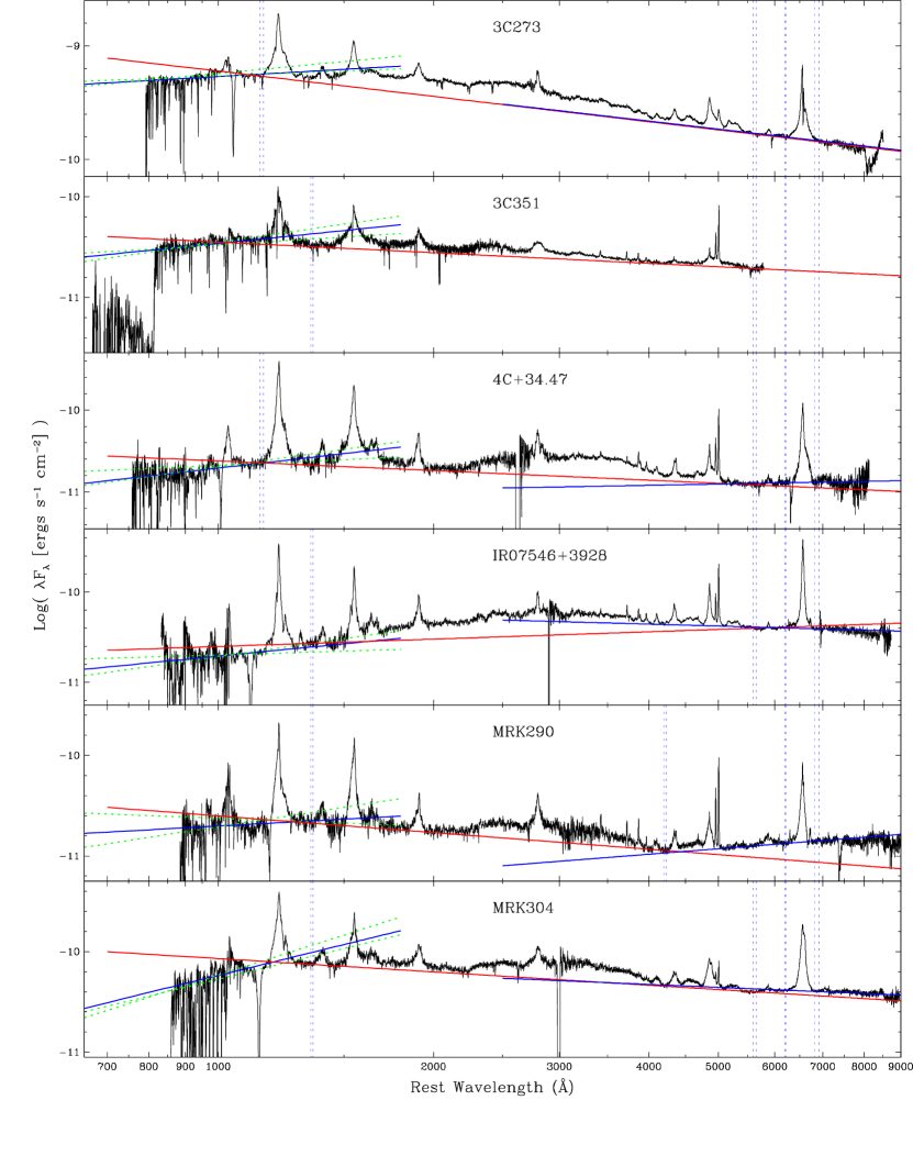
Figure 1: FUV to optical SEDs and fitted power-laws for different regions. Uncertainties in the FUV power-law fitting are also shown. The vertical dotted lines indicate the continuum windows used for fitting $\alpha_{{UVO}}$ ($\sim$1200–5500Å) and $\alpha_{{Ored}}$ ($\sim$5500–9000Å) (Table 3). FUSE spectra have been rebinned to a resolution of 0.5Å for display purpose.

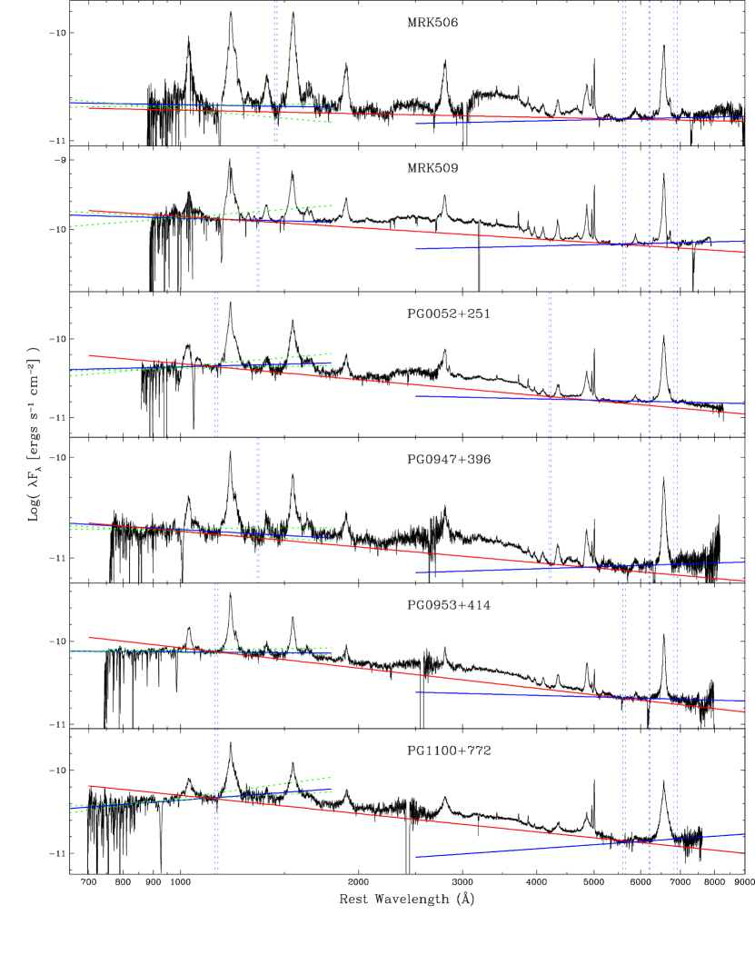
Figure 1: Continued

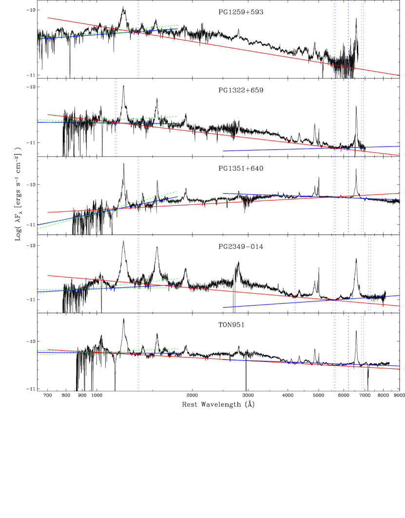
Figure 1: Continued

4 SED ANALYSIS

4.1 SED Measurements

For many objects, the FUV and NUV-optical spectral regions have different slopes (Fig. 1). After careful examination, we decided to use three power-laws to fit the entire FUV-optical continuum.

A power-law with spectral index of $\alpha_{FUV}$ is fitted to the FUV spectral region ( $\lesssim$1100Å) on a case-by-case basis. We first exclude the obvious emission-line regions (Ly$\gamma$ $\lambda$973, C iii $\lambda$977, N iii $\lambda$991, Ly$\beta$ $\lambda$1026, O vi $\lambda$1034, Si iv $\lambda$1062, Si iv $\lambda$1073, and He ii $\lambda$1084, etc.) Strong ISM Lyman series absorption lines and possible AGN O vi and ${\rm Ly}{\alpha}$ absorption features are also excluded. We make sure the excluded regions are wide enough by visual inspection so that the line wings are also excluded. We then fit the remaining data points with a power-law, and iteratively reject points beyond $\pm 2\sigma$ and the points next to the rejected points. This process removes the numerous narrow Galactic H₂ absorption lines and possible residual emission features from the fitting. Finally, we visually inspect the fitting results and make sure that the power-law goes through the apparent continuum regions in the FUV spectra. We repeat this process to estimate upper and lower limits for $\alpha_{FUV}$ by intentionally including some emission or absorption features until the fitted power-law obviously deviates from the spectra (visual inspection). We therefore obtain conservative uncertainties for the best-fit power-law. The fitted $\alpha_{FUV}$ and its uncertainties are listed in Table 3. If there are possible residual weak blended Galactic absorption lines or emission features, they are only comparable with the noise level, and the uncertainty in the fitted spectra indices caused by these weak features is much smaller than the above estimated uncertainties.

Table 3: Spectral Indexes

	FUV		Cont. Windows	1200–5500Å			5500–9000Å				0.1–2.4 keV
Object	$f_{1000}$	$\alpha_{FUV}$	a b c d e f	$f_{1000}$	$\alpha_{{UVO}}$		$f_{1000}$	$\alpha_{{Ored}}$	$\Delta\alpha$	$\lambda_{break}$	$f_{\rm 1kev}$	$\alpha_{\rm x}$
3C273	53.70	$-0.64^{+0.24}_{-0.11}$	x string string x x x	60.00	$-$1.74		60.00	$-$1.73	1.10	$1105^{+0}_{-69}$	283.0	$-1.11^{+0.01}_{-0.01}$
3C351	3.44	$-0.28^{+0.30}_{-0.28}$	string x string x x x	4.69	$-$1.35		$\cdots$	$\cdots$	1.07	$1027^{+57}_{-25}$	3.1	$-1.31^{+0.05}_{-0.05}$
4C+34.47	1.95	$0.00^{+0.21}_{-0.61}$	x string string x x x	2.39	$-$1.39		0.97	$-$0.84	1.39	$1155^{+16}_{-45}$	66.3	$-1.29^{+0.06}_{-0.06}$
IRAS F07546…	1.95	$-0.22^{+0.35}_{-0.54}$	string x string x x x	2.50	$-$0.73		5.99	$-$1.22	0.51	$1620^{+1619}_{-266}$	6.9	$-2.16^{+0.38}_{-0.38}$
MRK290	1.99	$-0.61^{+0.70}_{-0.66}$	string x x string x x	2.50	$-$1.55		0.48	$-$0.44	0.94	$1281^{+69}_{-118}$	30.1	$-1.32^{+0.13}_{-0.13}$
MRK304	5.78	$0.75^{+0.52}_{-0.01}$	string x string x x x	8.52	$-$1.44		7.15	$-$1.30	2.18	$1193^{+49}_{-43}$	$\cdots$	$\cdots$
MRK506	2.15	$-1.09^{+0.16}_{-0.38}$	- string string x x x	1.92	$-$1.11		1.29	$-$0.88	0.02	$\cdots$	26.6	$-1.20^{+0.09}_{-0.09}$
MRK509	14.50	$-1.23^{+0.91}_{-0.23}$	string x string x x x	15.30	$-$1.54		4.32	$-$0.80	0.31	$1201^{+358}_{-167}$	386.0	$-1.61^{+0.03}_{-0.03}$
PG0052+251	4.41	$-0.81^{+0.45}_{-0.04}$	x string x string x x	4.84	$-$1.67		2.19	$-$1.17	0.86	$1111^{+78}_{-48}$	46.2	$-1.49^{+0.02}_{-0.04}$
PG0947+396	1.92	$-1.33^{+0.37}_{-0.02}$	string x x string x x	1.84	$-$1.52		0.60	$-$0.81	0.19	$\phantom{0}813^{+323}_{-87}$	14.9	$-1.18^{+0.18}_{-0.15}$
PG0953+414	7.43	$-1.05^{+0.13}_{-0.04}$	x string string x x x	8.35	$-$1.81		2.91	$-$1.19	0.76	$1165^{+39}_{-100}$	17.0	$-1.43^{+0.03}_{-0.05}$
PG1100+772	4.38	$-0.47^{+0.44}_{-0.14}$	x string string x x x	4.99	$-$1.73		0.57	$-$0.50	1.26	$1114^{+10}_{-72}$	12.5	$-1.56^{+0.08}_{-0.10}$
PG1259+593	4.17	$-0.64^{+0.11}_{-0.12}$	string x string x x x	5.72	$-$1.80		$\cdots$	$\cdots$	1.16	$1313^{+1}_{-93}$	$\cdots$	$\cdots$
PG1322+659	2.26	$-1.06^{+0.31}_{-0.14}$	x string string x x x	2.51	$-$1.66		0.62	$-$0.85	0.60	$1191^{+36}_{-196}$	17.8	$-1.75^{+0.04}_{-0.03}$
PG1351+640	1.96	$0.60^{+0.51}_{-0.20}$	string x string x x x	2.35	$-$0.57		7.80	$-$1.28	1.17	$1173^{+101}_{-62}$	4.2	$-1.43^{+0.06}_{-0.06}$
PG2349-014	1.57	$-0.70^{+0.31}_{-0.22}$	string x x string - -	2.32	$-$1.51		0.49	$-$0.60	0.81	$1616^{+292}_{-284}$	31.2	$-1.44^{+0.12}_{-0.12}$
TON951	5.74	$-1.05^{+0.33}_{-0.27}$	string x string x x x	5.86	$-$1.37		5.12	$-$1.24	0.32	$1066^{+880}_{-77}$	3.2	$-1.54^{+0.11}_{-0.12}$

A single power-law cannot fit the entire NUV-optical region in many objects. This was noticed before, for example, in the Sloan Digital Sky Survey (SDSS) composite spectra (Vanden Berk et al., 2001). Clean continuum regions are also hard to find in the AGN NUV-optical spectra due to the large number of broad emission lines and blends, including the “small blue bump” from $\sim$2000–4000Å— the blend of Fe ii emission and Balmer continuum. We therefore have to define, for this sample, some common, narrow continuum windows where there seem to be no emission lines: 1144–1157Å, 1348–1358Å, 4200–4230Å, 5600–5648Å, 6198–6215Å, and 6820–6920Å.

The NUV-optical spectra index $\alpha_{{UVO}}$ in $\sim$1200–5500Å, and red optical spectra index $\alpha_{{Ored}}$ in $\sim$5500–9000Å are each obtained by fitting a power-law to a pair of selected continuum windows, requiring that all emission features are above the fitted power-laws in the corresponding regions. The continuum windows used for each object are listed in Table 3 and marked in Figure 1. Since the continuum windows are very narrow, this fitting process is more like defining each power-law with two points. The power laws cannot be treated as the true continua of the spectra, but the spectral indices provide information on the overall continuum slopes.

The UV bump can now be characterized with two power-laws (a broken power-law) with spectral indices of $\alpha_{FUV}$ and $\alpha_{{UVO}}$, and a break wavelength $\lambda_{break}$, which is defined by the intersection of the two power-laws.

4.2 Spectral Break in SEDs

As can be seen in Figure 1, an extrapolation of the NUV-optical power-law does not match the FUV continuum in most objects. For the possible exceptions, Mrk 290, Mrk 506, Mrk 509, PG0947+396, and Ton 951, the extrapolated NUV-optical power-law falls within the bounds of the errors for our fits to the FUV continuum. Thus, for 12 out of 17 objects, we see a break in the spectral index to a steeper value when comparing the NUV-optical to the FUV continuum.

The break wavelength is calculated as the intersection point of the two power-laws. The distribution of the break wavelength is shown in Figure 2, where $\lambda_{break}$ peaks near 1100Å and spans 800–1600Å. However, since the calculated break wavelength is very sensitive to small changes in $\alpha_{FUV}$ or $\alpha_{{UVO}}$ when the difference between $\alpha_{FUV}$ and $\alpha_{{UVO}}$ is small, it has a large uncertainty for some objects (Table 3).

Figure 2: Distribution of the break wavelength, indicating a spectral break near 1100Å for most objects. The largest $\lambda_{break}$ is from IRAS F07546+3928 (§4.2) and PG2349-014. Mrk506 does not show a spectral break and is not included.

We have also compared our SEDs with the soft X-ray spectral indices in Figure 3 in a similar way as in Laor et al. (1997), except that we also have FUV data. For more than half our objects, the soft X-ray spectral indices appear to match up reasonably with the extrapolation of the FUV continuum. This directly confirms the finding by Laor et al. (1997) and Zheng et al. (1997) in composite spectra that the peak of the big blue bump lies in the FUV region.

Three objects, IRAS F07546+3928, NGC 3516, and PG1351+640, show strongly suppressed NUV-FUV continua. These objects also show intrinsic absorption features, possibly suggesting the existence of dust associated with the absorbers. (See Zheng et al. (2001) for the case of PG 1351+640.) We will discuss the reddening effect more in §6.

Figure 3: FUV-optical SEDs and the soft X-ray spectral indices. The dotted lines are drawn to connect FUV spectra and X-ray spectral slopes, and the dashed lines indicate the extrapolation of fitted FUV power-law. More than half of the objects have an X-ray spectral slope roughly matching the extrapolation of the FUV continuum slope. Also note the large UV suppression of IRAS F07546+3928, NGC 3516, and PG1351+640.

4.3 Bolometric Luminosity

Bolometric luminosity ($L_{Bol}$) is one of the most fundamental parameters for understanding the black hole accretion in quasars, however, it has not been easy to obtain for quasars in general, because they emit significant power over a large part of the electromagnetic spectrum.

Elvis et al. (1994) built SEDs for a sample of 47 quasars and were able to obtain the bolometric luminosity by integrating over the SEDs from radio to X-ray wavelengths. They also determined the bolometric correction factors for a few monochromatic luminosities, e.g., $L_{Bol}\approx 13\lambda L_{\lambda}$(5400Å), based on their SEDs. Different empirical correction factors have been determined and used to estimate $L_{Bol}$ in previous studies (e.g., Sanders et al., 1989; Laor & Draine, 1993; Wandel, Peterson, & Malkan, 1999). Recently, many studies use the prescription of Kaspi et al. (2000) to estimate quasar black hole masses and bolometric luminosity $L_{Bol}=9\lambda L_{\lambda}$(5100Å).

Since we have broad spectral coverage from the FUV to optical, we are able to obtain an accurate luminosity for this region by integrating over the power-laws we measure. To estimate the bolometric luminosity, we need to include X-ray and IR regions. We extend our FUV power-law continuum to 700Å, and then use a power-law to connect with the soft X-ray luminosity at 0.2 keV.

The case for the infrared region is more complicated. There is an IR bump around 10µm in quasar SEDs, which also contributes a significant amount of energy. After averaging the mean SEDs for radio-loud and radio-quiet objects from Elvis et al. (1994), we fit two power-laws to characterize this bump and obtain ${\alpha_{\lambda}}=-0.69$ for 1–10µm and ${\alpha_{\lambda}}=-1.65$ for 10–100µm. These two power-laws form a peak at 11.45µm, roughly corresponding to the peak in the mean SEDs. We scale this power-law IR bump to match the extrapolation of the fitted NUV-optical continuum at 1µm for each object.

We estimate the bolometric luminosity between 2 keV and 100µm by integrating this set of power-laws over this region. We have also obtained the luminosities for individual wavebands. Table 4 lists the results.

Table 4: Integral Bolometric and Individual Waveband Luminosities

Object	$L_{X}$	$L_{XFUV}$	$L_{FUVO}$			$L_{IR}$			$L_{Bol}$
			case A	case B		case A	case B		case A	RA	case B	RB
3C273	45.51	46.22	46.51	46.51		46.42	46.41		46.94	1.48	46.94	1.47
3C351	44.23	45.44	$\cdots$	46.04		$\cdots$	46.20		$\cdots$	$\cdots$	46.50	1.03
4C+34.47	45.13	45.30	45.42	45.41		45.72	45.56		46.07	1.62	46.00	1.39
IR07546+3928	43.83	44.54	45.09	45.11		45.53	45.64		45.72	0.98	45.80	1.17
MRK290	43.23	43.64	43.86	43.81		44.26	43.86		44.52	1.83	44.34	1.20
MRK304	$\cdots$	$\cdots$	45.02	45.01		45.22	45.16		45.46	1.08	45.42	0.99
MRK506	43.44	43.95	44.20	44.19		44.54	44.48		44.81	1.39	44.78	1.29
MRK509	44.53	44.87	44.75	44.74		44.96	44.77		45.44	2.28	45.38	1.99
PG0052+251	44.81	45.33	45.43	45.42		45.53	45.37		45.98	1.83	45.93	1.62
PG0947+396	44.45	45.11	45.31	45.29		45.54	45.32		45.86	1.71	45.76	1.36
PG0953+414	44.67	45.66	45.94	45.94		45.94	45.78		46.41	1.72	46.35	1.53
PG1100+772	44.78	45.63	45.95	45.93		46.13	45.85		46.47	1.79	46.36	1.37
PG1259+593	$\cdots$	$\cdots$	$\cdots$	46.24		$\cdots$	46.13		$\cdots$	$\cdots$	46.57	1.09
PG1322+659	44.54	45.16	45.22	45.21		45.36	45.16		45.80	1.93	45.73	1.66
PG1351+640	43.30	44.13	45.08	45.11		45.52	45.71		45.68	0.83	45.83	1.16
PG2349-014	44.71	45.07	45.22	45.20		45.54	45.30		45.87	1.82	45.77	1.45
TON951	42.95	44.39	44.92	44.90		45.12	45.05		45.41	1.26	45.37	1.15

Note. — Values are the logarithm of luminosity in units of $\mbox{ergs s}^{-1}$. $L_{X}$: 2–0.2 keV; $L_{XFUV}$: 0.2 keV–700Å; $L_{FUVO}$: 700Å–1µm; $L_{IR}$: 1µm–100µm; $L_{Bol}$: 2 keV–100µm.

Since we do not use actual measurements in the IR (few exist for our sample objects), we scale the IR bump in two ways so that we have a range of the estimated IR luminosity. In case A, we match the IR bump with the extrapolation of the red optical power-law of $\alpha_{{Ored}}$ at 1µm; in case B, we ignore $\alpha_{{Ored}}$ and use NUV-optical power-law of $\alpha_{{UVO}}$ for the entire optical region, and match the IR bump with the extrapolation of $\alpha_{{UVO}}$ at 1µm. Therefore, we have two integral luminosities for FUV-optical $L_{FUVO}$ (700Å–1µm), two estimated luminosities of the IR bump $L_{IR}$ (1–100µm), and two estimates of $L_{Bol}$ (2 keV–100µm). These two cases give consistent results for $L_{FUVO}$, but result in a big difference, up to a factor of 2.5 in $L_{IR}$, when $\alpha_{{UVO}}$ and $\alpha_{{Ored}}$ are significantly different. In any case, $L_{IR}$ is comparable with $L_{FUVO}$ and contributes significantly to $L_{Bol}$. Table 5 shows the comparison between $L_{IR}$ and $L_{FUVO}$. The distribution of $L_{IR}$/$L_{FUVO}$ has a large dispersion, in general agreement with the data of Elvis et al. (1994).

Table 5: Statistics of $L_{IR}$/$L_{FUVO}$

	Median	Mean	Min	Max
Case A	1.61	1.76 $\pm$0.63	0.78	2.78
Case B	1.20	1.49 $\pm$0.91	0.70	4.00
Elvis et al. (1994)	1.17	1.56 $\pm$1.23	0.58	5.89

Figure 4 compares our integral $L_{Bol}$ with the bolometric luminosity estimated using the empirical formula from a monochromatic optical luminosity, $L_{Bol}=9\lambda L_{\lambda}$(5100Å). The ratios of $L_{Bol}$/9$\lambda L_{\lambda}$(5100Å) are listed in Table 4. (The $\lambda L_{\lambda}$(5100Å) is measured in a local continuum. See §4.4). There exists a strong correlation between the integral $L_{Bol}$ and 9$\lambda L_{\lambda}$(5100Å), but our results are 30–70% ($\sim 0.1-0.2$ dex) larger in general and seems to agree better with the correction factor determined by Elvis et al. (1994). These imply that the bolometric correction factor may be larger than 9, and more like 13 for using $\lambda L_{\lambda}$(5100Å).

Figure 4: Comparison between integral $L_{Bol}$ and 9$\lambda L_{\lambda}$(5100Å). The solid line indicates $L_{Bol}=1.5\times 9\lambda L_{\lambda}(5100\mbox{\AA})$, it is not a least square fit.

Although we obtain accurate FUV-to-optical luminosities from our SEDs, a few sources contribute to the uncertainties of the integral bolometric luminosity. First, Elvis et al. (1994) warned about the use of mean SEDs, because the shapes of SEDs in individual objects have large dispersion. Second, our scaling of the IR bump may cause large uncertainties since we use simple extrapolations of the NUV-optical and red optical power-laws. We have seen a difference of 30% (0.1 dex) in $L_{Bol}$ for case A and B. Third, we have no data for $L_{XFUV}$, and the cutoff wavelength of 700Å for $L_{FUV}$ is chosen subjectively. Finally, the X-ray data were not obtained simultaneously with our FUV-optical spectra, and the X-ray variability is another source of uncertainty. These should be kept in mind when interpreting our integral $L_{Bol}$.

For simplicity and easy comparison with other work, we will use $L_{Bol}$=9$\lambda L_{\lambda}$(5100Å) for the bolometric luminosity in the rest of the paper. This choice does not change any statistical significance in analyses involving $L_{Bol}$, and it is easy to compare with our integral bolometric luminosity by using Table 4 to correct for individual objects.

4.4 Estimation of Black Hole Mass

We have estimated the black hole mass and accretion rate using a recently developed method based on reverberation mapping of the broad-line region (BLR) and on the assumption of virial motion (Kaspi et al., 2000),

$$M_{BH}=R_{BLR}\ v^{2}/G.$$ (1)

${\rm H}{\beta}$ is used for estimating the velocity dispersion, $v=\sqrt{3}/2$ FWHM(${\rm H}{\beta}$), and $R_{BLR}$ is the size of the broad line region and can be estimated empirically from reverberation mapping studies (Kaspi et al., 2000),

$$R_{BLR}=32.9^{+2.0}_{-1.9}\left[\frac{\lambda L_{\lambda}(5100\mbox{\AA})}{10^{44}\mbox{erg s}^{-1}}\right]^{0.70\pm 0.033}\mbox{ light days}.$$ (2)

We use the bolometric luminosity $L_{bol}=9\lambda L_{\lambda}(5100\mbox{\AA})$. Given the black hole mass and bolometric luminosity, we can also estimate the Eddington ratio, $L/L_{Edd}$.

We measure the FWHM(${\rm H}{\beta}$) by fitting the ${\rm H}{\beta}$ region with the IRAF task specfit (Kriss, 1994). A local power-law continuum, the [O iii] lines, and He ii $\lambda$4686 are also fitted together with ${\rm H}{\beta}$ (Fig. 5). We use a broad and a narrow Gaussian component to fit the ${\rm H}{\beta}$ broad line, and allow a relative wavelength shift between the two components to account for the ${\rm H}{\beta}$ asymmetry. A narrow-line-region (NLR) component of ${\rm H}{\beta}$ is also introduced, but it is often negligible. Both the width and the wavelength of this NLR component are tied with those of [O iii] $\lambda$5007. The intensity ratio of [O iii] $\lambda$5007/$\lambda$4959 is assumed to be 3:1 based on their statistical weights. A single Gaussian profile is fitted for each of [O iii] $\lambda\lambda$4959,5007.

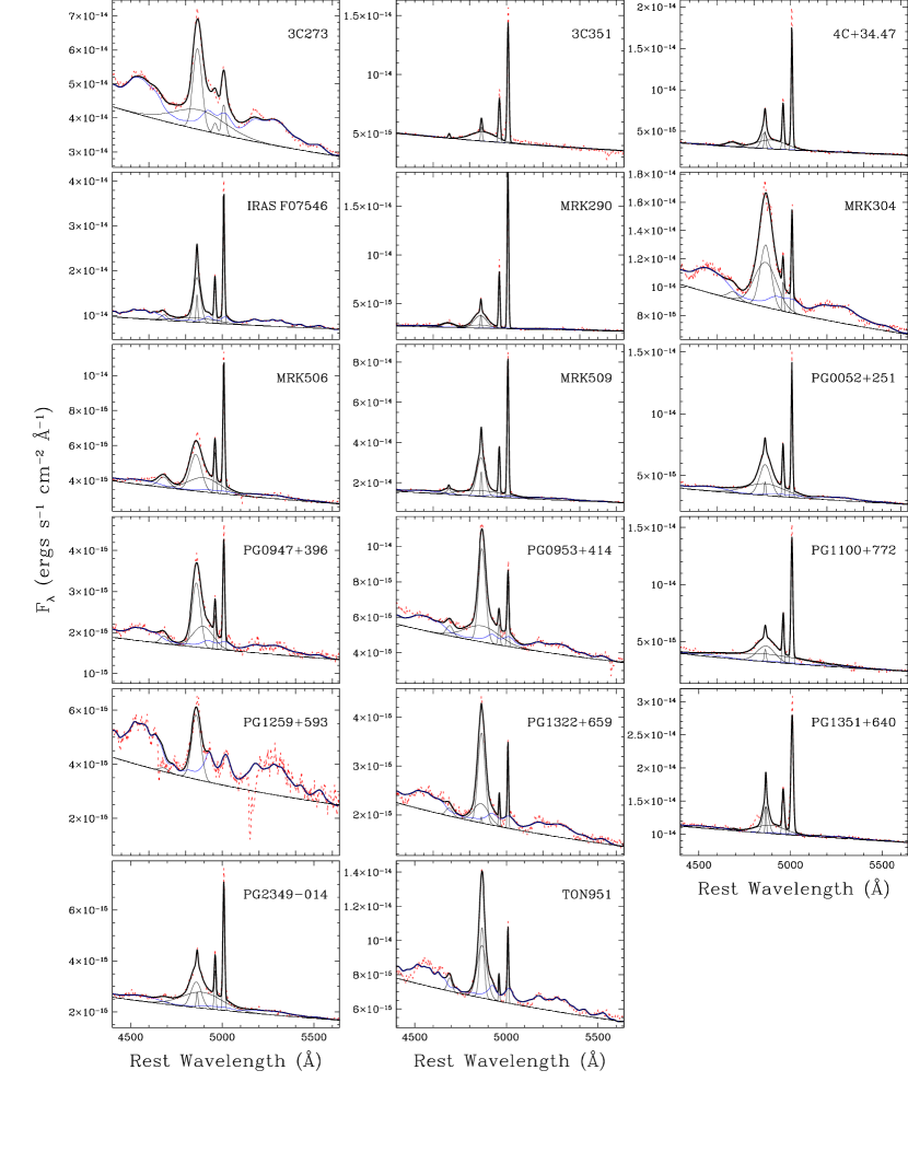
Figure 5: Model fitting to the ${\rm H}{\beta}$ region. The dotted lines show the data, and the thick solid lines the fitting results. Also shown are the local continua, Fe ii template, and individual components of ${\rm H}{\beta}$, [O iii], and He ii $\lambda$4686.

Broad Fe ii emission blends are often strong in this region, especially when [O iii] is weak. In order to remove the Fe ii contamination, we use an Fe ii template from Boroson & Green (1992). The strength of the Fe ii template is free to vary in the fitting process, and it is also broadened to be consistent with FWHM(${\rm H}{\beta}$) for each object.

We calculate the final FWHM(${\rm H}{\beta}$) from the fitted ${\rm H}{\beta}$ model profiles. Specifically, we exclude the NLR component, and use the other two fitted Gaussian components, taking into account the relative wavelength shift between these two components. The uncertainty of FWHM(${\rm H}{\beta}$) is less than 10%.

The rest-frame reference is defined with [O iii]$\lambda$5006.8, and the fitted wavelength of [O iii] $\lambda$5007 is used to calculate the redshift. The uncertainty of the redshift is $<0.0002$ for all objects except for PG1259+592, which has very weak [O iii], and has a redshift uncertainty of 0.002.

Table 6 lists the fitting results, together with calculated $M_{BH}$ and $L/L_{Edd}$ etc. Six objects in our sample also have black hole masses derived from reverberation mapping studies (Kaspi et al 2000). They are also listed in the table. Our results are usually larger, because we have excluded the ${\rm H}{\beta}$ NLR component when obtaining the FWHM(${\rm H}{\beta}$). Therefore we have a larger FWHM(${\rm H}{\beta}$) and hence a larger $M_{BH}$. As was also noticed by Boroson (2002) and Vestergaard (2002), 3C351 (i.e., PG 1704+608) is an extreme case, in which the very narrow ${\rm H}{\beta}$ component on top of the broad ${\rm H}{\beta}$ emission is identified as an NLR component with the same width as [O iii] (690 ${\rm km~{}s}^{-1}$). It is excluded from calculating FWHM(${\rm H}{\beta}$) in our study, but not in Kaspi et al. (2000). This results in a huge difference in FWHM(${\rm H}{\beta}$) and hence in $M_{BH}$.

Another uncertainty of the FWHM(${\rm H}{\beta}$) comes from the uncertainty of the fitted local continuum level. Assuming a single Gaussian profile, if the continuum is lowered by 10% of the line peak, the estimated FWHM will increase by $\sim$ 7%, and the calculated black hole mass from FWHM(${\rm H}{\beta}$) and the continuum luminosity based on Eq.1 and 2 will increase by 7%.

On the other hand, sometimes we had to scale the optical spectra to match the HST NUV spectra due to likely source variability. A scaling of 30% can change the estimated black hole mass by 20%. The AGN intrinsic variability can also change the emission-line profile, and hence the estimated black hole mass. Different approaches for spectral measurements in different studies can lead to large discrepancies in reported masses. Due to all the above reasons, the estimated black hole mass from different studies can easily differ by a factor of a few, in our case, a maximum factor of 5 for 3C273 (excluding the extreme case of 3C351). In fact, Vestergaard (2002) compared the black hole masses estimated from reverberation mapping and from single-epoch optical observation, and concluded that they agree within factors of 3, 6, and 10 with probabilities of 80%, 90%, and 95%, respectively. However, if one keeps consistency in measurements and calculation for a sample, the relative uncertainty in the estimated black hole masses within the sample should be much smaller.

Table 6: Black Hole Mass and Eddington Ratio

Object	z	FWHM(${\rm H}{\beta}$)	$f_{\lambda}$(5100Å)	$\lambda L_{\lambda}$(5100Å)	$M_{BH}$	$L/L_{Edd}$	$M_{BH}$(rev)
		(${\rm km~{}s}^{-1}$)	(erg s-1 cm-2 Å-1)	log(erg s-1)	($10^{8}M\sun$)		($10^{8}M\sun$)
3C273	0.1576	4115	3.41E-14	45.82	11.50	0.41	2.35
3C351	0.3730	9760	4.11E-15	45.54	41.18	0.06	0.075
4C+34.47	0.2055	3520	2.64E-15	44.91	1.94	0.30
IR07546+3928	0.0953	2965	7.89E-15	44.78	1.12	0.39
MRK290	0.0303	5505	2.38E-15	43.31	0.36	0.04
MRK304	0.0657	5570	7.96E-15	44.48	2.43	0.09
MRK506	0.0428	5520	3.15E-15	43.72	0.70	0.05
MRK509	0.0345	3630	1.22E-14	44.13	0.59	0.16	0.92
PG0052+251	0.1544	5465	3.12E-15	44.77	3.73	0.11	3.02
PG0947+396	0.2057	3810	1.53E-15	44.68	1.57	0.22
PG0953+414	0.2338	3155	4.23E-15	45.22	2.57	0.46	1.64
PG1100+772	0.3114	9300	2.94E-15	45.27	24.20	0.06
PG1259+593	0.4769	3615	3.11E-15	45.58	6.03	0.45
PG1322+659	0.1684	3030	1.67E-15	44.56	0.82	0.32
PG1351+640	0.0882	2840	9.69E-15	44.81	1.08	0.43	0.30
PG2349$-$014	0.1740	5900	1.98E-15	44.66	3.64	0.09
TON951	0.0643	2390	6.19E-15	44.36	0.37	0.45

4.5 Correlation Analyses

It is natural to think that the properties of the UV bump, thought to arise from the accretion disk, are governed by the AGN fundamental parameters, such as $M_{BH}$ and $L/L_{Edd}$. For example, standard thin disk models predict low disk temperatures for high $M_{BH}$ and/or low $L/L_{Edd}$ (Shakura & Sunyaev, 1973) and therefore longer break wavelengths. We looked for such correlations in our sample, but we do not find any significant correlation between the UV bump properties we have measured ($\alpha_{FUV}$, $\alpha_{{UVO}}$, $\Delta\alpha$, and $\lambda_{break}$) and $M_{BH}$, or $L/L_{Edd}$. Table 7 lists the Pearson correlation coefficients for selected parameters. A principal component analysis has also been performed on these parameters, and no hidden correlations are revealed. We also group the objects into subsamples based on $L/L_{Edd}$ (or $M_{BH}$), but there is still no evidence of a correlation within subsamples (see Fig. 6 for an example). However, Scott et al. (2004) found a weak correlation at 96% confidence level between $\alpha_{FUV}$ and $M_{BH}$ in their subsample of 21 AGNs. There are only 4 objects in common between these two studies. The inconsistency between the results most likely arises from the small size of the samples. In any case, the fact that there are no or weak correlations suggests that $M_{BH}$ and $L/L_{Edd}$ are not the only parameters underlying the observed properties of the UV bump. Other factors, such as the disk inclination, intrinsic reddening or other unidentified parameters must also play an important role (§5). We also note that a large spread over $M_{BH}$ and $L/L_{Edd}$ within the small samples may wash out any correlation with spectral index, but our sample is too small to address this.

Table 7: Pearson Correlation Coefficients ($r$)

	log($M_{BH}$)	$L/L_{Edd}$	$\alpha_{FUV}$	$\alpha_{{UVO}}$	$\Delta\alpha$	$\lambda_{break}$	E(B-V)	$\alpha_{\rm x}$
log($M_{BH}$)	1.00
$L/L_{Edd}$	$-$0.16	1.00
$\alpha_{FUV}$	0.23	$-$0.06	1.00
$\alpha_{{UVO}}$	$-$0.33	0.12	0.46	1.00
$\Delta\alpha$	0.47	$-$0.14	0.82	$-$0.13	1.00
$\lambda_{break}$	0.02	0.06	0.34	0.39	0.14	1.00
E(B-V)	$-$0.16	$-$0.24	0.31	0.30	0.15	0.28	1.00
$\alpha_{\rm x}$	0.23	$-$0.24	$-$0.09	$-$0.31	0.15	$-$0.67	$-$0.64	1.00

Note. — 17 objects are used except for $\alpha_{\rm x}$ (15 objects) and $\lambda_{break}$ (16 objects). The chance probability ($p$) of 1%, 2%, and 5% corresponds to a correlation coefficient of 0.61, 0.56, and 0.48, respectively, for 17 objects. Large correlation coefficients marked in bold face do not reveal significant physical correlations (see §4.5 for detail).

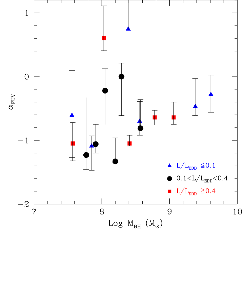
Figure 6: No correlation between $\alpha_{FUV}$ and $M_{BH}$ for the total sample or for subsamples grouped by $L/L_{Edd}$.

A strong correlation ($r=0.82,p=0.0001$) seen in Table 7 is between $\Delta\alpha$ ($=\alpha_{FUV}-\alpha_{{UVO}}$) and $\alpha_{FUV}$. This is simply because the distribution of the NUV-optical spectra index $\alpha_{{UVO}}$ is relatively narrow, while $\alpha_{FUV}$ spans a wide range. Figure 7 shows this clearly. Most objects have $\alpha_{{UVO}}$ between $-2$ and $-1$ with a median value of $-1.52$, but the distribution of $\alpha_{FUV}$  is broader (Fig. 7b).

There seems to be an anti-correlation between $\alpha_{\rm x}$ and $\lambda_{break}$, but there are only 14 objects with values of both $\alpha_{\rm x}$ and $\lambda_{break}$ ($r=-0.67,p=0.01$). Since $\lambda_{break}$ has very large uncertainty, this correlation should not be treated seriously.

We also see a correlation ($r=0.64,p=0.01$, for 15 objects) between E(B-V) and $\alpha_{\rm x}$, but this is largely due to an outlier, IRAS F07546+3928, with the softest ${\alpha_{\rm x}}=-2.16$. Without this outlier, the correlation disappears ($p=0.23$). After careful checking, we find no other correlations that are created or destroyed by outliers.

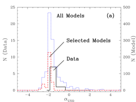
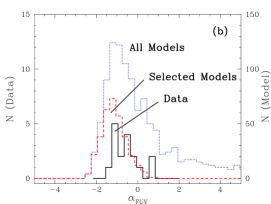
Figure 7: Distributions of $\alpha_{{UVO}}$ and $\alpha_{FUV}$ of the sample (solid line), all models (dotted line, §5) and the selected models (dashed line, $10^{8}M_{\odot}<M_{BH}\leq 4\times 10^{9}M_{\odot}$, $0.03<L/L_{Edd}<0.3$). Note that no selected models are as red as $\alpha_{{UVO}}>-1$. Two reddest objects ($\alpha_{{UVO}}>-1$) are IRAS F07546+3928 and PG 1351+640, both of which show evidence of intrinsic dust reddening.

5 COMPARISON WITH THIN-DISK MODELS

As mentioned above, the expected correlations between the UV bump and $M_{BH}$ or $L/L_{Edd}$ may be mitigated by the small sample size, a large variation in these parameters within the sample, and by other parameters affecting the spectrum of the accretion disk. We used the thin disk model developed by Hubeny et al. (2000) to investigate this.

The models are constructed for a non-LTE disk with 5 free parameters: black hole mass, mass accretion rate ($\dot{M}$), viscosity parameter ${\alpha_{visco}}$, black hole spin, and inclination angle $\cos i$. The total spectrum of a disk is integrated over the individual annuli, taking into account the inclination angle. We have chosen a grid of models with a maximally rotating Kerr black hole with possible values of $M_{BH}$ between $0.125\times 10^{9}$ and $32\times 10^{9}M_{\odot}$, $\dot{M}$ between $2^{-12}M_{\odot}\,{\rm yr}^{-1}$ and $64M_{\odot}\,{\rm yr}^{-1}$, ${\alpha_{visco}}=0.01$ or 0.1, and $\cos i$ between 0.01 and 0.99. The maximum Eddington ratio is limited to $L/L_{Edd}\approx 0.3$. Above this value, the model disk becomes geometrically thick and thus no longer self-consistent.

In order to make statistical comparisons between theory and observation, we have measured $\alpha_{FUV}$, $\alpha_{{UVO}}$, and $\lambda_{break}$ of the models in the same way we have measured them in our data. Figure 8 shows examples of how we measure the model spectra. The Lyman break is prominent in some models, especially when $L/L_{Edd}$ is small. However, due to relativistic boosting and aberration, small $\cos i$ (edge-on) tends to smear out the edges and also shift them to shorter wavelengths. Therefore, to measure $\alpha_{FUV}$ for models with different $\cos i$, we fit a power-law to a different smooth region of $\sim$200Å blueward of the Lyman break. We note that this is not exactly the same as in measuring our data, but this characterizes the UV bump of the models very well except for those with very strong Lyman edges (Fig. 8), and the estimate is consistent for all models with and without a strong Lyman edge. The NUV-optical spectral index is measured the same way as in our real data by fitting a power-law to two continuum windows around 1350Å and 5630Å (continuum windows b and d in Table 3). $\lambda_{break}$ is calculated from $\alpha_{FUV}$ and $\alpha_{{UVO}}$.

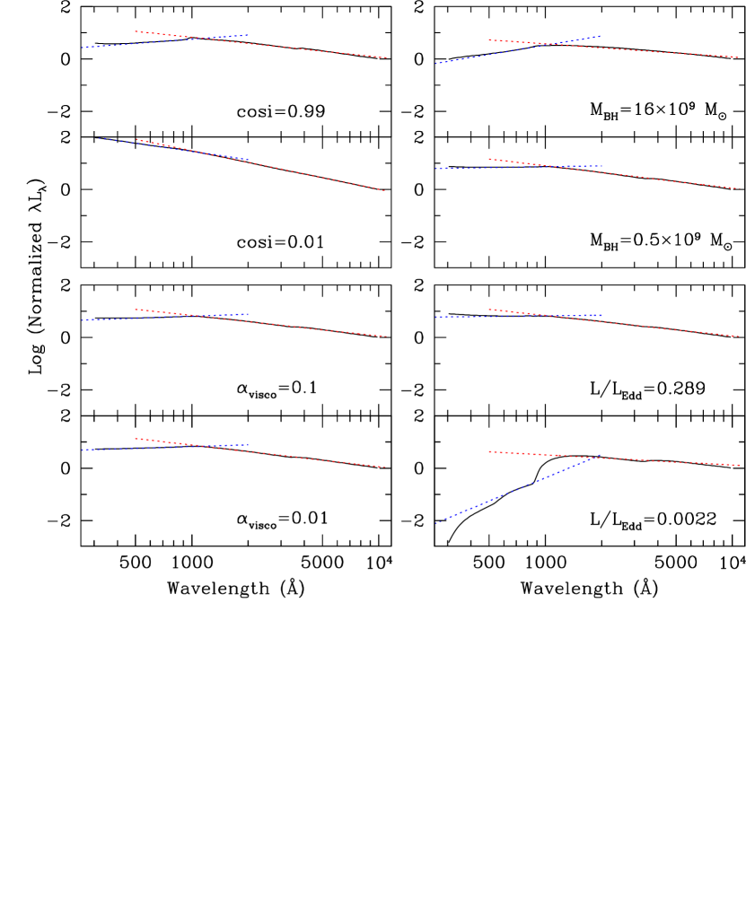
Figure 8: Examples of power-law fitting to the disk model spectra. Solid lines are the model spectra, and dotted lines are the fitted power-laws. Unless marked in each panel, the default model parameters are: $M_{BH}=1\times 10^{9}M_{\odot}$, $L/L_{Edd}=0.145$, ${\alpha_{visco}}=0.1$, and ${\cos i}=0.8$ ($i=37\arcdeg$, close to face-on). Note that FUV slopes obviously change with $M_{BH}$, $L/L_{Edd}$ and $\cos i$ (but not $\alpha_{visco}$), but UV-optical slopes do not change much. Also note the strong Lyman break in the spectrum with low $L/L_{Edd}$ (0.0022).

Similar to our data, the distribution of $\alpha_{{UVO}}$ measured from all the models is relatively narrow with a median value of $-1.74$. We further select only models with similar black hole masses ($M_{BH}\sim 10^{8}-4\times 10^{9}M_{\odot}$) and Eddington ratios ($L/L_{Edd}\sim 0.03-0.3$) to those of our sample and compare them with our data (Fig. 7a). The $\alpha_{{UVO}}$ of the selected models has a median value of $-1.91$ (standard deviation $\sigma=0.26$), roughly in agreement with our data (median $\alpha_{{UVO}}=-1.52$, $\sigma=0.35$). While there are no selected models that are as red as $\alpha_{{UVO}}>-1$ (Fig. 7a), two objects, IRAS F07546+3928 and PG 1351+640, are redder than $\alpha_{{UVO}}>-1$, but both show obvious evidence of dust reddening. We note that 7 objects in our sample have $L/L_{Edd}>0.3$, and 5 objects have $M_{BH}<10^{8}M_{\odot}$, and these values of the parameters have not been covered by our current models. Examining the model trends in Figure 3 of Blaes (2004), extrapolating $L/L_{Edd}$ of the models to 0.5 would probably not change $\alpha_{UVO}$ by more than 0.1. However, lower black hole masses result in smaller (bluer) $\alpha_{UVO}$ in the models, and such values are not seen in the data. On the other hand, we have assumed a near maximal black hole spin in all the models used here. Lower black hole spins generally increase $\alpha_{UVO}$ in the models, and would improve agreement with the data. It would therefore be worth exploring such low spin models in the future.

$\alpha_{FUV}$ from the models still has a broad distribution, also in agreement with our data (Fig. 7b). Since the distribution of $\alpha_{{UVO}}$ is narrow, the spectral breaks at the UV bump ($\lambda_{break}$ and ${\Delta\alpha}\ =\alpha_{FUV}-\alpha_{{UVO}}$) are mainly defined by the change of FUV spectral index $\alpha_{FUV}$ in both our data and the models. $\alpha_{FUV}$ is sensitive to $M_{BH}$, $L/L_{Edd}$, and $\cos i$, but not to the viscosity parameter ${\alpha_{visco}}$, as shown in Figure 8.

We further compare our data with the models by showing the changes of $\alpha_{FUV}$, $\Delta\alpha$ and $\lambda_{break}$ with $M_{BH}$ and $L/L_{Edd}$ (Fig. 9 and 10). We chose the models for extreme face-on ($\cos i$=0.99) and extreme edge-on ($\cos i$=0.01) cases with ${\alpha_{visco}}=0.1$.

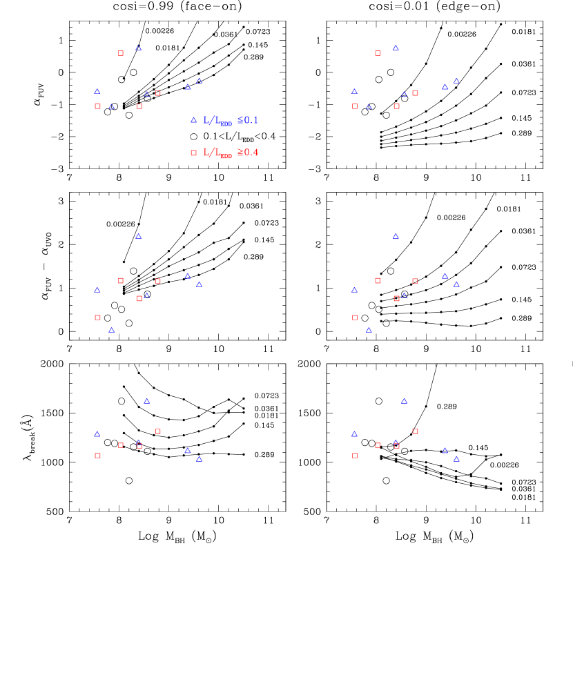
Figure 9: Properties of the spectral break vs. black hole mass for both data and model predictions (face-on and edge-on). The different open symbols are for the individual objects in different $L/L_{Edd}$ ranges. The solid lines are the model predictions. $L/L_{Edd}$ for each line is marked with a number close to the lines. The irregular patterns (intersections) of the models in the lower panels are due to the uncertainty of calculated $\lambda_{break}$, which is mainly from the way we measure $\alpha_{FUV}$ in models with strong Lyman edge (see text).

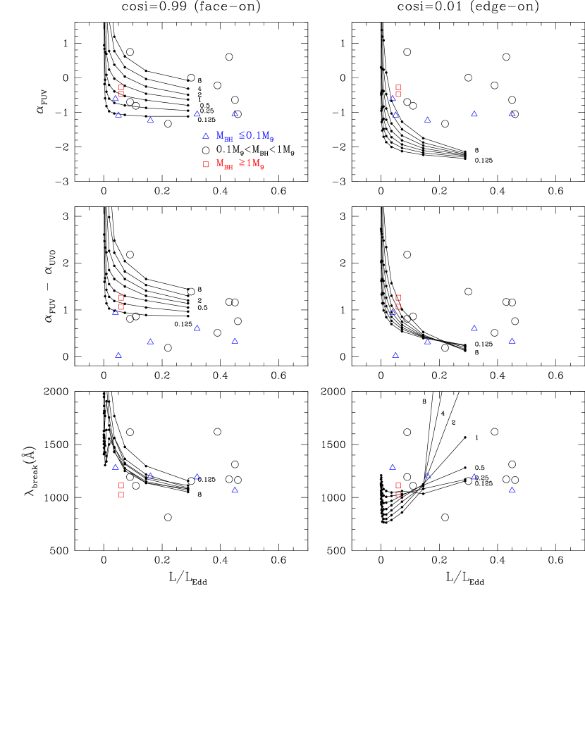
Figure 10: Properties of the spectral break vs. Eddington ratio for both data and model predictions (face-on and edge-on). The different open symbols are for the individual objects in different $M_{BH}$ ranges. The solid lines are the model predictions. $M_{BH}$ for each line is marked with a number close to the lines in units of $M_{9}$ ($M_{9}=10^{9}M_{\odot}$).

In the face-on models, there is a clear correlation between $\alpha_{FUV}$ (hence $\Delta\alpha$) and $M_{BH}$ for $L/L_{Edd}\approx 0.01-0.3$ (Fig. 9, top-left). However, no evidence of such a trend can be seen in our data, even when we group the objects into subsamples of narrower $L/L_{Edd}$ ranges. Moreover, the models do not cover the $\alpha_{FUV}$-$M_{BH}$ space with enough overlap of the data except for extremely small $L/L_{Edd}$, but these small $L/L_{Edd}$ are not seen for for our AGNs. Some AGNs seems to follow the model prediction in one plot (2-dimensional space), but they do not match the same model prediction in other plots (other dimensions). Although we do not have information on the inclinations of objects in our sample, large disk inclinations only increase the discrepancy (Fig. 9, top-right). We will discuss this inconsistency more in §6.

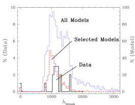
Figure 11: Distribution of $\lambda_{break}$ of the sample (solid line), all models (dotted line), and the selected models (dashed line, $10^{8}M_{\odot}<M_{BH}\leq 4\times 10^{9}M_{\odot}$, $0.03<L/L_{Edd}<0.3$). Note the peak for the models is around 1000Å. The second bump between 1200–1400Å for all models is due to an overestimate for models with a strong Lyman edge.

$\lambda_{break}$ does not seem to correlate with $M_{BH}$ (Fig. 9, bottom-right). For large $L/L_{Edd}$ in face-on cases, $\lambda_{break}$ is close to 1000Å, but for smaller $L/L_{Edd}$, $\lambda_{break}$ goes to longer wavelengths. This is because $\alpha_{FUV}$ is underestimated for models with a strong Lyman edge, as can be seen in Figure 8 (bottom-right). The distribution of model $\lambda_{break}$ also shows this clearly (Fig. 11). While there is a peak around 1000Å in the histogram, there is also a second bump between 1200–1400Å which accounts for the models with a strong Lyman edge. This bump disappears in the case of the selected models, where models with small $L/L_{Edd}$ (strong Lyman edge) are excluded. In the edge-on cases (Fig. 9, bottom-right), large inclination causes strong relativistic effects which smear out the Lyman edge, bringing the measured $\lambda_{break}$ back to around 1000Å. The extremely large values of $\lambda_{break}$ for $L/L_{Edd}$=0.289 simply indicate that there is not a clear spectral break, because $\alpha_{FUV}\approx\alpha_{{UVO}}$.

We have also plotted $\alpha_{FUV}$, $\Delta\alpha$, and $\lambda_{break}$ against $L/L_{Edd}$ for different $M_{BH}$ (Fig. 10). No clear correlation is seen. If we could extend $L/L_{Edd}$ of the models to above 0.3, the models seem to cover a region that overlaps with our data points (face-on), but the $M_{BH}$ required for the models needs to extend above $10^{9}M_{\odot}$, much higher than those calculated for most of our AGNs. The apparent correlation seen in $\lambda_{break}$-$L/L_{Edd}$ is largely biased by models with small $L/L_{Edd}$, for which $\lambda_{break}$ is overestimated due to the strong Lyman edge.

Large inclination angle (small $\cos i$, edge-on) has several effects on the models: (1) it decreases (flattens) $\alpha_{FUV}$, weakening the correlation between $\alpha_{FUV}$ and $M_{BH}$ seen in face-on models (Fig. 9, top-left); (2) it results in smaller difference between $\alpha_{FUV}$ and $\alpha_{{UVO}}$  and tends to smear out the UV bump ($\alpha_{FUV}\approx\alpha_{{UVO}}$), resulting in unrealistically large (or small) $\lambda_{break}$ (Fig. 9, bottom-right); (3) it forces the models to a narrow region in $\alpha_{FUV}$-$L/L_{Edd}$ and $\Delta\alpha$-$L/L_{Edd}$ space regardless of $M_{BH}$ (Fig. 10).

6 DISCUSSION

Our data set of quasi-simultaneous FUV-to-optical spectrophotometry is the first of its kind. These spectra, with their FUV coverage, are extremely useful for studies of AGN SEDs, especially the UV bump and spectral break associated with the Lyman limit. Most of our AGNs show a spectral break around 1100Å (with large uncertainty for some objects), similar to what is seen in Zheng et al. (1997), and is in agreement with the non-LTE disk models. The distribution of UV-optical spectral indices redward of the break, and far-UV indices shortward of the break, are also in rough agreement with the models. However, we do not see a correlation between the far-UV spectral index and the black hole mass, as predicted by the face-on models. Moreover, our AGNs occupy a region in $\alpha_{FUV}$-$M_{BH}$ space that is not covered by the thin-disk models with $L/L_{Edd}$ in the range of 0.01–0.3 covered by the models. These findings imply that some fundamental assumptions in the models and/or in our understanding of AGN phenomena may need rethinking. We discuss a few relevant issues below.

(1) We do not have information on disk inclination for our sample. Model predictions show that large inclinations do change $\alpha_{FUV}$, but comparing the edge-on and face-on cases, a large inclination increases the disagreement between our data and the model predictions in the parameter space ($\alpha_{FUV}$, $\lambda_{break}$, $M_{BH}$, $L/L_{Edd}$).

(2) Reddening can increase the observed $\alpha_{FUV}$. We note that our data will match the models better in $\alpha_{FUV}$-$M_{BH}$ space if all the $\alpha_{FUV}$ are shifted down by $\sim$1. This will also allow us to have non-face-on inclinations for our sample, and it is unlikely that we systematically under-corrected the Galactic reddening. Scott et al. (2004) looked for possible systematic effects that could be caused by incorrect reddening corrections in the FUSE observations of low-redshift AGN and found none. However, any intrinsic reddening can play an important role. Two objects in our sample, IRAS F07546+3928 and PG 1351+640 show evidence of intrinsic reddening. Both of them show intrinsic absorption features, and unlike other objects, their FUV to blue optical spectra significantly deviate from a power-law (see Fig. 1). All the above evidence suggests a strong (intrinsic) reddening effect. If we assume the intrinsic reddening has the same nature as the Galactic reddening and follows the same extinction law (Cardelli et al., 1989, CCM), roughly a correction of $\mbox{E(B-V)}=0.03$ is needed to bring $\alpha_{FUV}$ down by about 1; for the extinction curve of the Small Magellanic Cloud (SMC, Prévot et al., 1984), this requires $\mbox{E(B-V)}=0.04$. These are modest amounts, but they have significant effects at short wavelengths.

Figure 12: Simulations of reddening a power-law continuum ($\alpha_{{UVO}}=-1.52$, the median value of our sample), and dereddening a broken power-law continuum ($\alpha_{{UVO}}=-1.52$, $\alpha_{FUV}$=0). (a) reddening a power-law (top, thick line) and dereddening a broken-power (bottom, thick line) with the Galactic reddening curve (Cardelli et al., 1989). Note the spectral break at 1000Å disappears (bottom) when E(B-V)=0.04. (b) same as (a) with the SMC reddening curve (Prévot et al., 1984). Note the curvature between 800–3000Å (top) for E(B-V)=0.08.

To show the effect of reddening on the spectral break, we performed some simple simulations (Fig. 12). We found that for the CCM reddening curve (Fig. 12a), adding reddening of $\mbox{E(B-V)}=0.04$ to a power-law spectrum can produce a UV turnover that resembles the spectral break we see in AGN spectra. Also dereddening a spectrum with a spectral break can virtually eliminate the break. Compared to the intrinsic reddening seen in some nearby AGNs (Maiolino et al., 2001), the reddening values required here are very low and would not be surprising to find in AGNs. On the other hand, if we use the flatter SMC extinction curve, a larger E(B-V) ($>0.04$) is needed to produce noticeable results (Fig. 12b). However, it cannot produce a clean UV turnover, or remove a spectral break without introducing a large-scale curvature to the spectrum in the NUV to optical region. IRAS F07546+3928 and PG 1351+640 in our sample seem to show this curvature (Fig 1).

We note that the extinction curves we use above for the FUV region are simple extrapolations from CCM and SMC extinction curves. Hutchings & Giasson (2001) derived FUV extinction curves for stars in the Galaxy, Large Magellanic Cloud (LMC), and SMC using FUSE data, and found that they appear to extend the extinction curves from longer wavelengths in a straightforward way. Sasseen et al. (2002) also found an FUV extinction curve in the Galactic diffuse interstellar medium consistent with an extrapolation of the CCM curve ($R_{V}=3.1$), but it is likely that the Galactic extinction curve is not applicable to AGNs, and we see significant difference between the CCM and SMC curves in the simulations. In fact, Maiolino et al. (2001) found that the ratio of E(B-V) to hydrogen column density $N_{\rm HI}$ in AGNs is lower than the Galactic value by a factor of $\sim 3-100$, and suggested that the dust in the circumnuclear region of AGNs has different properties than in the Galactic diffuse interstellar medium. In a study of red and reddened quasars in SDSS, Richards et al. (2003) found that an SMC-like reddening law with E(B-V) between 0.135 and 0.07 can redden their normal color composites to a dust-reddened composite spectrum. Normal quasars in the SDSS exhibit little to no intrinsic reddening. Hopkins et al. (2004) find that 81% of the SDSS quasars have $\mbox{E(B-V)}<0.02$, and those that are reddened follow an SMC-like extinction law. With a simple assumption that all AGNs have the same continuum slope, Gaskell et al. (2004) derived an extinction curve for AGNs, and claimed that it is much flatter than the Galactic CCM extinction curve. Whether this is true or not, if the reddening curve in the AGNs is at least as flat as the SMC curve, the reddening is not able to produce the spectral break seen in our AGNs without leaving a clear signature at longer wavelengths. In addition, as seen in Figure 12b for the SMC law, a relatively small reddening ($\mbox{E(B-V)}<0.08$) can significantly suppress the UV continuum, as is only seen in a few of our objects. This implies that either the intrinsic reddening for most objects in our sample is very low, or the intrinsic reddening curve for AGNs is very different (e.g., flatter) from the SMC curve.

It should be kept in mind that these AGNs were targeted for observation by FUSE because they were known to be bright in the UV. This selection would bias our sample to be among the AGNs with the least intrinsic reddening. If our results indeed arise from this effect, they may be stronger and more common among the general AGN population than in our sample.

Until reliable extinction curves and quantitative intrinsic reddening for individual AGNs are available, reddening effects and the AGN intrinsic continuum slope cannot be completely decoupled. As discussed above, intrinsic dust reddening could significantly modulate the AGN UV bump, but it cannot produce a clear spectral break if the extinction curve is flatter than the CCM law. The observed spectral break is indeed intrinsic to AGNs.

(3) Comptonization can also alter the UV and soft X-ray spectral indices as well as smear out the Lyman edge (e.g., Czerny & Zbyszewska, 1991; Hubeny et al., 2001). Zheng et al. (1997) were able to fit their HST composite spectrum with a disk model plus Comptonization (Czerny & Zbyszewska, 1991); Kriss et al. (1999) did the same for 3C273. With the same SED of 3C273, Blaes et al. (2001) found that while Comptonization has no effect on the optical and mid-UV spectrum, where they got a reasonable fit with the non-LTE disk model by Hubeny et al. (2000), including Comptonization is necessary to smear out the Lyman edge feature and to extend the disk spectrum to the soft X-ray band. It may also be true that Comptonization is important only in some objects, but the models we studied do not included the Comptonization in creating the integrated spectra. Adding Comptonization to disk models will introduce a scattering medium and hence more parameters. We also note that the effect of Comptonization on the model spectra is very similar to the relativistic smearing effect which is strong in large inclination disks.

(4) We use geometrically thin disk models to compare with our data. The $L/L_{Edd}$ for many of our objects exceed the thin disk model limit of 0.3, and there is no physical reason why $L/L_{Edd}$ cannot exceed this limit. Increasing $L/L_{Edd}$ would be expected to transform a thin disk into a slim disk (Szuszkiewicz, Malkan, & Abramowicz, 1996), for which advection may become important (Blaes et al., 2001). Not only does a slim disk model produce $L/L_{Edd}$ that is consistent with values estimated for many quasars, it could also improve the fit to observed spectra as suggested by Blaes et al. (2001). Models with nonzero magnetic torques across the innermost stable circular orbit (Agol & Krolik, 2000) may also improve the fit to observed spectra. Detailed model spectra are needed to compare with our data.

(5) We used models with a fixed value of $\alpha_{visco}$ and maximum black hole spin to compare to our UV data. While the FUV slope is not sensitive to $\alpha_{visco}$, if our objects indeed have very different black hole spins, the predicted correlation between $\alpha_{FUV}$ and $M_{BH}$ for a single value of spin may not be seen in the data. In our future work we will construct specific models for the masses and luminosities measured for our objects, and try to find for each object the best-fit inclination and black hole spin. Inclinations can also be roughly constrained using the radio properties of radio-loud AGNs (e.g., Orr & Browne, 1982). With fewer free parameters, the models can be better constrained and tested by observational data.

7 SUMMARY

1. We construct SEDs of 17 AGNs with quasi-simultaneous spectra covering 900–9000Å (rest frame). The SEDs are available in digital format at http://physics.uwyo.edu/agn/.

2. The distribution of $\alpha_{{UVO}}$ is narrow, and in rough agreement with non-LTE thin-disk models. The distribution of $\alpha_{FUV}$ of our sample is also in rough agreement with that of the models.

3. We see a spectral break in the UV for most of our objects, and the break is around 1100Å. Although this result is formally associated with large uncertainty for some objects, the FUV spectral region is below the extrapolation of the NUV-optical slope, indicating a spectral break around 1100Å, in agreement with previous studies of HST composite spectra.

4. Intrinsic dust reddening can significantly modulate the AGN continua, but the spectral break is intrinsic to the AGNs, and is not caused by possible reddening if the dust extinction curve in AGNs is flatter than the Galactic reddening curve.

5. We do not find the correlation between $\alpha_{FUV}$ and $M_{BH}$  expected by the thin accretion (face-on) disk model, possibly due to the small sample size. Scatter introduced by other varying disk parameters that are not included in our models, such as inclination and the black hole spin, could also weaken the expected correlation.

6. Thin-disk models do not match the observed spectra in the space of $\alpha_{FUV}$ and $M_{BH}$ within the thin-disk model limit ($L/L_{Edd}$=0.3). This discrepancy may be attributable to the effects of Comptonization and other factors the models have not included.

References

- Agol & Krolik (2000) Agol, E., & Krolik, J. H. 2000, ApJ, 528, 161
- Blaes et al. (2001) Blaes, O., Hubeny, I., Agol, E., & Krolik, J. H. 2001, ApJ, 563, 560
- Blaes (2004) Blaes, O. 2004, in ASP Conf. Series 311, AGN Physics with the Sloan Digital Sky Survey, ed. G. T. Richards, & P. B. Hall (San Francisco: ASP), 121
- Boroson & Green (1992) Boroson, T. A, & Green, R. F. 1992, ApJS, 80, 109
- Boroson (2002) Boroson, T. A. 2002, private communication.
- Brinkmann, Yuan, & Siebert (1997) Brinkmann, W., Yuan, W., & Siebert, J. 1997, A&A, 319, 413
- Cardelli et al. (1989) Cardelli, J. A., Clayton, G. C., & Mathis, J. S., 1989, ApJ, 345, 245
- Czerny & Zbyszewska (1991) Czerny, B., & Zbyszewska, M. 1991, MNRAS, 249, 643
- Gaskell et al. (2004) Gaskell, C. M., Goosmann, R. W., Antonucci, R. R. J., & Whysong, D. H. astro-ph/0309595
- Elvis et al. (1994) Elvis, M., Wilkes, B. J., McDowell, J. C., Green, R. F., Bechtold, J., Willner, S. P., Oey, M. S., Polomski, E., & Cutri, R. 1994, ApJS, 95, 1
- Hsu & Blaes (1998) Hsu, C.-M., & Blaes, O. 1998, ApJ, 506, 658
- Hubeny et al. (2000) Hubeny, I., Agol, E., Blaes, O., & Krolik, J. H. 2000, ApJ, 533, 710
- Hubeny et al. (2001) Hubeny, I., Blaes, O., Krolik, J. H. & Agol, E. 2001, ApJ, 559, 680
- Hopkins et al. (2004) Hopkins, P. F., et al. 2004, AJ, in press (astro-ph/0406293)
- Hutchings & Giasson (2001) Hutchings, J. B., & Giasson, J., 2001, PASP, 113, 1205
- Kaspi et al. (2000) Kaspi, S., Smith, P. S., Netzer, H., Maoz, D., Jannuzi, B. T., & Giveon, U. 2000, ApJ, 533, 631
- Kaspi et al. (2002) Kaspi, S. et al. 2002, ApJ, 574, 643
- Koratkar, Kinney, & Bohlin (1992) Koratkar, A. P., Kinney, A. L., & Bohlin, R. C. 1992, ApJ, 400, 435
- Kriss et al. (1999) Kriss, G. A., Davidsen, A. F., Zheng, W., & Lee, G. 1999, ApJ, 527, 683
- Kriss (1994) Kriss, G. A. 1994, in ASP conf. Series 61, Astronomical Data Analysis Software and Systems III, ed. D. R. Crabtree, R. J. Hanisch, & J. Barnes (San Francisco: ASP), 437
- Kriss (2000) Kriss, G. J. 2000, in ASP conf. Series 224, Probing the Physics of Active Galactic Nuclei, ed. B. M. Peterson, R. W. Pogge, & R. S. Polidan (San Francisco: ASP), 45
- Laor & Netzer (1989) Laor, A., & Netzer, H. 1989, MNRAS, 242, 560
- Laor (1990) Laor, A., 1990, MNRAS, 246, 369
- Laor & Draine (1993) Laor, Ari & Draine, Bruce T. 1993, ApJ, 402, 441
- Laor et al. (1997) Laor, A., Fiore, F., Elvis, M., Wilkes, B. J., & McDowell, J. C. 1997, ApJ, 477, 93
- Maiolino et al. (2001) Maiolino, R., Marconi, A., Salvati, M., Risaliti, G., Severgnini, P., Oliva, E., Franca, F. La, & Vanzi, L. 2001, A&A, 365, 28
- Malkan & Sargent (1982) Malkan, M. A., & Sargent, W. L. W., 1982, ApJ, 254, 22
- Mathews & Ferland (1987) Mathews, W. G., & Ferland, G. J. 1987, ApJ, 323, 456
- Orr & Browne (1982) Orr, M. J. L., & Browne, I. W. A. 1982, MNRAS, 200, 1067
- Peterson et al. (1998) Peterson, B. M., Wanders, I., Bertram, R., Hunley, J. F., Pogge, R. W., & Wagner, R. M. 1998, ApJ, 501, 82
- Pfefferkorn, Boller, & Rafanelli (2001) Pfefferkorn, F., Boller, Th., & Rafanelli, P. 2001, A&A, 368, 797
- Prévot et al. (1984) Prévot, M. L., Lequeux, J., Prévot, L., Maurice, E., & Rocca-Volmerange, B. 1984, A&A, 132, 389
- Richards et al. (2003) Richards, G. T., et al. 2003, AJ, 126, 1131
- Sahnow et al. (2000) Sahnow, D. J. 2000, ApJ, 538, L7
- Sanders et al. (1989) Sanders et al. 1989, ApJ, 347, 29
- Sasseen et al. (2002) Sasseen, T. P., Hurwitz, M., Dixon, W. V., & Airieau, S. 2002, ApJ, 566, 267
- Schlegel, Finkbeiner, & Davis (1998) Schlegel, D. J., Finkbeiner, D. P., & Davis, M. 1998, ApJ, 500, 525
- Scott et al. (2004) Scott, J., Kriss, G., Brotherton, M., Green, R., Hutchings, J., Shull, J. M., & Zheng, W 2004, ApJ, accepted.
- Shakura & Sunyaev (1973) Shakura, N. I. & Sunyaev, R. A. 1973, A&A, 24, 337
- Shields (1978) Shields, G. 1978, Nature, 272, 706
- Sun & Malkan (1989) Sun, W.-H, & Malkan, M.A. 1989, ApJ, 346, 68
- Szuszkiewicz et al. (1996) Szuszkiewicz, E., Malkan, A., & Abramowicz, M. A. 1996, ApJ, 458, 474
- Telfer et al. (2002) Telfer, R. C., Zheng, W., Kriss, G. A., & Davidsen, A. F. 2002, ApJ, 565, 773
- Vanden Berk et al. (2001) Vanden Berk, D. et al. 2001, AJ, 122, 549
- Vestergaard (2002) Vestergaard, M. 2002, ApJ, 571, 733
- Wandel, Peterson, & Malkan (1999) Wandel, A., Peterson, B. M., & Malkan, M. A. 1999, ApJ, 526, 579
- Zheng et al. (1997) Zheng, W., Kriss, G. A., Telfer, R. C., Grimes, J. P., & Davidsen, A. F. 1997, ApJ, 475, 469
- Zheng et al. (2001) Zheng, W., Kriss, G. A., Wang, J. X., Brotherton, M., Oegerle, W. R., Blair, W. P., Davidsen, A. F., Green, R. F., Hutchings, J. B., & Kaiser, M. E. 2001, ApJ, 562, 152