From heaviness to lightness during inflation

Abstract

We study the quantum fluctuations of scalar fields with a variable effective mass during an inflationary phase. We consider the situation where the effective mass depends on a background scalar field, which evolves during inflation from being frozen into a damped oscillatory phase when the Hubble parameter decreases below its mass. We find power spectra with suppressed amplitude on large scales, similar to the standard massless spectrum on small scales, and affected by modulations on intermediate scales. We stress the analogies and differences with the parametric resonance in the preheating scenario. We also discuss some potentially observable consequences when the scalar field behaves like a curvaton.

1 Introduction

The quantum fluctuations of scalar fields during inflation are one of the cornerstones of modern early cosmology (see e.g. [1, 2] for textbook reviews). In the standard inflationary paradigm, the quantum fluctuations of the inflaton field are directly responsible for the cosmological perturbations, which today can be observed as CMB fluctuations. In some recent variants of the inflationary scenario, the inflaton fluctuations are not related to the cosmological perturbations, this rôle being taken over by the curvaton, a light scalar field whose quantum fluctuations generated during inflation, ultimately give birth to the primordial cosmological perturbations [3, 4, 5].

In both cases mentioned above, the crucial ingredient for generating cosmologically relevant perturbations is lightness: the effective mass of the scalar field must be much smaller than the Hubble parameter during inflation. By contrast, the fluctuations generated during inflation by very massive scalar fields, with $m\gg H$, are suppressed.

The purpose of the present work is to explore the quantum fluctuations of scalar fields whose effective mass is varying with time during inflation. The effective mass is due to the coupling to a scalar field with a non zero background value and can thus change significantly during inflation as a consequence of the cosmological evolution of this background scalar field, which is first frozen at some non zero value and then oscillates around the minimum of its potential.

The effect of an oscillating mass on quantum fluctuations has been thoroughly studied in the context of the so-called “preheating” scenario, which is supposed to take place just after the end of inflation when the inflaton oscillates at the bottom of its potential [6]. This is known to lead to an amplification of the quantum fluctuations via parametric resonance. In the present work, however, we consider the amplification of quantum fluctuations during inflation and not after inflation as in the preheating scenario. The effect of an oscillating mass during inflation has also been discussed in [7] in the context of hybrid inflation. In that work, it is the inflaton field which has an oscillating mass due to a coupling to the field that triggers the end of inflation. In our case, by contrast, the field with a time-dependent mass is not the inflaton but a spectator field during inflation. Thus, in both cases, even if the basic equations are equivalent, the regimes under investigation are rather different.

This paper is organized as follows. In the next section, we discuss quantum fluctuations of a massive scalar field during de Sitter inflation. In Sec. 3, we present the model and derive the equations for the evolution of the quantum fluctuations of a field whose mass depends on the expectation value of an oscillating scalar field. We also briefly review the preheating scenario. In Sec. 4, we solve numerically the equation governing the field fluctuations and discuss the corresponding power spectrum. In Sec. 5, as an example of an inflationary phase with a decreasing Hubble parameter, we consider power-law inflation. Finally, some possible observational consequences are discussed in Sec. 6.

2 Quantum fluctuations of massive
scalar fields

We start by recalling the usual derivation of quantum fluctuations for a test scalar field, $\chi$, with a constant mass $m_{\chi}$, during inflation. Its action is given by

$$S=\int d^{4}x\sqrt{-g}\left[-{\textstyle{1\over 2}}\chi_{,\mu}\chi^{,\mu}-{\textstyle{1\over 2}}m_{\chi}^{2}\chi^{2}\right].$$ (1)

The homogeneous component is governed by the Klein-Gordon equation in a Friedmann-Lemaître-Robertson-Walker (FLRW) spacetime with metric

$$ds^{2}=-dt^{2}+a(t)^{2}d{\bf x}^{2},$$ (2)

which is given by

$$\ddot{\chi}+3H\dot{\chi}+m_{\chi}^{2}\chi=0,$$ (3)

where $H\equiv\dot{a}/a$ is the Hubble parameter. In a quantum framework, it is useful to Fourier decompose the fluctuations and to write

$$\hat{\delta\chi}(t,{\bf x})={1\over{(2\pi)^{3/2}}}\int d^{3}k\ {\Bigl{(}\hat{a}_{{\bf k}}\delta\chi_{k}(t)\,e^{-i{{\bf k}}{{\bf x}}}+\hat{a}_{{\bf k}}^{+}\delta\chi^{*}_{k}(t)\,e^{i{{\bf k}}{{\bf x}}}\Bigr{)}}\ ,$$ (4)

where $\hat{a}_{{\bf k}}$ and $\hat{a}_{{\bf k}}^{+}$ are respectively annihilation and creation operators. The equation of motion for $\delta\chi_{k}$ is given by

$$\ddot{\delta\chi}_{k}+3{{\dot{a}}\over a}\dot{\delta\chi}_{k}+{\left({{k^{2}}\over a^{2}}+m^{2}_{\chi}\right)}\delta\chi_{k}=0\ .$$ (5)

For simplicity, in this section we consider only the case of de Sitter inflation. During a de Sitter phase, the Hubble parameter $H$ is strictly constant and

$$a(t)=e^{Ht}.$$ (6)

Introducing, instead of the cosmic time $t$, the conformal time defined by $d\tau=dt/a(t)$, so that

$$a(\tau)=-{1\over H\tau},$$ (7)

and the new function

$$u_{k}\equiv a\delta\chi_{k},$$ (8)

the equation of motion (5) is replaced by

$$u_{k}^{\prime\prime}+\left[k^{2}-{2-(m_{\chi}^{2}/H^{2})\over\tau^{2}}\right]u_{k}=0.$$ (9)

We have implicitly assumed a spatially flat gauge, where the variable $u$ defined here coincides with the Sasaki-Mukhanov variable [2] and, since $\chi$ is a test field, we have neglected the self-gravity, i.e., the backreaction of metric perturbations on the field fluctuations, in Eq. (5). The general solution of Eq. (9) is given by

$$u_{k}(\tau)=\sqrt{-k\tau}\,B_{\nu}(-k\tau),\qquad\nu^{2}=\frac{9}{4}-\frac{m_{\chi}^{2}}{H^{2}},$$ (10)

where $B_{\nu}$ is a linear combination of Bessel functions of order $\nu$ [8]. The appropriate linear combination is determined by the requirement that, for wavelengths much smaller than the Hubble radius, i.e. $k|\tau|\gg 1$, the quantum state must correspond to that of the usual Minkowski vacuum, i.e. $u_{k}\simeq e^{-ik\tau}/\sqrt{2k}$. Using the asymptotic behavior of Bessel functions, in particular

$$H_{\nu}^{(1)}(z)\sim\sqrt{2\over\pi z}e^{i\left(z-{\pi\over 2}\nu-{\pi\over 4}\right)},\quad H_{\nu}^{(2)}(z)\sim\sqrt{2\over\pi z}e^{-i\left(z-{\pi\over 2}\nu-{\pi\over 4}\right)},\quad|z|\gg 1,$$ (11)

this implies that the appropriate linear combination is given by

$$u_{k}(\tau)={\sqrt{\pi}\over 2}e^{i\left({\pi\over 2}\nu+{\pi\over 4}\right)}\sqrt{-\tau}\,H_{\nu}^{(1)}(-k\tau).$$ (12)

Within the Hubble radius ($k|\tau|\gg 1$), i.e. at early-times/small-scales, the solution $u_{k}$ is thus oscillating with constant amplitude. In the opposite limit $k|\tau|\ll 1$, on super-Hubble scales, the asymptotic behavior is given by

$$H_{\nu}^{(1)}(z)\sim-{2^{\nu}i\Gamma(\nu)\over\pi}z^{-\nu},\quad|z|\ll 1.$$ (13)

If we define the power spectrum of $\delta\chi$ as

$${\cal P}_{\delta\chi}(k)\equiv{k^{3}\over 2\pi^{2}}|\delta\chi_{k}|^{2}={k^{3}\over 2\pi^{2}}{|u_{k}|^{2}\over a^{2}},$$ (14)

we find

$${\cal P}_{\delta\chi}(k)={H^{2}\over 8\pi}\left(k|\tau|\right)^{3}\left|H_{\nu}^{(1)}(k|\tau|)\right|^{2}.$$ (15)

On super-Hubble scales, this spectrum behaves like

$${\cal P}_{\delta\chi}(k)\simeq{2^{(2\nu-3)}\Gamma^{2}(\nu)\over\pi^{3}}H^{2}\left(k|\tau|\right)^{3-2\nu}.$$ (16)

For a massless scalar field, the most important case considered in the literature, $m_{\chi}=0$ and $\nu=3/2$ and one recovers, on large scales, the famous scale-invariant spectrum,

$${\cal P}_{\delta\chi}(k)\simeq\left({H\over 2\pi}\right)^{2}\qquad(k\ll aH).$$ (17)

A light scalar field, $m_{\chi}\ll H$, behaves similarly to the massless one. By contrast, for a heavy scalar field with $m_{\chi}\gg H$, the spectrum is suppressed in the limit $k|\tau|\ll 1$.

3 Coupled scalar fields

3.1 The model

After having considered a single scalar field with a constant mass, let us now study the case of a test scalar field $\chi$ whose mass depends on the expectation value of another scalar field, say $\phi$. To be more explicit, let us consider the specific model defined by the Lagrangian

$$L=-{\textstyle{1\over 2}}\phi_{,\mu}\phi^{,\mu}-{\textstyle{1\over 2}}m_{\phi}^{2}\phi^{2}-{\textstyle{1\over 2}}\chi_{,\mu}\chi^{,\mu}-{\textstyle{1\over 2}}m_{\chi}^{2}\chi^{2}-{\textstyle{1\over 2}}g^{2}\phi^{2}\chi^{2}.$$ (18)

In the early universe, these two scalar fields can evolve according to the following scenario. We first assume that there is a phase of inflation, during which these two scalar fields are simply spectator fields, i.e. their total energy density is negligible with respect to that of the field responsible for inflation. Taking some arbitrary initial values for the two scalar fields $\phi$ and $\chi$, let us discuss their subsequent evolution. In a first phase, assuming that the Hubble parameter $H$ is bigger than the mass $m_{\phi}$, the scalar field $\phi$ is frozen at its initial value $\phi_{0}$. This implies that the effective (squared) mass of $\chi$ is $m_{\rm eff}^{2}=m^{2}_{\chi}+g^{2}\phi_{0}^{2}$, potentially much bigger than its bare mass $m_{\chi}$ (which will be taken to be zero in practice in this work). If $m_{\rm eff}\gg H$, then the scalar field expectation value $\chi(t)$ quickly rolls down to zero.

Subsequently, the Hubble parameter in the universe decreases, either slowly like in slow-roll inflation, or abruptly if there are phase transitions. If, during inflation, the Hubble parameter decreases below the mass $m_{\phi}$ then the scalar field $\phi$ will start moving from its initial value and will then oscillate about the minimum of its potential (here $\phi=0$). This will induce an oscillating effective mass for the scalar field $\chi$, in particular for its fluctuations, since the background value is now zero. Our purpose is to compute the spectrum of the fluctuations generated by this time-dependent mass.

In a FLRW spacetime, the equation of motion for the Fourier modes $\delta\chi_{k}$ becomes

$$\ddot{\delta\chi}_{k}+3{{\dot{a}}\over a}\dot{\delta\chi}_{k}+{\left({{k^{2}}\over a^{2}}+m^{2}_{\chi}+g^{2}\phi^{2}\right)}\delta\chi_{k}=0\ ,$$ (19)

which means that the effective, time-dependent, square mass is given by

$$m_{\rm eff}^{2}(t)=m^{2}_{\chi}+g^{2}\phi^{2}(t).$$ (20)

Note that this is exactly the equation of motion that has been studied in the context of the preheating scenario [6]. In contrast to the preheating scenario where the scalar field $\phi$ is the inflaton which, after inflation, oscillates at the bottom of its potential, we consider the above equation during inflation. This means that $\phi$ cannot be the inflaton field, since the effective equation of state of an oscillating massive scalar field is that of pressureless matter, and thus inflation must be supported by another scalar field, which we do not need to specify here, or possibly by a different mechanism. We will focus first on the simplest case where the background is characterized by an exact de Sitter phase, i.e. for which $H$ is strictly constant. Later we will consider the more realistic case where the Hubble parameter decreases slowly.

The equation of motion for the scalar field $\phi$ is given by

$$\ddot{\phi}+3H\dot{\phi}+m_{\phi}^{2}\phi=0.$$ (21)

For $m_{\phi}>3H/2$, the general solution is given by

$$\phi=\lambda\exp\left(-{3\over 2}Ht\right)\cos\left(mt-\varphi\right),\quad m\equiv m_{\phi}\sqrt{1-{9H^{2}\over 4m_{\phi}^{2}}}.$$ (22)

We choose an initial time $t_{\rm in}$ such that $\dot{\phi}(t_{\rm in})=0$. The solution can then be written in the form

$$\phi=\Phi_{\rm in}\exp\left(-{3\over 2}H(t-t_{\rm in})\right)\cos\left[m(t-t_{\rm in})-\varphi\right],\quad\varphi\equiv\sin^{-1}\left({3H\over 2m_{\phi}}\right).$$ (23)

Note that the above definition of the phase $\varphi$ implies $m=m_{\phi}\cos\varphi$. To describe the transition from a frozen field $\phi=\Phi_{\rm in}\cos\varphi$, during an early inflationary phase with $H>m_{\phi}$, into an oscillatory behavior, one would need a decreasing Hubble parameter, as mentioned above. This will be considered in Sec. 5 by assuming power-law inflation.

As recalled earlier, when the mass of the scalar field is bigger than the Hubble parameter, the fluctuation spectrum is suppressed. The case we wish to investigate now is more complicated because, due to the coupling, $\chi$ has an effective mass that is changing with time,

$$m_{\rm eff}^{2}=m_{\chi}^{2}+g^{2}\Phi_{\rm in}^{2}e^{-{3H\Delta t}}\cos^{2}(m\Delta t-\varphi),$$ (24)

where $\Delta t=t-t_{\rm in}$.

As in the previous section, it is possible to rewrite the equation of motion for the fluctuations, Eq. (19), in terms of the function $u_{k}=a\delta\chi_{k}$ while using the conformal time $\tau$. The equation of motion now reads

$${d^{2}u_{k}\over d\tau^{2}}+\left(k^{2}-U(\tau)\right)u_{k}=0,\quad U(\tau)={a^{\prime\prime}\over a}-m_{\chi}^{2}a^{2}-g^{2}\phi^{2}a^{2}.$$ (25)

In the case of a de Sitter background, the scale factor is given by

$$a=e^{H(t-t_{\rm in})}=-{1\over H\tau},$$ (26)

where our choice of normalization is such that $a(t_{\rm in})=1$, which implies in particular that $\tau_{\rm in}=-1/H$. The effective potential in the perturbation equation is then given by

$$U(\tau)={2\over\tau^{2}}-{m_{\chi}^{2}\over H^{2}\tau^{2}}+g^{2}\Phi_{\rm in}^{2}H\tau\,\cos^{2}\left[{{m}\over H}\ln(-H\tau)+\varphi\right].$$ (27)

Equation (25) represents the equation of an harmonic oscillator with a time-dependent frequency $\omega_{k}(\tau)$, defined as

$$\omega_{k}^{2}(\tau)\equiv k^{2}-U(\tau).$$ (28)

Numerical integration of the above equation will be performed in the next section. Before, it is instructive to review briefly the preheating scenario, which will turn out to be useful to interpret our results.

3.2 Preheating

Parametric resonance during preheating has been studied in detail in [6]. There, $\phi$ is the inflaton field, which oscillates after the end of inflation and $\chi$ is a test scalar field coupled to the inflaton as in our Lagrangian (18). As a consequence, the equations of motion for preheating are the same as in our scenario, equations (21) and (25).

Following [6], it is easier to discuss first the equations when expansion is ignored, for $a=1$ (and $m=m_{\phi}$). The scalar field $\phi$ then oscillates without damping (at least as long as backreaction can be ignored) and Eq. (25) reduces to an equation of the form

$${d^{2}u_{k}\over d\tau^{2}}+\left(k^{2}+g^{2}\Phi^{2}\cos^{2}(m\tau)\right)u_{k}=0,$$ (29)

where, for simplicity, we have assumed $m_{\chi}=0$.

This equation can be rewritten as a Mathieu equation describing an oscillator with a periodically changing frequency,

$$\frac{d^{2}u_{k}}{dz^{2}}+\left(A_{k}+2{q}\cos 2z\right)u_{k}=0\ ,$$ (30)

with

$$z=m\tau,\quad A_{k}={k^{2}\over m^{2}}+2{q},$$ (31)

where ${q}$ is defined by

$${q}\equiv\frac{g^{2}\Phi^{2}}{4m^{2}}.$$ (32)

In the broad resonance regime, characterized by ${q}\gg 1$, one observes an abundant production of particles when the amplitude of $\phi$ goes through zero. This essentially corresponds to the times when adiabaticity is broken, i.e. when

$$\left|{d\omega_{k}\over d\tau}\right|\ \raise 1.29167pt\hbox{$>$\kern-7.5pt\lower 4.30554pt\hbox{$\sim$}}\ \omega_{k}^{2}.$$ (33)

Substituting $\omega_{k}^{2}=k^{2}+g^{2}\phi^{2}$ in the above condition, one finds that a non-adiabatic regime occurs for the modes satisfying [6]

$$k\ \raise 1.29167pt\hbox{$<$\kern-7.5pt\lower 4.30554pt\hbox{$\sim$}}\ m{q}^{1/4}.$$ (34)

When expansion is taken into account, the scalar field amplitude decreases with time. This implies that the effective parameter $q$, now time-dependent, rapidly decreases during the cosmological evolution, which progressively makes the broad resonance more and more narrow. In the context of the preheating scenario this leads to stochastic resonance.

4 Spectrum of perturbations

In the present section, we discuss the numerical resolution of the second order differential equation (25) with the potential (27) whose shape is plotted on Fig. 1. For simplicity, we will consider only the case $m_{\chi}=0$.

4.1 Initial conditions

We must first specify the initial conditions that we use in our numerical integration. As discussed in the previous section, our initial (conformal) time is $\tau_{\rm in}=-1/H$, so that $a_{\rm in}=1$. The initial conditions for $\phi$ and its first time derivative are

$$\phi=\Phi_{\rm in}\cos\varphi,\quad\dot{\phi}=0,\quad\rm{at}\ \ \tau=\tau_{\rm in}.$$ (35)

For the perturbations $u_{k}$, we would like to take an initial state that corresponds to a vacuum. However, a vacuum is unambiguously defined only in some asymptotic regimes. In the present case, the effective potential $U(\tau)$ oscillates with increasing amplitude as one goes backwards in time. However, this behavior is an artifact of our simplified model since in the more realistic situation, mentioned earlier, the scalar field $\phi$ is initially frozen, so that the effective mass $m_{\rm eff}$ is constant in the asymptotic past. Consequently, one can choose initial conditions defined by taking at time $\tau=\tau_{\rm in}$ the solution (12), corresponding to the vacuum in the asymptotic past of a scalar field with constant mass. This can be approximated by the simpler expressions

$$u_{k}(\tau_{\rm in})={1\over\sqrt{2\omega_{k}(\tau_{\rm in})}},\quad u_{k}^{\prime}(\tau_{\rm in})=-i\sqrt{\omega_{k}(\tau_{\rm in})\over 2},$$ (36)

which correspond to an initial adiabatic vacuum, with the (arbitrary) initial phase set to zero.

4.2 Numerical results

We have computed numerically, for various sets of parameters, the asymptotic spectrum of fluctuations, defined as the limit when $\tau\rightarrow 0$, i.e. at late times, of the expression (14). This is obtained by solving numerically the equation

$${d^{2}u_{k}\over d\tau^{2}}+\left\{k^{2}-{2\over\tau^{2}}-4m^{2}q_{\rm in}H\tau\,\cos^{2}\left[{{m}\over H}\ln(-H\tau)+\varphi\right]\right\}u_{k}=0,$$ (37)

where we have introduced the notation

$$q_{\rm in}\equiv\frac{g^{2}\Phi_{\rm in}^{2}}{4m^{2}},$$ (38)

and with the initial conditions defined in (36).

Note that this equation only depends on two parameters, for example $q_{\rm in}$ and the ratio $m/H$. If one changes $m$ while keeping those two parameters fixed, the modification of the spectrum simply corresponds to a rescaling of the wavenumber $k$, as one can check explicitly by dividing equation (37) by $m^{2}$ in order to work with the dimensionless variable $m\tau$.

As an example, we have plotted (solid line) in Fig. 1 the effective potential for the parameters $q_{\rm in}=10$ and $m/H=2\sqrt{3}$. For comparison, we have also plotted the pure de Sitter effective potential (dotted line), i.e., without coupling to $\phi$, and the effective potential without oscillations (dashed line), i.e.

$$U(\tau)={2\over\tau^{2}}+g^{2}\Phi_{\rm in}^{2}H\tau\,.$$ (39)

The corresponding power spectra are plotted in Fig. 2.

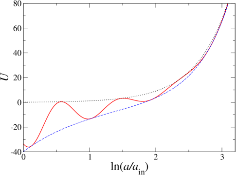
Figure 1: Effective potential for $u_{k}$ during de Sitter inflation (solid line), as a function of the number of e-folds $\ln(a/a_{\rm in})=-\ln(-H\tau)$. For comparison, the oscillation-free potential Eq. (39), and the standard de Sitter inflationary potential without coupling, $2/\tau^{2}$, are also shown (dotted line and dashed line, respectively). The parameters are $q_{\rm in}=10$ and $m/H=2\sqrt{3}$.

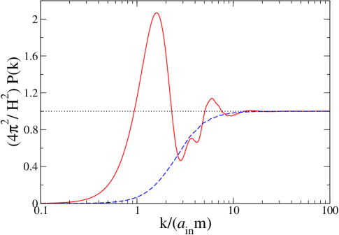
Figure 2: Power spectrum of the field $\chi$, where the evolution of $u_{k}=a\chi_{k}$ is governed by the three potentials of Fig. 1, respectively.

For the effective potential without oscillations, one observes a smooth transition between the spectrum of a very massive scalar field, which is suppressed, and the standard scale invariant spectrum of a massless scalar field. Indeed, for small $k$, i.e., large scales, the modes leave the Hubble radius when the effective mass is large, thus suppressing the power spectrum on large scales. However, as the effective mass decays with time, the amplification due to inflation becomes efficient. Since the $g^{2}\phi^{2}$ term drops down very rapidly, the transition between the strongly suppressed spectrum and the flat spectrum produced at earlier stage by inflation occurs very rapidly, within a single e-fold of inflation.

By contrast, the spectrum with an oscillating $\phi$ shows a much more complicated transition between a suppressed spectrum and the usual massless spectrum. One finds a strongly modulated spectrum with peaks and troughs. The amplitude of some peaks can be even larger than the amplitude for a massless scalar field. As we will discuss soon, this complicated spectrum is due to the combination of two opposite effects: the suppression due to a significant effective mass, the amplification due to parametric resonance.

In Fig. 3, we also show the power spectra for different values of the parameter $q_{\rm in}$, whereas Fig. 4 contains the power spectra for different values of $m/H$.

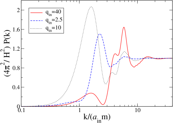
Figure 3: Spectra for various values of $q_{\rm in}=g^{2}\Phi_{\rm in}^{2}/(4m^{2})$, with ${m}/H=2\sqrt{3}$.

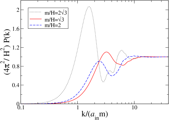
Figure 4: Spectra for various values of ${m}/H$, with $q_{\rm in}=g^{2}\Phi_{\rm in}^{2}/(4m^{2})=10$.

4.3 Discussion

In order to understand the spectra that we have computed, it is instructive to attempt an analysis similar to the preheating scenario. A key observation is that particle production occurs when the evolution is non-adiabatic, i.e., for

$$\left|{d\omega_{k}\over d\tau}\right|\ \raise 1.29167pt\hbox{$>$\kern-7.5pt\lower 4.30554pt\hbox{$\sim$}}\ \omega_{k}^{2}.$$ (40)

In the present case, there are two possible sources for the non-adiabaticity. At early times, this occurs when $\phi$ is near the origin and corresponds to a local maximum of the effective potential $U(\tau)$. At later times, for scales larger than the Hubble radius, adiabaticity is violated because of the de Sitter curvature. The first source of non-adiabaticity is the mechanism for particle production in the preheating scenario, whereas the second source is the mechanism responsible for the amplification of the vacuum fluctuations during inflation. In our case, the two effects above are combined and their relative influence on the fluctuations will be scale-dependent.

One can estimate which modes will be affected by the amplification. Substituting the effective frequency in Eq. (40) and using $\phi^{\prime}=a\dot{\phi}\simeq am\Phi_{\rm in}a^{-3/2}$ (assuming that $m\gg H$), one finds that adiabaticity is violated when

$$k^{2}\ \raise 1.29167pt\hbox{$<$\kern-7.5pt\lower 4.30554pt\hbox{$\sim$}}\ \left(a^{3/2}g^{2}\phi m\Phi_{\rm in}+\frac{2}{\tau^{3}}\right)^{2/3}-g^{2}\phi^{2}a^{2}+\frac{2}{\tau^{2}}.$$ (41)

The amplitude of the oscillations in the potential decreases exponentially with time and after a few oscillations the effect of inflation, which depends on the term $2/\tau^{2}$, dominates over the coupling to $\phi$. The moment when this happens can be estimated by requiring

$$a^{3/2}g^{2}\phi m\Phi_{\rm in}<-\frac{2}{\tau^{3}}.$$ (42)

[For $m>H$, Eq. (42) also implies that $g^{2}\phi^{2}a^{2}<2/\tau^{2}$.]

The potential $U(\tau)$, shown in Fig. 1, possesses, at early times, local maxima corresponding to the zeros of $\phi$, i.e. for $t_{j}=\frac{\pi}{m}\left(j-\frac{1}{2}\right)$, or $\tau_{j}=-H^{-1}\exp(-Ht_{j})$, for $j=1,2,\ldots$. Using Eq. (42) one sees that beyond the zero of $\phi$ labeled by $j_{\rm max}$ defined as the integer part of

$$J=\frac{1}{2}+\frac{1}{3\pi}\frac{m}{H}\ln\left[2q_{\rm in}\left(\frac{m}{H}\right)^{3}\right],$$ (43)

the de Sitter term always dominates the term due the coupling to $\phi$. During the first few $j$ oscillations, with $j<j_{\rm max}$, the main effect is the oscillating mass. Ignoring the de Sitter term, one finds that adiabaticity is violated when

$$k^{2}\ \raise 1.29167pt\hbox{$<$\kern-7.5pt\lower 4.30554pt\hbox{$\sim$}}\ a(g^{2}\phi m\Phi_{\rm in})^{2/3}-g^{2}\phi^{2}a^{2}.$$ (44)

This condition can be satisfied for small $k$ when the right hand side is positive, which implies that $\phi$ must be sufficiently close to the origin so that

$$\phi\ \raise 1.29167pt\hbox{$<$\kern-7.5pt\lower 4.30554pt\hbox{$\sim$}}\ a^{-3/4}\sqrt{m\Phi_{\rm in}/g}.$$ (45)

We have ignored here the de Sitter term. There is however a subtlety: when $\phi$ is very close to zero, then the de Sitter term necessarily dominates in the effective mass. When the condition (45) is saturated, this is the case if

$$a\ \raise 1.29167pt\hbox{$>$\kern-7.5pt\lower 4.30554pt\hbox{$\sim$}}\ \left({m\over H}\right)^{4/3}q_{\rm in}^{1/3}.$$ (46)

The de Sitter term brings a negative contribution to the effective square mass. Therefore, its effect when $\phi$ is close to zero is indeed to amplify the preheating-type effect.

From Eq. (44), during the $j$th oscillation, the maximal range of momenta where we have particle production due to the coupling to $\phi$ is then $k\leq k^{(j)}_{*}$, where

$$k^{(j)}_{*} \equiv a^{1/4}(\tau_{j})\sqrt{gm\Phi_{\rm in}}$$ (47)

$$= \sqrt{2}m\left(a(\tau_{j})q_{\rm in}\right)^{1/4},\quad{\rm for}\ \ j<j_{\rm max}.$$ (48)

In conclusion, modes with $k>k_{\rm max}$,

$$k_{\rm max}\equiv\sqrt{2}m\left(a(\tau_{j_{\rm max}})q_{\rm in}\right)^{1/4},$$ (49)

only feel the effect of inflation. We can use this equation to estimate the largest wavenumber for which we get a modulation in the spectrum and we find a very good agreement with our numerical results.

For modes with small $k$ the combined effects of, first, parametric resonance (possibly amplified by the de Sitter effect) and, later, de Sitter amplification can lead either to an enhancement or to a suppression, as illustrated by the strong modulation of the spectra on large scales. The effects are subtle. For example, increasing the value of $q_{\rm in}$ tends to make the parametric resonance more efficient but at the same time, a large $q_{\rm in}$ implies that the effective mass will be on average larger and can thus lead to a suppression of the power spectrum generated by inflation.

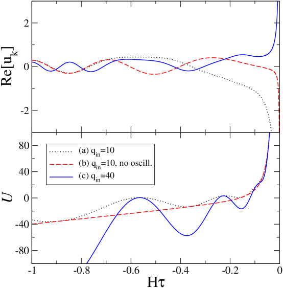
Figure 5: Upper panel: evolution of the mode $k=1$ in three cases; (a): $q_{\rm in}=10$; (b): $q_{\rm in}=10$, with the oscillation-free potential of Eq. (39), and (c): $q_{\rm in}=40$. Lower panel: the effective potential for the three cases.

To illustrate how the various effects can combine, we have plotted in Fig. 5 the time evolution of the mode $k=1$ in three different cases: (a): $q_{\rm in}=10$; (b): $q_{\rm in}=10$, but with the oscillation-free potential given in Eq. (39), and (c): $q_{\rm in}=40$. In parallel, we have plotted the effective potential $U(\tau)$ for the three cases. From the spectra plotted in Fig. 2 and Fig. 3 we know that the case (a) corresponds to a strong enhancement while the case (c) is strongly suppressed and (b) even more. The time evolution is instructive: the case (b) oscillates regularly and is strongly amplified at late times by the de Sitter effect, although it has not been amplified by the parametric resonance before. In the cases (a) and (c), the effect of the oscillating mass is clearly visible. When the effective mass approaches zero, near $H\tau=-0.6$, the oscillation of the modes is suspended and their amplitude slightly increases. One also sees why the case (c) corresponds to a strong suppression. This is because the effective mass, still important near $H\tau=-0.23$, exerts a restoring force which reduces the amplitude before the final increase due to the de Sitter amplification.

5 Power-law inflation

So far, we have assumed that the inflationary phase was described by a pure de Sitter phase, characterized by a constant $H$. This implies that the scalar field has always been oscillating in the past and we were obliged to start the computation, somewhat artificially, at a local extremum of $\phi$. More realistically, the Hubble parameter is expected to decrease during inflation. This significantly changes the past of the scenario since the massive scalar field $\phi$ is frozen during the early stage of inflation when $H\gg m_{\phi}$. Later, when the Hubble parameter becomes smaller than its mass, $\phi$ starts to oscillate.

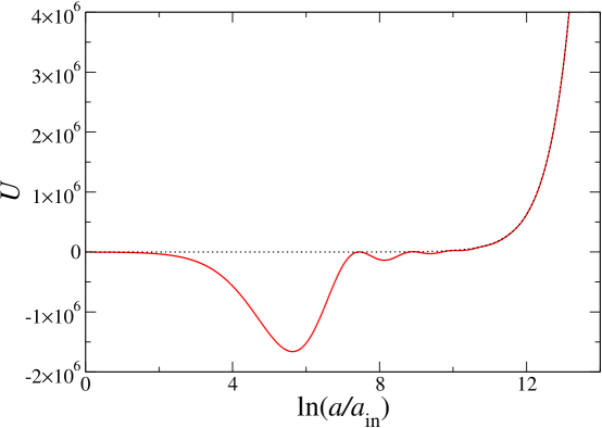
Figure 6: Potential $U$ for power law-inflation, with $p=5$, where $a\propto t^{p}$. For this example we have used $q_{\rm in}=6.25\times 10^{5}$.

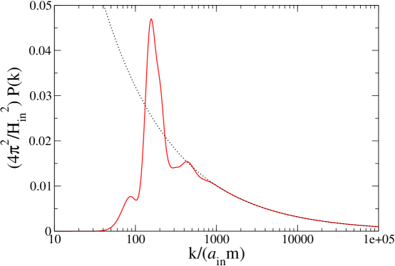
Figure 7: Power spectrum of the field $\chi$ corresponding to the effective potential $U$ of Fig. 6.

In order to implement this more realistic scenario, one can assume that the universe undergoes a power-law inflation [9], so that the scale factor evolves like

$$a(t)\propto t^{p},\qquad p\gg 1.$$ (50)

Then the equation of motion for $\phi$ reads

$$\ddot{\phi}+{3p\over t}\dot{\phi}+m_{\phi}^{2}\phi=0,$$ (51)

and the solution of this equation that does not diverge when $t\rightarrow 0$ is given by

$$\phi=\phi_{0}\Gamma(\nu+1)\left({m_{\phi}\,t\over 2}\right)^{-\nu}J_{\nu}(m_{\phi}\,t),\quad\nu=(3p-1)/2,$$ (52)

where $\phi_{0}$ is the asymptotic value of $\phi$ when $t\rightarrow 0$ and $J_{\nu}$ is the Bessel function of order $\nu$. As long as $m_{\phi}\,t\ll 1$, $\phi$ remains frozen at the value $\phi_{0}$. When $t$ is of the order of $m_{\phi}^{-1}$, the scalar field starts to evolve and subsequently oscillates while its amplitude decreases like $a^{-3/2}$.

We have plotted in Fig. 6 the effective potential corresponding to this scenario and one sees indeed that in the asymptotic past $U(\tau)$ goes to zero, in contrast with the de Sitter case of the previous section. We have also computed the power spectrum associated with this effective potential in Fig. 7. We observe the same features as in the de Sitter case: a transition from a suppressed spectrum to a standard massless spectrum, which is not scale-invariant here since we are in power-law inflation (the massless spectrum is shown as a dotted line), with a strong modulation.

In order to relate the present scenario with that of the previous section, it is useful to evaluate the amplitude of the scalar field $\phi$ deep in the oscillatory regime where (23) is a good approximation as a function of its initially frozen amplitude $\phi_{0}$. Using the asymptotic behavior $J_{\nu}(z)\simeq\sqrt{2/(\pi z)}\cos(z-\pi(2\nu+1)/4)$ for $z\gg 1$, one can evaluate the amplitude of the scalar field at time $t\gg m_{\phi}^{-1}$. One finds

$$\Phi(t)\sim\phi_{0}2^{-\nu}\Gamma(\nu+1)\left({m_{\phi}p\over H}\right)^{-3p/2},$$ (53)

where we have used $t=p/H$. This gives roughly

$$\Phi(t)\sim\phi_{0}\left({3H\over 4m_{\phi}e}\right)^{3p/2}.$$ (54)

Since $3H/(2m_{\phi})<1$, one sees that the ratio $\Phi/\phi_{0}$ becomes extremely small for large values of $p$.

6 Observational consequences

The purpose of this section is to discuss whether the phenomena studied in the present work could be of any relevance from an observational point of view, in particular in the CMB fluctuations. This is reminiscent of the question whether preheating could significantly affect super-Hubble perturbations [10].

Let us first stress that, since $\chi$ is not the inflaton in our model, its spectrum will not be directly relevant if the CMB fluctuations observed today are essentially due to the inflaton fluctuations. However, this is not necessarily the case as demonstrated recently by the curvaton [3, 4, 5] and inhomogeneous reheating scenarios [11, 12, 13], in which the primordial perturbations are generated by a light field that is not driving inflation.

Could, then, our field $\chi$ be a curvaton? If one starts from the potential given in Eq. (18), it does not seem to be a viable idea. Indeed, as mentioned earlier, the background value of $\chi$ has been driven to zero by its initially large effective mass and, even after $\phi$ has fallen to zero, there is a priori no reason for $\chi$ to acquire a non-zero expectation value. This is problematic because the energy density fluctuations due to the scalar field $\chi$ will be, instead of linear, quadratic in $\delta\chi$ and will not have the required Gaussian properties [3].

This objection, however, can be evaded by a slight modification of the scalar field potential, which does not change the power spectrum generated during inflation. Let us consider a potential of the form

$$V(\phi,\chi)={\textstyle{1\over 2}}m_{\phi}^{2}\phi^{2}+{\textstyle{1\over 2}}g^{2}\phi^{2}\left(\chi-\chi_{0}\right)^{2}+{\textstyle{1\over 2}}m_{\chi}^{2}\chi^{2},$$ (55)

where $m_{\chi}$ is a mass scale much smaller than the Hubble parameter during inflation, as required for a curvaton. The above potential has different minima for $\chi$, depending on the value of $\phi$. In the very early universe, when the value of $\phi$ is big, $\chi$ is driven towards the value $\chi_{0}$ because of the second term in the potential. The field $\phi$ subsequently oscillates towards zero. However, because of the Hubble friction, the scalar field $\chi$ remains frozen at its fixed value $\chi_{0}$ for a while. Eventually, when $H$ reaches down the value $m_{\chi}$, $\chi$ starts oscillating about its low-energy minimum $\chi=0$, as a standard curvaton. If $\chi$ oscillates for long enough before decaying, it will eventually dominate the energy density of the universe, because its energy density decreases more slowly that the radiation produced by the inflaton decay. This implies that the isocurvature $\chi$ fluctuations are converted into curvature perturbations [3],

$$\zeta=\frac{2}{3}\frac{\delta\chi_{*}}{\chi_{*}},$$ (56)

where, $\zeta\equiv-H\delta\rho/\dot{\rho}$ is the uniform energy density perturbation, here written in the spatially flat gauge. The star refers to the expectation value of $\chi$ during inflation, and thus $\chi_{*}=\chi_{0}$, and $\delta\chi_{*}$ corresponds to the fluctuations generated during inflation.

In this context, one sees that $\chi$ behaves exactly as a curvaton, with the only exception that its quantum fluctuations during inflation are affected by the evolution of the scalar field $\phi$. Therefore, if the usual conditions for neglecting the inflaton perturbations with respect to the curvaton perturbations are satisfied, then the CMB fluctuations would contain the special features discussed in the previous sections. One could also envisage the possibility that the primordial spectrum is the combination of a standard inflaton spectrum and of a modulated spectrum of the kind discussed here [14].

One legitimate question is then whether the peculiar features of our modulated spectra could account for the “anomalies” that seem to be suggested by the WMAP data [15, 16]: the so-called cosmic variance outliers (points which lie outside the one sigma cosmic variance) are present either on large scales, in the suppression of the lower multipoles, and on smaller scales, where the power spectrum seems to contain features in the form of spikes or waves. Several works (see e.g. [18, 17, 19, 20] for the lowest multipoles and [21, 22] for higher multipoles) have suggested various modifications of the early universe scenario to account for this.

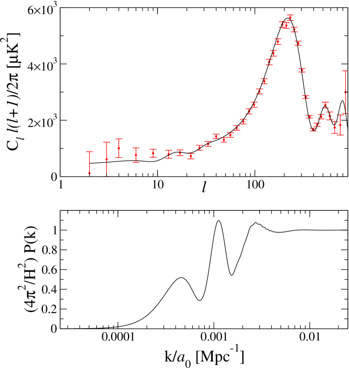
Figure 8: In the upper panel, an example of spectrum of CMB anisotropies generated by a primordial curvaton power spectrum with modulated fluctuations, computed by modifying CAMB [23]. We use the minimal set of $\Lambda$CDM model parameters from the best fit to the WMAP data alone as provided by [16]. No running of the spectral index or tensor contribution have been included. The latter would rise the CMB spectrum on large scales helping to fit the data. The spectrum is compared to the first year WMAP data. In the lower panel the corresponding power spectrum of $\chi$, generated by using the parameters $q_{\rm in}=40$ and $m/H=2\sqrt{2}$.

It is not the purpose of the present work to investigate systematically this question. We will just limit ourselves to a few remarks. The power spectrum of $\chi$ as derived in Sec. 4 has two characteristics: a strong suppression on very large scales and a series of few oscillations on slightly smaller scales. On smaller length-scales, for $k\ \raise 1.29167pt\hbox{$>$\kern-7.5pt\lower 4.30554pt\hbox{$\sim$}}\ k_{\rm max}$, it is featureless and close to scale invariant. In [18] it was noticed that the WMAP data are consistent with a primordial power spectrum which is featureless for the modes $k/a_{0}\ \raise 1.29167pt\hbox{$>$\kern-7.5pt\lower 4.30554pt\hbox{$\sim$}}\ 0.005\ {\rm Mpc}^{-1}$. Thus the modulations should affect modes with larger length-scales.

As an illustration, we have constructed such an example of modulated power spectrum, shown in the lower panel of Fig. 8, with the parameters $q_{\rm in}=40$ and $m/H=2\sqrt{2}$. In the upper panel, we have plotted the corresponding spectrum for CMB anisotropies, computed by modifying CAMB [23]. The large scale plateau of the CMB anisotropies is suppressed for $\ell\ \raise 1.29167pt\hbox{$<$\kern-7.5pt\lower 4.30554pt\hbox{$\sim$}}\ 30$, corresponding to the suppression of the power spectrum of $\chi$, on very large scales, $k/(a_{0}{\rm Mpc}^{-1})\ \raise 1.29167pt\hbox{$<$\kern-7.5pt\lower 4.30554pt\hbox{$\sim$}}\ 10^{-3}$. Furthermore, the oscillations in the $\chi$ spectrum for the intermediate scales translate into oscillations in the CMB spectrum for $10\ \raise 1.29167pt\hbox{$<$\kern-7.5pt\lower 4.30554pt\hbox{$\sim$}}\ \ell\ \raise 1.29167pt\hbox{$<$\kern-7.5pt\lower 4.30554pt\hbox{$\sim$}}\ 40$.

Note however that in order for these features to be observable, the modulations due to the oscillating mass must affect, during inflation, precisely the scales that have reentered the Hubble radius recently, i.e. the scales corresponding to the largest observable scales. A similar problem hampers the models trying to explain particular features with a modification of the early universe dynamics.

7 Conclusions

In the present work, we have investigated the amplification of the quantum fluctuations of a test scalar field $\chi$ during inflation, when this scalar field has an oscillating effective mass, resulting from its coupling to a massive scalar field $\phi$ that oscillates during inflation.

We have computed numerically the final power spectrum for the fluctuations, which in the context of de Sitter inflation, depends only on two parameters: the ratio $m_{\phi}/H$ and the (initial) coupling parameter $q_{\rm in}=g^{2}\Phi_{\rm in}^{2}/(4m^{2})$. The power spectrum is characterized by a transition from a suppressed spectrum on large length-scales to a standard massless spectrum on smaller length-scales. On the intermediate scales, the spectrum can be affected by strong modulations.

Our scenario shares with the preheating scenario the essential ingredient of an effective oscillating mass. However, in our case, the universe is accelerating whereas, in the preheating scenario, taking place after inflation, the universe is decelerating. As a consequence, instead of particle production in the usual sense, the fluctuations, in our case, are amplified on super-Hubble scales. Moreover, in addition to the parametric resonance due the oscillating mass, our scenario is also characterized by an amplification due to the acceleration of the background cosmology.

We have also discussed a possible observational signature of our scenario when the scalar field $\chi$ is assumed to be a curvaton field. We have shown that the corresponding CMB multipole spectrum is characterized by a suppression on large angular scales and a modulation on slighter smaller scales, with respect to the standard power spectrum.

Acknowledgements We wish to thank Justin Khoury for stimulating discussions and instructive comments. F.V. acknowledges financial support from the Swiss National Science Foundation.

References

- [1] A. Linde, Particle physics and inflationary cosmology (Harwood Academic Publisher, Chur, Switzerland 1990); A. R. Liddle and D. H. Lyth, Cosmological inflation and large scale structure (Cambridge University Press, Cambridge, 2000)
- [2] V. F. Mukhanov, H. A. Feldman, R. H. Brandenberger, Phys. Rep. 215, 203-333 (1992).
- [3] D. H. Lyth, D. Wands, Phys. Lett. B 524, 5-14 (2002).
- [4] K. Enqvist and M. S. Sloth, Nucl. Phys. B 626, 395 (2002).
- [5] T. Moroi and T. Takahashi, Phys. Lett. B 522, 215 (2001) [Erratum-ibid. B 539, 303 (2002)].
- [6] L. Kofman, A. D. Linde and A. A. Starobinsky, Phys. Rev. D 56, 3258 (1997).
- [7] C. P. Burgess, J. M. Cline, F. Lemieux and R. Holman, JHEP 0302, 048 (2003).
- [8] M. Abramowitz and I. A. Stegun, Handbook of mathematical functions (Dover publications, INC., New York, 1964).
- [9] F. Lucchin and S. Matarrese, Phys. Lett. B164, 282 (1985).
- [10] B. A. Bassett, F. Tamburini, D. I. Kaiser, and R. Maartens, Nucl. Phys. B561, 188 (1999); B. A. Bassett, D. I. Kaiser, and R. Maartens, Phys. Lett. B 455, 84 (1999); F. Finelli and R. Brandenberger, Phys. Rev. Lett. 82, 1362 (1999); ibid., Phys. Rev. D 62, 083502 (2000); K. Jedamzik and G. Sigl, Phys. Rev. D 61, 023519 (2000); C. Gordon, D. Wands, B. A. Bassett and R. Maartens, Phys. Rev. D 63, 023506 (2001).
- [11] G. Dvali, A. Gruzinov and M. Zaldarriaga, Phys. Rev. D 69, 023505 (2004).
- [12] L. Kofman, [arXiv:astro-ph/0303614].
- [13] F. Vernizzi, Phys. Rev. D 69, 083526 (2004).
- [14] D. Langlois and F. Vernizzi, Phys. Rev. D 70, 063522 (2004).
- [15] C. L. Bennet et al., Astrophys. J. Suppl. 148, 1 (2003).
- [16] D. N. Spergel et al., Astrophys. J. Suppl. 148, 175 (2003).
- [17] H. V. Peiris et al., Astrophys. J. Suppl. 148, 213 (2003).
- [18] S. L. Bridle, A. M. Lewis, J. Weller, and G. Efstathiou, Mon. Not. R. Astron. Soc. 342, L72 (2003).
- [19] C. Contaldi, M. Peloso, L. Kofman, A. Linde, JCAP 0307, 002 (2003).
- [20] J. M. Cline, P. Crotty, J. Lesgourgues, JCAP 0309, 010 (2003).
- [21] J. Martin and C. Ringeval, Phys. Rev. D 69, 083515 (2004); ibid. Phys. Rev. D 69, 127303 (2004); ibid. J. Martin and C. Ringeval, [arXiv:hep-ph/0405249].
- [22] P. Hunt and S. Sarkar, [arXiv:astro-ph/0408138].
- [23] A. Lewis, A. Challinor, A. Lasenby, Astrophys. J. 538, 473 (2000); A. Lewis, and S. Bridle, Phys. Rev. D 66, 103511 (2002); http://camb.info.