Non-stationary variability in AGN: the case of 3C 390.3

We use data from a two-year intensive RXTE monitoring campaign of the broad-line radio galaxy 3C~390.3 to investigate its stationarity. In order to exploit the potential information contained in a time series more efficiently, we use a multi-technique approach. Specifically, the temporal properties are first studied with a non-linear technique borrowed from non-linear dynamics. Then we utilize traditional linear techniques both in the Fourier domain, by estimating the power spectral density, and in the time domain with a structure function analysis. Finally we investigate directly the probability density function associated with the physical process underlying the signal. All the methods demonstrate the presence of non-stationarity. The structure function analysis, and (at a somewhat lower significance level) the power spectral density suggest that 3C 390.3 is not even second order stationarity. This result indicates, for the first time, that the variability properties of the active galactic nuclei light curves may also vary with time, in the same way as they do in Galactic black holes, strengthening the analogy between the X-ray variability properties of the two types of object.

1 Introduction

Among the basic properties characterizing an Active Galactic Nucleus (AGN) the flux variability, especially at X-rays, is one of the most common. Previous multi-wavelength variability studies (e.g., Edelson et al. 1996; Nandra et al. 1998) have shown that AGN are variable in every observable wave band, but the X-ray flux exhibits variability of larger amplitude and on time scales shorter than any other energy band, indicating that the X-ray emission originates in the innermost regions of the central engine.

However, even though the discovery of X-ray variability dates back more than two decades, its origin is still poorly understood. Nevertheless, it is widely acknowledged that the variability properties of AGN are an important means of probing the physical conditions in their emission regions. The reason is that using energy spectra alone it is often impossible to discriminate between competing physical models and thus the complementary information obtained from the temporal analysis is crucial to break the spectral degeneracy.

Over the years, several variability models have been proposed, involving one or a combination of the fundamental components of an AGN: accretion disk, corona, and relativistic jet. These models can be divided into two main categories: 1) intrinsically linear models, as the shot noise model (e.g., Terrel 1972), where the light curve is the result of the superposition of similar shots or flares produced by many independent active regions, and 2) non-linear models, which require some coupling between emitting regions triggering avalanche effects, as the self-organized criticality model (e.g., Mineshige et al.1994), or models assuming that the variability is caused by variations in the accretion rate propagating inwards (e.g. Lyubarskii 1997). The “rms-flux relation” recently discovered by Uttley & McHardy (2001), along with detection of non-linearity in different AGN light curves (i.e., in 3C 345 by Vio et al. 1992; in 3C 390.3 by Leighly & O’Brien 1997; in NGC 4051 by Green et al. 1999; in Ark 564 by Gliozzi et al. 2002), favors non-linear variability models, but there is no general consensus on the nature of the X-ray variability yet.

Because of their brightness, the temporal and spectral properties of Galactic black holes (GBHs) are much better known and can be used to infer information on their more powerful, extragalactic analogues, the AGN. For example, it is well established that GBHs undergo state transitions (see McClintock & Remillard 2003 for a recent review), switching between “low” and “high” states, which are both unambiguously characterized by a specific combination of energy spectrum and power spectral density (PSD).

Early AGN PSD studies based on EXOSAT data (e.g., Lawrence & Papadakis 1993; Green et al. 1993) revealed a red-noise variability (i.e., a PSD described by a power law), similar to the one observed in GBHs, which in addition show breaks in their PSD (i.e., departure from the power law) at specific frequencies depending on the spectral state. Recently, power-spectral analysis of high-quality light curves of a few AGN (obtained with RXTE and XMM-Newton  e.g., Uttley, et al. 2002; Markowitz et al. 2003; McHardy et al. 2004) has led to the first unambiguous detection of “frequency breaks” in their power spectra, strengthening the similarity between the AGN and GBH PSDs. This similarity lends further support to the hypothesis that the same physical process is at work in AGN and GBHs, regardless of the black hole mass.

Almost all methods employed in timing analysis (e.g., power spectrum, structure function, auto-correlation analysis) require some kind of stationarity. Generally speaking, a system is considered stationary, if the average statistical properties of the time series are constant with time. More specifically, the stationarity is defined as “strong” if all the moments of the probability distribution function are constant, and “weak” if only the moments up to the second order (i.e., mean and variance) are constant. Usually, non-stationarity is considered an undesired complication. However, in some cases the non-stationarity provides the most interesting information, as in the case of GBHs switching from a spectral state to another.

Figure 1: X-ray light curves of the background-subtracted count rate in the 2–20 keV band (top panel) and of the X-ray color 7–20 keV/2–5 keV (bottom panel) from RXTE PCA observations of 3C 390.3. Time bins are 5760s ($\sim$ 1 RXTE orbit). Filled circles represent data points from the first monitoring campaign from 1999 January 8 to 2000 February 29, whereas open diamonds are data points from the second monitoring campaign from 2000 March 3 to 2001 February 23. The dashed lines in the top panel indicate the intervals used for the time-resolved spectral analysis (see $\S$9).

Compared to their scaled-down counterparts, the GBHs, the study of non-stationarity in AGN is complicated by the fact that their flux variability is characterized by much longer time-scales. This might be the reason why “different” states have not been observed yet in AGN, even though a correspondence between GBH spectral states and some AGN classes (namely, between Seyfert 1 galaxies and the GBH low state, and between Narrow-Line Seyfert 1 galaxies and the GBH high state, respectively) has been hypothesized. Nonetheless, several monitoring campaigns carried out by RXTE in the last decade have produced archival data sets suitable for searching for non-stationarity in the AGN light curves. Such a detection of non-stationarity would suggest transitions of the source between different states.

We use data from a two-year intensive RXTE monitoring campaign of the broad-line radio galaxy (BLRG) 3C~390.3 to search for evidence of non-stationarity. Previous X-rays studies with ROSAT, and RXTE (Leighly & O’Brien 1997, Gliozzi et al. 2003) demonstrated that 3C 390.3 is one of the most variable AGN on time scales of days and months. In addition, the ROSAT HRI monitoring campaign has shown evidence for non-linearity and possibly non-stationarity (Leighly & O’Brien 1997). In order to exploit all the information contained in the time series, we employ a number of complementary methods. Specifically, we investigate the stationarity in 3C~390.3 not only with traditional linear techniques as the PSD in the Fourier domain, and the structure function (SF) and auto-correlation function (ACF) in the time domain, but also in pseudo-phase space, with techniques borrowed from nonlinear dynamics, and finally we probe directly the probability density function (PDF) associated with the physical processes underlying the signal.

2 Observations and Data Reduction

We use archival RXTE data (PI: Leighly) of 3C 390.3. This source was observed by RXTE for two consecutive monitoring campaigns between 1999 and 2001. The first set of observations was carried out from 1999 January 8 to 2000 February 29, and the second one from 2000 March 3 to 2001 February 23. Both campaigns were performed with similar sampling: 3C 390.3 was regularly observed for $\sim$ 1000–2000 s once every three days. The observations were carried out with the Proportional Counter Array (PCA; Jahoda et al. 1996), and the High-Energy X-Ray Timing Experiment (HEXTE; Rotschild et al. 1998) on RXTE. Here we will consider only PCA data, because the signal-to-noise of the HEXTE data is too low for a meaningful timing analysis.

The PCA data were screened according to the following acceptance criteria: the satellite was out of the South Atlantic Anomaly (SAA) for at least 30 minutes, the Earth elevation angle was $\geq 10^{\circ}$, the offset from the nominal optical position was $\leq 0^{\circ}\!\!.02$, and the parameter ELECTRON-0 was $\leq 0.1$. The last criterion removes data with high particle background rates in the Proportional Counter Units (PCUs). The PCA background spectra and light curves were determined using the ${\rm L}7-240$ model developed at the RXTE Guest Observer Facility (GOF) and implemented by the program pcabackest v.2.1b. Since the two monitoring campaigns span three different gain epochs, the appropriate files provided by the RXTE Guest Observer Facility (GOF), were used to calculate the background light curves. This model is appropriate for “faint” sources, i.e., those producing count rates less than 40 ${\rm s^{-1}\leavevmode\nobreak\ PCU^{-1}}$. All the above tasks were carried out using the FTOOLS v.5.1 software package and with the help of the rex script provided by the RXTE GOF, which also produces response matrices and effective area curves appropriate for the time of the observation. Data were initially extracted with 16 s time resolution and subsequently re-binned at different bin widths depending on the application. The current temporal analysis is restricted to PCA, STANDARD-2 mode, 2–20 keV, Layer 1 data, because that is where the PCA is best calibrated and most sensitive. Since PCUs 1, 3, and 4 were frequently turned off (the average number of PCUs is 2.25 and 1.95 in the 1999 and 2000 observations, respectively), only data from the other two PCUs (0 and 2) were used. All quoted count rates are for two PCUs.

The spectral analysis of PCA data was performed using the XSPEC v.11 software package (Arnaud 1996). We used PCA response matrices and effective area curves created specifically for the individual observations by the program pcarsp, taking into account the evolution of the detector properties. All the spectra were rebinned so that each bin contained enough counts for the $\chi^{2}$ statistic to be valid. Fits were performed in the energy range 4–20 keV, where the signal-to-noise ratio is the highest.

3 The X-ray Light Curve

Figure 1 shows the background-subtracted 2–20 keV count rate and hardness ratio (7–20 keV/2–5 keV) light curves of 3C 390.3. Filled circles represent data points from the first monitoring campaign, whereas open diamonds are used for the second campaign. A visual inspection of the light curve suggests the existence of different variability patterns during the two monitoring campaigns. In the first one, 3C 390.3 exhibits an initial smooth decrease in the count rate (a factor $\sim$2 in 100 days) followed by an almost steady increase (a factor $\sim$3.5 in 100 days). After day $\sim$ 200 (from the beginning of the observation), the source shows significant, low-amplitude, fast variations. During the second monitoring campaign, the source does not show any long-term, smooth change in count rate, but only a flickering behavior with two prominent flares. This qualitative difference is supported by the difference of the two mean count rates averaged over each campaign, $6.4\pm 0.2{\leavevmode\nobreak\ \rm s^{-1}}$ and $9.0\pm 0.1{\leavevmode\nobreak\ \rm s^{-1}}$ respectively, where the uncertainties, $\sigma/\sqrt{n}$, were calculated assuming that the data distribution is normal and the data are a collection of independent measurements. However, the data points of AGN light curves are not independent but correlated and thus the apparent difference between the mean count rates could simply result from the red-noise nature of the variability process, combined with its randomness.

Any AGN light curve is just one of the possible realizations of an underlying physical process, which can be linear stochastic, non-linear stochastic, chaotic, or a combination of the three possibilities. The distinction between stochastic and chaotic processes is that the former are random, whereas the latter are deterministic. A further difference is that chaotic processes are intrinsically non-linear, while stochastic processes can be either linear or non-linear (in a mathematical sense linearity means that the value of the time series at a given time can be written as a linear combination of the values at previous times plus some random variable). As a consequence, light curves produced by the same process may appear different, but the average statistical properties should in principle be constant, provided that the system is actually stationary, and the light curves are longer than the characteristic time scale of the system. This indicates that only average statistical properties can provide information on the physics underlying a variability process, whereas instantaneous properties (such as the visual appearance of the light curves) may be misleading. With this in mind, we carry out a number of tests for stationarity, which we describe in detail in the next section.

4 Stationarity Tests

In previous temporal studies of AGN, no strong evidence for non-stationarity has been reported. Indeed, AGN light curves are considered to be “second-order” stationary, due to their red noise variability. However, the absence of non-stationarity might be partly due to the fact that previous works were based only on a PSD analysis, which may not be the most appropriate method to detect non-stationarity in some cases, as we demonstrate below.

Here, we adopt several complementary methods to investigate the issue of the stationarity in the 3C~390.3 light curve. First, we utilize the scaling index method, a technique borrowed from non-linear dynamics, useful for discriminating between time series. Secondly, the temporal properties are studied first with traditional linear techniques in the Fourier domain, by estimating the PSD, and in the time domain with structure function and auto-correlation function analyses. Finally, we probe directly the probability density function associated with the physical process underlying the signal. We demonstrate that all methods, with the exception of the PSD, point very strongly to non-stationarity.

4.1 Non-linear Analysis: Scaling Index Method

Non-linear methods are rarely employed in the analysis of AGN light curves, partly because these methods are less developed than the linear ones, partly because it is implicitly assumed that AGN light curves are linear and stochastic. However, non-linear methods can be useful not only to characterize the nature of chaotic deterministic systems, but also to discriminate between two time series, regardless of the fact that they are linear or non-linear.

The scaling index method (e.g., Atmanspacher et al. 1989) is employed in a number of different fields because of its ability to discern underlying structure in noisy data. It was applied to AGN time series by Gliozzi et al. (2002) to show that the low and high states of the Narrow-Line Seyfert 1 galaxy Ark~564, indistinguishable on the basis of linear methods, are actually intrinsically different. A detailed description of the method is given in Gliozzi et al. (2002) and references therein; here we summarize its basic characteristics.

When methods of nonlinear dynamics are applied to time series analysis, the concept of phase space reconstruction represents the basis for most of the analysis tools. In fact, for studying chaotic deterministic systems it is important to establish a vector space (the phase space) such that specifying a point in this space specifies a state of the system, and vice versa. However, in order to apply the concept of phase space to a time series, which is a scalar sequence of measurements, one has to convert it into a set of state vectors.

For example, starting from a time series, one can construct a set of 2(3, 4, …)-dimensional vectors by selecting pairs (triplets, quadruplets, …) of data points, whose count rate values represent the values of the different components of each vector. The data points defining the vector components are chosen such that the second point is separated from the first by a time delay $\Delta t$, while the second is separated from the first by $2\Delta t$, and so on. This process, called time-delay reconstruction, can be easily generalized to any n-dimensional vector. In non-linear dynamics, where this technique is used to determine fractal dimensions and discriminate chaos from stochasticity, the choice of the time delay is not arbitrary, but should satisfy specific rules (see Kantz & Schreiber 1997 for a review). In our case, however, this technique is used only to discriminate between two states of the system (determining any kind of dimension would be meaningless for non-deterministic systems). Thus the only requirement here is that the results are statistically significant. Nonetheless, we have used different values for $\Delta t$, and verified that the results do not critically depend upon the choice of the time delay.

The set of n-dimensional vectors, derived from the original light curve, are then mapped (or embedded) into an n-dimensional vector space, producing a phase space portrait, whose topological properties represent the temporal properties of the corresponding time series.

In order to quantify the difference between two phase space portraits, a suitable quantity is the correlation integral $C(R)$ (Grassberger & Procaccia 1983), which basically counts the number of pairs of points with distances smaller than $R$. An exhaustive description of the correlation integral method and its application to X–ray light curves of AGN is given by Lehto et al (1993).

Figure 2: Scaling index distributions of 3C~390.3 during the 1999 (dashed line) and 2000 (solid line) monitoring campaign.

The scaling index method, which is based on the local estimate of the correlation integral for each point in the phase space, characterizes quantitatively the data point distribution by estimating the “crowding” of the data around each data point. More specifically, for each of the N points, the cumulative number function is calculated

$$N_{i}(R)=n\{j|d_{ij}\leq R\},$$ (1)

In other words, $N_{i}(R)$ measures the number of points $j$, whose distance $d_{ij}$ from a point $i$ is smaller than $R$. The function $N_{i}(R)$, in a given range of radii (which are related to the typical distances between the data points, that, in turn, depend on the choice of the embedding space dimension), can be approximated by a power law $N_{i}(R)\sim R^{\alpha_{i}}$, where $\alpha_{i}$ is the scaling index. Explicitly, the scaling index for each point $i$ is obtained by calculating the cumulative number function $N_{i}(R)$ at two different radii, $R_{1}$ and $R_{2}$, and by computing the logarithmic slope:

$${\alpha_{i}}=\frac{\log N_{i}(R_{1})-\log N_{i}(R_{2})}{(\log R_{1}-\log R_{2})}.$$ (2)

Note that for a purely random process the average scaling index $\langle\alpha\rangle$ tends to the value of the dimension of the embedding space, whereas for correlated processes and for deterministic (chaotic) processes the value of $\langle\alpha\rangle$ is always smaller than the dimension of the embedding space and independent of that dimension.

We have calculated the scaling index for all the points of the two phase space portraits derived from the two monitoring campaigns, using embedding spaces of dimensions ranging between 3 and 10. There are no systematic prescriptions for the choice of the embedding dimension. The discriminating power of the statistic based on the scaling index is enhanced using high embedding dimensions (this can be understood in the following way: if the data are embedded in a low-dimension phase-space many of them will fall on the same position, losing in this way part of the information). On the other hand, the choice of too high embedding dimensions would reduce the number of points in the pseudo phase-space, lowering the statistical significance of the test. In all cases a significant difference from the two light curves was found. The resulting histograms for a 5-dimensional phase space are plotted in Fig 2: the dashed line represents data from the first monitoring campaign, whereas the continuous line indicates points from the second monitoring campaign.

There is a remarkable difference between the two distributions, both in shape and location of the centroid. For this kind of analysis the most important quantity is the location of the centroid of the histogram, which is related to the correlation dimension. Such a difference cannot be ascribed to the difference in mean count rates showed during the two monitoring campaigns. In fact, the scaling index analysis is sensitive only to the relative positions of the data points within a distribution, not to their absolute positions in the phase space. This has been verified applying the scaling index analysis to randomized light curves, which were obtained by randomizing the temporal positions of the data points of each light curve. In this way, the statistical properties (i.e., the mean, variance, and the statistical moments of higher order) of the light curves are unchanged, whereas the timing structure is destroyed. As expected, the centroids of the histograms of the randomized distributions have larger values and are nearly indistinguishable.

We conclude that, the intrinsic, timing properties of the 1999 light curve are significantly different from the properties of the 2000 light curve. This result suggests that the X-ray emitting process in 3C 390.3 is non stationary.

4.2 Analysis in the Fourier Domain: Power Spectral Density

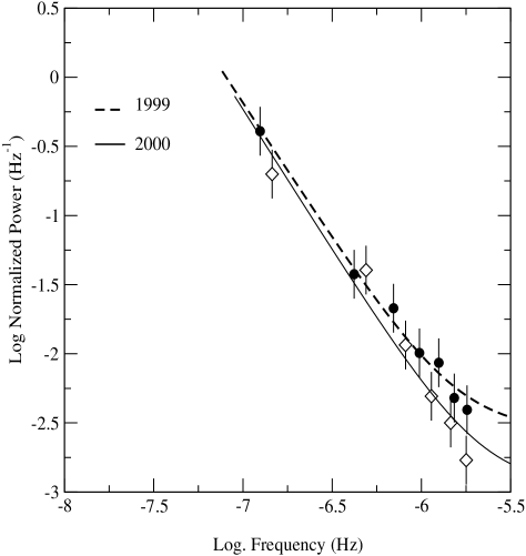
Figure 3: RXTE PCA power density spectra using based on the 1999 and 2000 light curves with 3-day bins, normalized to their mean (filled circles and open diamonds, respectively). The solid and dashed lines show the best fitting power law models, including the effects of the experimental Poisson noise level.

We followed the method of Papadakis & Lawrence (1993) to compute the power spectrum of the 1999 and 2000 light curves, after normalizing them to their mean. We used a 3-day binning (i.e., equal to the typical sampling rate of the source) for both light curves. As a result, the light curves that we used are evenly sampled, but there are a few missing points in them; 30 out of 140 and 15 out of 120 for the 1999 and 2000 light curves, respectively. These points are randomly distributed over the whole light curve, and we accounted for them using linear interpolation between the two bins adjacent to the gaps, adding appropriate Poisson noise.

Figure 3 shows the PSD of the 1999 and 2000 light curves (filled circles, and open diamonds, respectively). Each point in the estimated PSD represents the average of 10 logarithmic periodogram estimates. Both PSDs follow a power-law like form, with no obvious frequency breaks. We fitted both spectra with a simple power law. The model provides a good description of both PSDs. The best fitting slope values are consistent within the errors with the value of $-2\pm 0.3$ in both cases. The best fitting power law models are also shown in Fig 3 (solid and dashed lines, for the 2000 and 1999 PSDs, respectively).

A closer look at the PSD plot (Fig. 3) indicates a possible low frequency flattening of the 2000 PSD between $\log(\nu)=-6.5$ and $-7$, corresponding to a time interval between $\sim$35 and 115 days. In order to investigate this issue further we split the two lowest frequency points into two (to increase the frequency resolution) and refitted the 2000 PSD with a broken power law model. We kept the slope below and above the frequency break fixed to the values $-1$ and $-2$, respectively, and kept as free parameters the break frequency and normalization of the PSD. The model provides a good fit to the 2000 PSD, but statistically not better than a simple power law according to an F-test. The best fitting break frequency is $2.5\times 10^{-7}$ Hz, which corresponds to a break time scale of $\sim 46$ days. The $90\%$-confidence lower limit to this time scale is 33 days, while, due to the limited coverage of the observed PSD at lower frequencies, the upper limit is effectively equal to the length of the 2000 light curve (i.e. $\sim 300$ days). We also tried to fit the 1999 PSD with this model, but without success: the best fitting break frequency turned out to be lower than the lowest frequency sampled by the 1999 light curve, indicating that there is no indication of any breaks in the 1999 PSD. This power spectrum follows a $-2$ power law shape down to the lowest sampled frequencies.

In order to quantify the comparison between the 1999 and 2000 PSDs in a statistical way, we used the “S” statistic as defined by Papadakis & Lawrence (1995). To avoid the constant Poisson noise level, we considered the periodogram estimates up to frequencies $\sim 7\times 10^{-7}$ Hz. We find that $S=-1.3$, which implies that the two light curves are not far away from the hypothesis of stationarity. Therefore, the differences suggested in the previous paragraph by the broken power-law model fitting results are not confirmed by this more rigorous statistical test. Light curves with denser sampling, which would result in a much higher frequency resolution at lower frequencies (where the potential differences between the two PSDs are observed), would be necessary for a more sensitive comparison between the 1999 and 2000 power spectra.

To extend the power spectrum estimation to lower frequencies, and increase the frequency resolution, we then estimated the power spectrum of the combined 1999 and 2000 light curves. This combined PSD does not show any frequency break either. It is well fitted by a power law function, with a slope of $\sim-2$. This result is consistent with recent results from the power spectrum analysis of combined XMM-Newton and RXTE light curves of radio-quiet AGN (Markowitz et al., 2003; McHardy et al. 2004). According to those results, the $2-10$ keV power spectrum of AGN follows a $-2$ power law form down to a “break” frequency, below which it flattens to a slope of $-1$. This break time scale appears to scale with the black hole mass according to the relation: $t_{br}(\rm days)=M_{\rm BH}/10^{6.5}\leavevmode\nobreak\ {\rm M}_{\odot}$ (Markowitz et al. 2003). Using the reverberation mapping technique, Peterson et al. (2004) estimate the black hole mass of 3C 390.3 to be $M_{\rm BH}\sim 2.9\times 10^{8}$ M_⊙. In this case, the characteristic break time scale of 3C~390.3 should be $\sim 95$ days, which corresponds to a break frequency of $\sim 10^{-7}$ Hz. This break frequency is entirely consistent with the broken power law model fitting results in the case of the 2000 light curve. Unfortunately, though, even the combined 1999 and 2000 PSD does not extend to frequencies low enough for this break frequency to be firmly detected. Longer and/or denser monitoring observations of this source are needed for the detection of this PSD feature. It is worth noticing that the value assumed for the mass of the black hole harbored by 3C~390.3 is still a matter of debate. The value used in this work is the most recent and it is consistent within the errors with the mass estimate given by Kaspi et al. (2000). However, based on another reverberation mapping experiment on this source, Sergeev et al. (2002) find a longer reverberation lag and determine a higher mass of $2\times 10^{9}$ M_⊙ using a different method. In that case, the putative break frequency in the PSD would be located at a frequency of $\sim$ 1/yr, which could not be probed with the current data set.

We conclude that the average, $2-20$ keV PSD of 3C 390.3 follows a power-law of the form form $P(f)\propto f^{-2}$ at all sampled time scales from $3^{-1}-100^{-1}$ days^-1, although the presence of a break cannot be excluded for the 2000 PSD. The 1999 and 2000 PSDs are statistically consistent with each other, suggesting that the X-ray emitting process of the source is “weakly” (i.e., second-order) stationary.

4.3 Analysis in the Time Domain: Structure Function

Figure 4: Structure function of 3C~390.3 during the 1999 (top panel) and 2000 (bottom panel) monitoring campaign. Time bins are 3 days.

According to the results from the Fourier analysis presented in Section 4.2, the “similarity” between the 1999 and 2000 PSDs suggests that the auto-correlation function does not change with time, i.e., the process is second-order stationary. On the other hand, the scaling index method results suggest significant differences in the statistical properties of the 1999 and 2000 light curves, i.e., the X-ray light curves of 3C 390.3 are non-stationary. Although this method shows clearly that the two light curves are intrinsically different, it does not identify what these differences are. This apparent difference can be explained in different ways: (a) the non-stationarity is related to variations of higher moments than those of second order, (b) the non-stationarity is related to the non-linear nature of the 3C 390.3 variability (see Leighly & O’Brien 1997) and linear methods, such as the PSD, are unable to detect it, or (c) the PSD is not sensitive enough, due to its intrinsic noise, which requires an average over many data segments, reducing the length of the time interval probed.

In order to verify whether the X-ray light curve of 3C 390.3 is indeed second-order stationary, we performed an analysis based on the structure function (e.g., Simonetti 1985), a linear method which works in the time domain and has the ability to discern the range of time scales that contribute to the variations in the data set. In principle, the SF should provide the same information as the PSD, as both functions are related to the auto-covariance function of the process $R(\tau)$. The power spectrum is defined as the Fourier transform of $R(\tau)$, while the intrinsic SF at lag $\tau$ is equal to $2\sigma^{2}-R(\tau)$, where $\sigma^{2}$ is the variance of the process (Simonetti et al., 1985). In fact, if the PSD follows a power law of the form $P(f)\propto f^{-a}$ (where $f$ is the frequency), then SF $\propto\tau^{a-1}$ (Bregman et al., 1990).

We computed the structure functions for the first and second monitoring campaigns. The results are plotted in Fig 4: the top panel (filled circles) refers to the 1999 light curve, whereas the bottom panel (open diamonds) describes the 2000 SF. Both SFs have a power law shape of the form SF $\propto\tau^{1}$, which is consistent with the results of the PSD analysis, since $P(f)\propto f^{-2}$ (see §4.2). Furthermore, the 2000 SF shows a flattening to SF $\propto\tau^{0}$, at a characteristic time lag of $\sim 4-8\times 10^{6}$ s, followed by an oscillating behavior. This value corresponds to a characteristic time scale of $\sim 50-200$ days, which corresponds approximately to the value expected on the basis of the black hole mass estimate (see discussion on §3.1). The SF flattening cannot be attributed to the sampling pattern of the 2000 light curve for the following reasons: 1) the 2000 SF is quite similar to the one derived by Leighly & O’Brien (1997) based on a long monitoring campaign carried out by the ROSAT HRI, with different duration and sampling; 2) the 2000 SF is indistinguishable from the one derived using evenly sampled data, obtained by interpolating linearly the 2000 light curve and removing any gap. In contrast with the 2000 SF, the 1999 SF does not show a slope flattening at a similar time lag (the flattening at the highest time lags, around $2\times 10^{7}$ s, is expected; it is a property of the SF to approach a value of $\sim 2\times\sigma^{2}$ at the longest time lags).

The 1999 and 2000 SFs look qualitatively different. However, the statistical significance of this difference cannot be assessed directly, since the the SF points are correlated and their true uncertainty is unknown. The errors shown in Fig. 4 are representative of the typical spread of the points around their mean in each time-lag bin, hence they depend mainly on the the number of points that contribute to the SFs estimation at each time lag. To investigate in a quantitative way whether the difference between the two SFs can be simply ascribed to the intrinsic, red-noise randomness of the light curves or it actually reveals a non-stationary behavior, the use of Monte Carlo simulations is necessary.

One possible way of assessing the significance of the apparent differences between the 1999 and 2000 SFs, is to perform a model-independent Monte Carlo experiment. To this end, we adopted the method used to assess the significance of the observed delays in the cross-correlation functions of two simultaneous light curves (Peterson et al. 1998). This method is based on the “bootstrap” technique (Press et al. 1992). Starting from our two observed light curves, we created two sets of $10^{4}$ synthetic light curves, by adding a random offset to each point consistent with its error bar and then choosing points randomly from the light curve but with the correct temporal order. Typically, a synthetic light curve is similar by construction to the original one, but contains 30% less data points. Considering the synthetic light curves as multiple realizations of the processes that produced the two original light curves, the statistical significance of the difference between the 1999 and 2000 SFs (and therefore the non-stationarity of the light curve) can be assessed in the following way.

For each pair of synthetic light curves, the SF is calculated and a parameter quantifying the difference is computed. This quantity is the sum of the squares of the differences between the two SFs at each time lag, $D_{\rm SF}\equiv\sum[SF_{1}(\tau_{i})-SF_{2}(\tau_{i})]^{2}$. The method assumes that the differences between the SFs in the $10^{4}$ simulated pairs, $D_{\rm SF,sim}$, will be distributed around the observed difference, $D_{\rm SF,obs}$, in a way similar to the distribution of the $D_{\rm SF,obs}$ values around true value, $D_{\rm SF,true}$. If the differences in the observed SFs are the result of the red noise character of the light curves, we would expect that $D_{\rm SF,true}=0$. Based now on the distribution of the $D_{\rm SF,sim}$ values, we found that the probability that the $D_{\rm SF,obs}$ value would be as large as it is, under the assumption that $D_{\rm SF,true}=0$, is less than 0.1%. We conclude that the difference between the 1999 and 2000 SF is significant at a 99.9% level.

The model-independent Monte Carlo experiment on the SF indicates that the X-ray emitting process in 3C 390.3 is not even a second-order stationary process, with the main difference between the 1999 and 2000 light curves arising at longer time scales. Up to time scales of the order of $\sim 100$ days, the 1999 and 2000 SFs resemble the structure function of red-noise process which has a power law PSD with slope $\sim-2$, consistent with the PSD results (section 3.1). At lower frequencies the PSD cannot be computed accurately because the light curves include less than three cycles of any variability pattern. Although the differences between the 1999 and 2000 PSDs are not statistically significant, the two SFs differ significantly from each other on long time scales.

Figure 5: Autocorrelation function of the 3C~390.3 light curves during the 1999 (filled circles) and 2000 (open diamonds) campaigns. Time bins are 3 days wide.

The SF results suggest that the power-law index of the 2000 PSD probably changes from $-2$ to $-1$ at $f_{\rm br}\sim 1/100$ days, while this break frequency is much lower during the 1999 observations. This suggestion is entirely consistent with the PSD fitting results: there is a possibility of a break in the 2000 PSD, but not in the 1999 PSD. This “break-frequency” variation could be the reason for the the detection of non-stationarity in the 2 light curves.

In order to investigate this further, we performed also a model-dependent numerical experiment, assuming a given PSD function. The observed 1999 and 2000 PSDs (section 3.1) appear quite similar, but they extend to frequencies $\sim 2\times 10^{-7}$ Hz only, due to the binning necessary for a reliable PSD estimation. These frequencies correspond to a time scale of $\sim 5\times 10^{6}$ s, i.e. the time scale above which the most obvious differences in the observed SFs are evident (Fig. 4). As all model-dependent methods, the outcome of these Monte Carlo simulations based on an assumed “model-PSD” will depend on the assumptions made.

We assumed that both the 1999 and 2000 light curves are a realization of a process with a power spectrum of power-law index $-2$ down to a frequency of 1/(100 days), below which the power-law index changes to $-1$. The break time scale of 100 days was found using the Markowitz et al. (2003) relation (see section 3.1), and assuming as estimate of the BH mass for 3C 390.3 the value obtained by Peterson et al. (2004) from the reverberation mapping. Then, we created two sets of 5$\times 10^{3}$ synthetic light curves assuming this power spectrum model (using the method of Timmer & Koenig 1995). The length of the synthetic light curves was 20 times longer than the length of the observed light curves, and the points in them were separated by an interval of 3 days. In this way, we could simulate the effects of the red noise leakage in the estimation of the SF, although the aliasing effects were not accounted for. This should not be a serious problem though, as the steep power spectral slope (-2) implies that these effects should not be very strong. Each synthetic light curve was then re-sampled in such a way so that they have the same length and sampling pattern as the observed light curves. The light curves of the first (second) set had the same sampling pattern, mean, and variance as the 1999 (2000) light curve. The SF of each simulated light curve was computed, producing a “synthetic model” of the 1999 and 2000 SF. Finally, the observed 1999 and 2000 SFs were compared with these synthetic model. The results indicate that the 2000 light curve is consistent (at more than 10% confidence level) with the “synthetic model”, i.e., with the hypothesis that the power spectrum has a break at a time scale of approximately 100 days, while the 1999 light curve is not consistent with this model at the 99% confidence level.

This result suggests that the PSD break moves to lower frequencies. Indeed, when we repeated the numerical experiment with a break 1/400 days, the 1999 SF was now consistent with the data (with a probability larger than 10%), while the 2000 SF was not (at the 99% confidence level). However, if a PSD model with breaks at intermediate frequencies (e.g., 1/200 – 1/300 days) is considered, no conclusive results can be drawn, since the synthetic SF is now marginally consistent with both the 1999 and 2000 SFs.

Based on the SF analysis and extensive simulations, we conclude that there is suggestive evidence that one of the differences between the 1999 and 2000 light curves is caused by a change in the characteristic time scale of the system, although we cannot firmly rule out that the 2 SFs could result from the same red noise process (with a PSD showing a break at $\sim$ 1/200-1/300 days).

This conclusion (i.e., the detection of an intrinsic difference in the temporal properties of the two light curves) is supported by the the auto-correlation functions of the 1999 and 2000 light curves (see Fig 5), estimated by using the Discrete Correlation Function (DCF) method of Edelson & Krolik (1988). The rate at which the auto-correlation function decays to zero may be interpreted as a measure of the “memory” of the process and thus Fig 5 indicates that the “memory” of the 2000 light curve is shorter than that of the first 1999 light curve.

4.4 Time-independent Analysis: Probability Density Function

In the previous two subsections, we found evidence for non-stationarity in the light curve of 3C 390.3, by utilizing methods which are based on the temporal order of the data points. For the SF analysis, the dependence on the temporal position of the data points is trivial, given the definition $SF(\tau)=\langle[r(t)-r(t+\tau)]^{2}\rangle$, where $r(t)$ and $r(t+\tau)$ are the light curve data points at times $t$ and $t+\tau$, respectively. For the non-linear method, this dependence can be easily recognized, by keeping in mind that the relative positions of the data points forming a phase space portrait simply reflect the temporal separations between data points in the light curve.

Figure 6: Probability density function of count rates scaled and normalized with respect to the average count rate $\langle r\rangle$, during the 1999 (top panel) and 2000 (bottom panel) monitoring campaign. The time bins are 32 s wide.

Here we investigate the stationarity of 3C 390.3 with a method independent of the temporal order of the data points, the probability density function (PDF), which is the histogram of the different count rates recorded during the monitoring campaign. Fig 6 shows the normalized distributions $(r-\langle r\rangle)/\langle r\rangle$ of the 1999 (top panel) and 2000 (bottom panel) monitoring campaigns. The first transformation ($r-\langle r\rangle$) brings both light curves to zero mean, the second, normalizes the amplitudes to unit mean. This way, the relative amplitudes of the light curves are directly probed, and the PDF results can be directly compared to the power spectral ones, which use exactly the same convention.

For a better visual comparison, we have used small time bins of 32 s in Fig. 6. However, for a quantitative comparison between PDFs (see below), we have used larger time bins to prevent any contamination from the Poisson noise. There is a clear qualitative difference between the two PDFs, with the 1999 distribution characterized by two broad peaks and the 2000 PDF having a bell shape. This qualitative difference is confirmed by a Kolmogorov-Smirnov (K-S) test, which gives a probability of 99.99% that the two distributions are different.

One may ask what are the effects on the PDF properties of the light curve bin size, whether the PDF is really time independent (a question that is directly related to the length of the light curve), and whether the K-S test is appropriate to quantify the statistical difference between two PDFs or not. The answers to these questions are not clear. In all cases, the most important issue is the red-noise character of the AGN light curves (in all wavebands). As the size of the light curve bins decreases, the number of the points in the PDF increases, and the sampled PDF is better defined. However, as the points added are heavily correlated due to the red-noise character of the variations, no “extra” information is added to the PDF. On the other hand, since the “sensitivity” of the K-S test increases with the number of points in the sampled PDF (which are assumed to be independent), there is a possibility that differences which are purely due to the stochastic nature of a possible stationary process will be magnified and the K-S test will erroneously indicate “significant” differences between two PDFs. Finally, one should also consider the effects of the Poisson noise to the sampled PDFs. In the cases where the source signal has a much larger amplitude than the variations caused by the experimental noise (as is the case here), we should not expect this effect to be of any significance. In any case, the Poisson noise should produce similar PDFs (once they are normalized to their mean) so any significant differences cannot be due to this effect.

To assess the statistical difference between PDFs in a more rigorous way, we have used two different methods: 1) we constructed PDFs using small time bins (we used 160 s instead of 32 s to limit the computational effort) and carried out Monte Carlo simulations in the same fashion as we did for the SF; 2) we constructed time-independent PDFs and used the K-S test to assess the significance of the difference.

In the first approach, we created $10^{4}$ pairs of synthetic light curves, utilizing the same model-independent method used for the SF analysis, and computed their PDFs. We quantified their differences by computing their squared differences, $D_{\rm PDF}\equiv\sum[PDF_{1}(i)-PDF_{2}(i)]^{2}$, and assumed that the distribution of the $10^{4}$ synthetic $D_{\rm PDF}$ values is representative of the “true” distribution of this quantity, as if we had actually observed 3C 390.3 for $10^{4}$ times. If the process is stationary, we would expect that $D_{\rm PDF,real}=0$. Using the distribution of the $10^{4}$ synthetic $D_{\rm PDF}$ values, we found that the difference between the 1999 and 2000 PDFs is significant at a confidence level of more than 99.99%.

In the second approach, the time independent PDFs were constructed in the following way. First we binned the 1999 and 2000 light curves at 512 s. In this way, each observation, which has a typical duration of $\sim$1000–2000 s, contains up to four contiguous data points. Four different PDFs were constructed, containing respectively the first, the second, the third, and the fourth data point of each observation. This procedure was applied to both light curves, giving rise to $PDF_{\rm 1a}$, $PDF_{\rm 1b}$, $PDF_{\rm 1c}$, $PDF_{\rm 1d}$ for the 1999 light curve, and $PDF_{\rm 2a}$, $PDF_{\rm 2b}$, $PDF_{\rm 2c}$, $PDF_{\rm 2d}$ for the 2000 monitoring campaign. In a way, we can assume that the 8 PDFs are computed from the observations of 8 individual observers, half of them observing 3C 390.3 in 1999, and the other half in 2000, each one with a time difference of 512 s from the other. When we use the K-S test, the four distributions from the 1999 observations, $PDF_{\rm 1a,b,c,d}$, appear to be identical to each other. The same result holds when we compare the four 2000 PDFs, i.e. $PDF_{\rm 2a,b,c,d}$. This is not surprising, as consecutive points are strongly correlated, as we mentioned above. However, when we compare any of the $PDF_{\rm 1a,b,c,d}$ functions with the respective 2000 function, the K-S test suggests highly significant differences (with a confidence level higher than $\sim 99.9\%$ for $PDF_{\rm 1a}$ to be different from $PDF_{\rm 2a}$, and a somewhat lower confidence level for the other PDF pairs, due to the lower number of points of their respective distributions).

One possibility for this significant difference between the 1999 and 2000 PDFs is that the one year period is shorter than the “characteristic” time scale of the system. As we mentioned in Section 3.1, based on the BH mass estimate of the source, we expect a characteristic time scale of the order of $\sim 100$ days, shorter than the duration of the two light curves. However, a second, longer characteristic time scale must exist. This time scale will correspond to the frequency where the PSD should flatten to a slope of $\sim$ zero. This is necessary for the PSD to have a finite value at zero frequency, otherwise we have to assume an “infinite” memory for the system. Although this time scale is probably longer than the length of the two light curves, it is very unlikely that this effect can explain the differences between the 1999 and 2000 PDFs. The reason is that we have subtracted the respective mean values from the two light curves, and we have normalized to the mean. In this way, all the long-term variations, which are not fully sampled by the present light curves, are suppressed. As a result, most of the variations present in the the zero-mean, normalized light curves should be caused mainly by components that are fully sampled.

On the basis of the above results, we can conclude that the PDFs associated with the 1999 and 2000 light curves are significantly different, with the former characterized by a bimodal distribution and the latter by a uniform distribution around the mean, and that the X-ray emission process in 3C 390.3 is indeed non-stationary.

Figure 7: 7–20 keV/2–5 keV X-ray color plotted versus the total count rate of 3C~390.3. Star symbols correspond to the first 200 days of the 1999 light curve, the filled dots describe the second part of the 1999 campaign, and the open diamond the 2000 light curve. For the sake of clarity, only a characteristic error for each cluster of points has been plotted. All the errors associated with the X-ray colors are reported in Fig 1 bottom panel. Time bins are 5760s ($\sim$ 1 RXTE orbit).

5 A Spectral Transition?

In order to investigate whether the changes of the statistical timing properties are accompanied by spectral variations, and specifically if 3C 390.3 is experiencing an actual state transition, we have performed two different kinds of analysis.

1) The first (model-independent) method is based on the X-ray color – count rate plot, often used for GBHs to separate the spectral states. The plot of X-ray color (i.e., the ratio of the 7–20 over the 2–5 keV count rate) versus the total 2–20 keV count rate is shown in Fig 7. The hardness ratio clearly decreases with increasing flux, during the second part of the 1999 and the whole of the 2000 campaigns. This trend is typical of type 1 radio-quiet AGN, and has been observed many times in the past (e.g., Papadakis et al. 2002; Taylor et al. 2004, and references therein). This supports the conclusions of Gliozzi et al. (2002), that the X-ray emission in 3C 390.3 is not jet-dominated.

During the first half of the 1999 campaign, the source was at its lowest flux state. The spectrum of the source also appears to be quite hard, consistent with the general trend of spectral hardening towards low flux states. However, the scatter of the hardness ratio points is very large, and it seems that during this state, the spectrum variations are more or less independent of the source flux variations. So, based on the color–count rate plot, it seems possible that during this period the X-ray emission mechanism may behave in a different way, although the errors associated with the X-ray colors (see Fig 1 bottom panel) prevent us from reaching a firm conclusion.

Table 1: Time Intervals Used for Time-Resolved Spectral Analysis

Start Time	End Time	Exposure	Fluxa	$\Gamma$
(y/m/d h:m)	(y/m/d h:m)	(ks)
99/01/08 00:26	99/02/25 17:58	17.90	1.87	$1.55_{0.05}^{0.08}$
99/02/28 16:48	99/05/11 01:05	24.10	1.68	$1.54_{0.05}^{0.03}$
99/05/14 00:58	99/07/10 20:15	21.20	2.64	$1.64_{0.04}^{0.03}$
99/07/13 08:56	99/09/11 16:03	22.56	3.86	$1.68_{0.03}^{0.02}$
99/09/14 18:07	99/11/13 22:58	23.38	3.71	$1.67_{0.02}^{0.02}$
99/11/17 14:25	00/01/03 08:00	18.69	4.71	$1.74_{0.02}^{0.02}$
00/01/06 11:50	00/02/29 06:57	15.26	3.84	$1.66_{0.03}^{0.02}$
00/03/03 04:26	00/05/11 12:43	32.46	4.90	$1.70_{0.02}^{0.01}$
00/05/14 08:41	00/07/04 01:22	22.50	3.80	$1.61_{0.02}^{0.03}$
00/07/07 00:09	00/09/01 22:29	26.91	4.10	$1.63_{0.02}^{0.02}$
00/09/05 5:52	00/11/10 12:12	32.22	3.91	$1.62_{0.02}^{0.01}$
00/11/13 12:57	00/12/31 03:12	25.47	5.03	$1.67_{0.02}^{0.02}$
01/01/03 08:53	01/02/24 00:26	24.45	3.46	$1.61_{0.02}^{0.02}$

^a 2–10 keV flux in units of $(10^{-11}{\rm erg\leavevmode\nobreak\ cm^{-2}\leavevmode\nobreak\ s^{-1}})$, calculated assuming a power law plus Gaussian line model.

Figure 8: Photon index, $\Gamma$, plotted versus the 2–10 keV flux ($10^{-11}{\leavevmode\nobreak\ \rm erg\leavevmode\nobreak\ cm^{-2}\leavevmode\nobreak\ s^{-1}}$). Filled dots refers to the 1999 campaign, and the open diamond to the 2000 light curve. The dashed line represents a linear least squares fit to all the data points.

2) More stringent constraints can be derived by using a second (model-dependent) method: the time-resolved spectral analysis. Since the data consist of short snapshots spanning a long temporal baseline, they are well suited for monitoring the spectral variability of the source.

We divided the light curve of Figure 1 into thirteen intervals, of duration 50–60 days each, with net exposures times ranging between 15 ks and 32 ks. this scheme represents a trade-off between the necessity to isolate intervals with different but well defined average count rates and the need to reach a signal-to-noise ratio (S/N) high enough for a meaningful spectral analysis. The dates, exposure times and mean fluxes in the nine selected intervals are listed in Table  1.

We fitted the 4–20 keV spectra with a model consisting of a power-law, absorbed by the Galactic absorbing column, plus a Gaussian Fe K$\alpha$ line with a rest energy fixed at 6.4 keV. In all the intervals, the line is statistically required at more than 99% confidence level, according to an F-test. However, due to the low S/N, the line parameters are characterized by large errors ($\sim$ 100% on the line flux and width) and thus their evolution in time cannot be investigated properly. On the other hand, the photon indices are well constrained with uncertainties of the order of 1–3%. Figure 8 shows the plot of the photon index $\Gamma$ versus the 2–10 keV flux, with the filled dots representing intervals during the 1999 campaign and open diamonds during the 2000 campaign. The photon index increases steadily with the 2–10 keV flux, without any indication of a discontinuity between the $\Gamma$ corresponding to the low state and the other photon indices. This result, which clearly argues against the presence of a bona fide state transition, is not totally unexpected if we consider the time scales at play: in GBHs state transitions take place on time scales of hours-days (e.g., Zdziarski et al. 2004), which translate into thousands of years for 3C 390.3, assuming a linear scaling between the black hole masses.

Based on this analysis, we can conclude that 3C 390.3 is not undergoing a transition between two distinct spectral states during the RXTE monitoring.

6 Discussion

We have studied two one-year long, well sampled X-ray light curves of 3C 390.3 from the RXTE archive, in search of non-stationarity. This object is a broad-line radio galaxy, for which a long-term ROSAT light curve has shown evidence for non-linearity and possibly non-stationarity in the past at soft X-rays (Leighly & O’Brien, 1997). The light curves we have used are the longest, and best sampled light curves on time scales of days/months of this source to date. Hence, they offer a unique opportunity to investigate the important issue of stationarity in the X-ray light curves of AGN.

Tests for stationarity of AGN light curves provide important insights into the physical connection between AGN and GBHs. In the past few years, the PSD analysis of long, high signal-to-noise, well sampled X-ray light curves of a few AGN have shown clearly that the X-ray variability properties of these objects are very similar to those of GBHs (e.g. Uttley et al., 2002; Markowitz et al., 2003; McHardy et al., 2004). However, one of the most interesting aspects of the X-ray variability behavior of the GBHs is that they often show transitions to different “states”. Even when in the same state, their timing properties, like the PSD, varies with time. For example, during the “low/hard state”, the frequency breaks in the X-ray power spectrum of Cyg X-1 change with time (Belloni & Hasinger, 1990; Pottschmidt et al., 2003). This is one example of “stationarity-loss”, which can offer important clues on the mechanism responsible for the observed variations. “State” transitions or, in general, time variations of the statistical properties of the light curve have not been observed so far in AGN.

6.1 Multi-technique Timing Approach

In order to assess whether the light curve of 3C 390.3 is non-stationarity, we performed a thorough temporal analysis based on different complementary timing techniques and extensive Monte Carlo simulations. The first advantage of this approach is that it leads to more robust results, not biased by the specific characteristics of a single method. In addition, since the diverse methods employed probe different statistical properties, they provide us with complementary pieces of information that can be combined to constrain the physical mechanism underlying the observed variability.

1. The Scaling Index  method, with the 1999 distribution peaking at a value lower than the 2000 one, indicates that the degree of randomness was higher during the 2000 light curve, which may lead to the speculation that the number of (coupled) active zones was larger in 2000 than in 1999. However, since the nature (stochastic vs. chaotic) of the time variability is still unknown, no further physical insights can be derived from this non-linear tool. Indeed, as pointed out by Vio et al. (1992), a naive application of non-linear methods may lead to conceptual errors, like the detection of low-dimensional dynamics from signals produced by stochastic processes. Here the nonlinear statistics based on the scaling index is used only as a statistical test to discriminate between two time series, not to determine any kind of dimension, which would be meaningless for non-deterministic systems.

2. The Power Spectral Density analysis is the only method that does not indicate the presence of non-stationarity at a high significance level. A difference between the results from PSD and those from the scaling index method and the PDF may be expected, since the latter techniques probe higher order statistical properties compared to the PSD. The difference between the PSD and the SF analysis may appear more puzzling. However, since even the PSD analysis results suggest that the characteristic time scale of the system moves to lower frequencies in 1999, we believe that both methods suggest similar trends. The main difference can probably be ascribed to the necessity for the PSD to average over many data segments, which reduces the length of the time interval probed, degrades the frequency resolution, thus preventing the PSD from being a very sensitive method for detecting non-stationarity.

3. At time scales shorter than $\sim 100$ days the results from the Structure Function analysis are consistent with the PSD analysis: the power spectrum of the source follows a typical power-law form with an index of approximately $-2$. At longer time scales though, the two SFs are different: while the 2000 SF appears to flatten to a roughly constant level (showing several wiggles), the 1999 SF keeps rising up to the largest time lags sampled. Model-independent Monte Carlo simulations suggest that these differences are significant, but no firm conclusions can be drawn from model-dependent simulations. On the the other hand, the periodograms of the two light curves are not significantly different (as shown by the “S” statistic). This result could be due to the low number of periodogram estimates at these long frequencies. It seems that the use of the SF analysis can be useful for the detection of non-stationarity in two light curves, provided that the results are thoroughly tested with extensive simulations. Although the points in the sampled SFs are heavily correlated, these functions can still reveal the presence of significant structure more efficiently than the sampled power spectrum.

   The shape of the 1999 and 2000 SFs at long time scales reveals that the characteristic time scales are quite different during the two RXTE campaigns. These findings are confirmed by the zero crossing time scale in the auto-correlation functions (Fig 5), showing that the characteristic time scale of the 2000 light curve is of the order of $\sim$100 d, whereas in the 1999 light curve it should be at least $2-3$ times longer.

4. Perhaps, the most telling difference between the timing properties of the 1999 and 2000 light curves of 3C 390.3 is revealed by the comparison of the two Probability Density Functions (see Fig 6): the data points in the 1999 light curve follow a bimodal distribution, whereas the points in the 2000 light curve follow a uniform distribution. This may imply that the “anomaly” causing the non-stationarity occurs during the first campaign, when two different physical processes seem to be at work.

The results from the present work, which reveal the presence of non-stationarity in the X-ray light curves of 3C 390.3, suggest, that the variability properties of the AGN light curves may also vary with time, in the same way as they do in GBHs. Therefore, this similarity further strengthens the analogy between the X-ray variability properties of AGN and GBHs.

6.2 Analogy between 3C 390.3 and Cyg X-1

Based on the time-resolved spectral analysis described in $\S 5$, we have concluded that 3C 390.3 is not undergoing a genuine transition between two distinct spectral states. Nontheless, it is instructive to compare the spectral and temporal behavior exhibited by 3C 390.3 with the rich phenomenology shown by GBHs on short time scales within a single spectral state.

Indeed, from the comparison of the the X-ray spectral and temporal properties of 3C 390.3 properties with those of Cyg X–1 in the hard state presented by Pottschmidt et al. (2003), we can infer a qualitative similarity. In spite of the different methods used to study Cyg X–1 and 3C 390.3, for both objects we find evidence that both the spectral and temporal properties change continuously and in a similar way: when the energy spectrum becomes harder, the temporal properties are characterized by longer time scales.

We can, therefore, conclude that the temporal and spectral behavior of 3C 390.3, as seen by RXTE during the 1999 and 2000 monitoring campaigns, qualitalively mimics the properties of the GBH Cyg X–1 during the low/hard state, provided that the appropriate time scales are compared.

7 Summary and Conclusions

The main results of this work can be summarized as follows:

• For the first time, strong evidence of non-stationarity is observed in an AGN light curve. This is particularly important in view of the analogy hypothesized between AGN and GBHs, since a loss of stationary could correspond to a change in the timing properties of the X-ray light curves in GBHs. Thus, our results reinforce the similarity between the X-ray variability properties of AGN and GBHs.

• One of the causes of the non-stationarity is likely to be the change of the characteristic time scale between 1999 and 2000, as suggested by the SF and ACF analyses. By analogy with GBH phenomenology, this loss of stationarity is likely to correspond to a change in the frequency break observed in Cyg X-1 in the low/hard state (e.g., Pottschmidt et al., 2003), rather than a a transition between spectral states.

• The PSD analysis, often considered the most reliable method to search for non-stationarity, in this case is probably not sensitive enough to detect it, although there are hints for the presence of a frequency break in the 2000 PSD and not in the 1999 PSD. On the other hand, a number of different timing techniques, such as the structure function analysis coupled with Monte Carlo simulations, the non-linear scaling index method, and the time-independent PDF, prove to be powerful tools to discriminate between two time series and therefore search for non-stationarity. The PDF, in particular, offers a direct demonstration of non-stationarity, showing a bimodal distribution in 1999, but a uniform distribution in 2000.

- (1) Arnaud, K. 1996, in ASP Conf. Ser. 101, Astronomical Data Analysis Software and Systems V, ed. G. Jacoby & J. Barnes (San Francisco: ASP), 17
- (2) Atmanspacher, H., Scheingraber & H., Wiedenmann G. 1989, Phys.Rev.A, 40, 3954
- (3) Belloni T. & Hasinger G. 1990, A&A, 227, L33
- (4) Bregman, J.N., Glassgold, A.E., Huggins, P.J., et al. 1990,ApJ, 352, 574
- (5) Edelson, R., & Krolik, J.H. 1988, ApJ, 336, 749
- (6) Edelson, R., Alexander, T., Crenshaw, D.M., et al. 1996, ApJ, 470, 364
- (7) Gliozzi, M., Brinkmann, W., Räth, C., et al. 2002, A&A, 391, 875
- (8) Gliozzi, M., Sambruna, R. & Eracleous, M. 2003, ApJ, 584, 176
- (9) Grassberger, P., & Procaccia, I. 1983, Phys.Rev.Lett.A, 51, 346
- (10) Green, A.R., McHardy, I.M. & Lehto, H.J. 1993, MNRAS, 265, 664
- (11) Green, A.R., McHardy, I.M. & Lehto, H.J. 1999, MNRAS, 305, 309
- (12) Jahoda, K., Swank, J., Giles, A.B., et al. 1996, Proc.SPIE, 2808, 59
- (13) Kantz, H., & Schreiber, T. 1997, Nonlinear Time Series Analysis (Cambridge University Press)
- (14) Lawrence, A. & Papadakis, I.E. 1993, ApJ, 414, 865
- (15) Lehto, H.J., Czerny, B., & McHardy, I.M. 1993, MNRAS, 261, 125
- (16) Leighly, K. & O’Brien, P. 1997, ApJ, 481, L15
- (17) Leighly, K.M. 1999, ApJS, 125, 297
- (18) Lyubarsky Yu. E. 1997, MNRAS, 292, 679 46, 97
- (19) Markowitz, A., Edelson, R., Vaughan, S, et al. 2003, ApJ, 593, 96
- (20) McClintock, J.E. & Remillard R.A. 2003, to appear in “Compact Stellar X-ray Sources” eds. W.H.G. Lewin and M. van der Klis, Cambridge University Press, astro-ph/0306213
- (21) McHardy, I.M., Papadakis, I.E., Uttley, P., Page, M.J. & Mason, K.O. 2004, MNRAS, 348, 783
- (22) Mineshige, S., Ouchi, B. & Nishimori, H. 1994, PASJ, 46, 97
- (23) Nandra, K., Clavel, J., Edelson, R.A., et al. 1998 ApJ, 505, 594
- (24) Papadakis, I.E. & Lawrence, A. 1993, MNRAS, 261, 612
- (25) Papadakis, I.E. & Lawrence, A. 1995, MNRAS, 272, 161
- (26) Papadakis, I.E., Petrucci, P.O., Maraschi, L., et al. 2002, ApJ, 573, 92
- (27) Peterson, B.M., Wanders, I., Horne, K., et al. 1998, PASP, 110, 660
- (28) Peterson, B.M., Ferrarese, L., Gilbert, K.M., et al. 2004, ApJ in press, (astro-ph/0407299)
- (29) Pottschmidt, K., Wilms, J., Nowak, M.A., et al. 2003, A&A, 407, 1039
- (30) Press, W.H., Teukolsky, S.A., Flannery, B.P. & Vettering, W.T. 1992, Numerical Recipes: The Art of Scientific Computing (2nd ed.; Cambridge: Cambridge Univ. Press), 686
- (31) Rotschild, R.E., Blanco, P.R., Gruber, D.E., et al. 1998, ApJ, 496, 538
- et al. (2002) Sergeev, S., Pronik, V. I., Peterson, B. M., Sergeeva, E. A., & Zheng, W. 2002, ApJ, 576, 660
- et al. (1985) Simonetti, J.H., Cordes, M.J., & Heeschen D.S. 1985, ApJ, 296, 46
- (34) Taylor, R.D., Uttley, P., & McHardy, I.M. 2004, MNRAS, 342, L31
- (35) Terrel, N.J. 1972, ApJ, 174, L35
- (36) Timmer & Koenig, 1995, A&A, 300, 707
- (37) Uttley, P. & McHardy, I.M. 2001, MNRAS, 323, L26
- (38) Uttley, P., McHardy, I.M. & Papadakis, I.E. 2002, MNRAS, 332, 231
- (39) Vaughan, S., Edelson, R., Warwick, R.S. & Uttley, P. 2003, MNRAS, 345, 1271
- et al. (1992) Vio, R., Cristiani, S., Lessi, O. & Provenzale, A. 1992, ApJ 391, 518
- et al. (2004) Zdziarski, A.A., Gierlinski, M., Mikolajewska, J. et al. 2004, MNRAS, 351, 791