Uncertainties in the S-Z selected cluster angular power spectrum

Abstract

Large SZ selected galaxy cluster surveys are beginning imminently. We compare the dependence of the galaxy cluster angular power spectrum on cosmological parameters, different modeling assumptions and statistical observational errors. We quantify the degeneracies between theoretical assumptions such as the mass function and cosmological parameters such as $\sigma_{8}$. We also identify a rough scaling behavior of this angular power spectrum with $\sigma_{8}$ alone.

1 Introduction

The Sunyaev Zel’dovich (hereafter SZ) effect is the upscattering of cosmic microwave background photons by the hot electrons in galaxy clusters (Sunyaev & Zel’dovich SunZel72 (1972, 1980)). As the surface brightness of a cluster in the SZ is redshift independent, and the signal is relatively insensitive to the poorly known cluster core structure, the SZ effect is a powerful tool to select and study galaxy clusters. The field of SZ measurements has progressed rapidly from a handful of SZ detections for already-known galaxy clusters to SZ maps of several clusters to the current stage: cluster surveys designed exclusively for SZ detection. For reviews, see for example Birkinshaw Bir99 (1999) and Carlstrom, Holder & Reese CarHolRee02 (2002). Some surveys are already in progress such as ACBAR and SZA. Others are on the verge of taking data, such as AMI and APEX, and ACT expects to be ready by the end of 2006. Thousands of previously unknown clusters will be observed by these experiments, starting with APEX. Future surveys such as SPT and Planck are taking place within the next five years and should observe tens of thousands of clusters. For a full list of current and upcoming experiments, see for example the CMB experiment page at LAMBDA.

The prospect of combining these theoretical predictions and observational data on galaxy clusters to constrain fundamental cosmological parameters has led to much excitement (e.g. Holder, Haiman & Mohr HolHaiMoh01 (2001), Majumdar & Mohr MajMoh03 (2003) and references below). With large survey data on the horizon, and the detailed design of later experiments taking shape, it is timely to identify which theoretical assumptions are the most crucial to pin down in order to use the science harvest from these experiments. The initial galaxy cluster information these surveys will produce will be number counts and the angular correlation function/cluster power spectrum.

We consider here the angular power spectrum of clusters found by an SZ survey. We calculate the effect of cosmological, modeling and observational parameters on this power spectrum. The cosmological parameters we consider are $\Omega_{m}$ and $\sigma_{8}$. In the modeling, analytic predictions (based on the extremely good fit of analytic models to dark matter simulations) can predict the expected galaxy cluster counts, masses, and positions. These fits often differ at about the 10% level. In addition, cluster observations generally measure some proxy for the cluster mass (temperature, X-ray flux, SZ flux, velocities, shear in images). These proxies generally depend on more complex astrophysical properties (gasdynamics, for instance, or the state of relaxation of the cluster), and/or are difficult to connect cleanly to the mass (e.g. weak lensing masses, Metzler, White & Loken MetWhiLok01 (2001)). We consider different analytic fits and assumptions for mass proxies. For the observational parameters we consider sensitivity and area of survey, using those of APEX for illustration. We quantify and compare the effects on the power spectrum of these uncertainties. Many of these uncertainties are degenerate, we identify which parameter changes are roughly equivalent, and which are not.

The SZ properties of clusters in upcoming surveys are of great interest and many aspects have been studied in previous work. Constraints from the angular correlations of clusters found in the SZ have been studied by Moscardini et al Mos02 (2002), Diaferio et al Dia03 (2003), Mei & Bartlett MeiBar03 (2003, 2004). These papers each varied a combination of different quantities (e.g. $\sigma_{8}$, normalization of SZ flux as function of mass, biases, scaling of SZ flux with mass and redshift). Majumdar & Mohr MajMoh03a (2004) consider the two-dimensional power spectrum and Wang et al Wan04 (2004) consider the three dimensional power spectrum in conjunction with other measurements. A similar quantity, the angular correlation of the SZ temperature spectrum, has been considered by Komatsu &, Kitayama KomKit99 (1999), Komatsu & Seljak KomSel02 (2002), and Majumdar & Mohr MohMaj03. Battye & Weller BatWel03 (2003) studied similar systematics to those considered here, for number counts as a function of redshift, $dN/dz$. Uncertainties which were treated separately in (different) previous works can be degenerate, leading to potentially misleading interpretations. We quantify the changes in cosmological parameters which mimic these other theoretical assumptions.

In §2, we discuss the selection requirement for the SZ cluster catalogue, §3 defines the angular power spectrum and angular correlation function. Our new results are in §4, which considers the cosmological, modeling and observational uncertainties in the power spectrum and compares them. We discuss many of the uncertainties in detail, and then compare the changes caused by varying many different assumptions. We both find degeneracies and find which assumptions are not degenerate. Some of our assumptions have been considered separately in other works mentioned above (often for the correlation function rather than the power spectrum). By combining previously considered changes in assumptions and newer ones all together in a homogeneous manner and comparing to the same standard reference model we are able to quantify the relative importance of different theoretical assumptions in relation to cosmological parameters and to each other. §5 concludes. Unless otherwise stated, we will take the Hubble constant to be $h=0.7$, baryon fraction $\Omega_{b}h^{2}=0.02$, in a flat $\Lambda$CDM universe with $\Omega_{m}=0.3,\Omega_{\Lambda}=0.7$.

2 SZ selected galaxy cluster catalogues

An SZ selected galaxy cluster catalogue is one that includes all clusters above a certain minimum SZ flux or (equivalently) above some minimum $Y$ parameter $Y_{min}$. (The $Y$ parameter is defined in detail below.) For a general review of the SZ effect, see for example Birkinshaw Bir99 (1999), Rephaeli 1995a , and Sunyaev & Zel’dovich SunZel80 (1980). There are two SZ effects, thermal and kinetic. The (frequency dependent) thermal SZ effect is the change in the CMB spectrum due to random thermal motion of the intracluster electrons, and the (frequency independent) kinetic SZ effect is the change in the CMB spectrum due to bulk peculiar motions. The kinetic SZ effect is negligible compared to the thermal SZ effect for the purpose of cluster selection under study here; consequently we restrict our attention to the thermal SZ effect; “SZ effect” hereafter means thermal SZ effect.

The thermal SZ effect can be described in terms of a CMB flux increment or decrement using the dimensionless Comptonization parameter $y(\theta)$,

$$\frac{\Delta T}{T_{CMB}}=g(x)y(\theta)$$ (1)

where the prefactor $g(x)=(x\frac{e^{x}+1}{e^{x}-1}-4)(1+\delta_{rel}(x))$ includes frequency dependence, $x=h_{p}\nu/(k_{B}T_{CMB})=\nu/56.84GHz$, and we will neglect the small relativistic correction $\delta_{rel}$, which gives only a few percent effect for the hottest clusters (Rephaeli 1995b , Itoh et al Itoetal98 (1998), Nozawa et al. Nozetal00 (2000), Fan & Wu FanWu03 (2003)). We will be interested in the integrated $Y$ parameter,

$$Y\equiv\int d\Omega y(\theta)$$ (2)

where the integral is over the solid angle subtended by the cluster. This can be written in terms of cluster properties as $y(\theta)$ is the integration of pressure along the line of sight which passes at an angle $\theta$ away from the center of the cluster:

$$y(\theta)=\frac{k_{B}\sigma_{T}}{m_{e}c^{2}}\int d\ell n_{e}T_{e}\;.$$ (3)

Here $h_{p},\sigma_{T},k_{B},m_{e},n_{e},T_{e}$ are respectively the Planck constant, Thomson cross section, Boltzmann constant, electron mass, intracluster electron density and temperature. The number of electrons along the line of sight to the cluster mass is taken to be

$$d_{A}^{2}\int d\Omega d\ell n_{e}=\frac{M_{vir}f_{gas}}{\mu_{e}m_{p}}$$ (4)

where $d_{A}=\frac{1}{1+z}\frac{c}{H_{0}}\int_{0}^{z}\frac{1}{E(z^{\prime})}dz^{\prime}$, $E(z)=\sqrt{\Omega_{m}(1+z)^{3}+\Omega_{\Lambda}}$, $M_{vir}$ is the virial mass, $f_{gas}$ is the intra cluster gas fraction

$$f_{gas}=0.10h^{-3/2}M_{15}^{0.148}/(1+0.10M_{15}^{-0.25})\;$$ (5)

(Lin, Mohr and Stanford LinMohSta03 (2003), $M_{15}=\frac{M_{vir}}{10^{15}h^{-1}M_{\odot}}$), $\mu_{e}=1.143$ is the mean mass per electron and $m_{p}$ is the proton mass. Then the electron density weighted average temperature

$$\langle T_{e}\rangle_{n}=\frac{\int d\ell n_{e}T_{e}}{\int d\ell n_{e}}$$ (6)

is given, using virialization arguments (see e.g. Battye & Weller BatWel03 (2003)) by

$$\langle T_{e}\rangle_{n}=T_{*}\left(\frac{M_{vir}}{10^{15}h^{-1}M_{\odot}}\right)^{2/3}\left(\Delta_{c}E(z)^{2}\right)^{1/3}\left(1-2\frac{\Omega_{\Lambda}}{\Delta_{c}}\right)$$ (7)

where $\Delta_{c}(z)=18\pi^{2}+82(\Omega_{m}(z)-1)-39(\Omega_{m}(z)-1)^{2}$. We have taken the $z$ dependence from Pierpaoli et al Pie02 (2003). Note this assumes that only electrons within the virial radius are contributing to the SZ effect.

Although this form and a specific $T_{*}$ can be “derived” using virialization arguments, one can also just define $T_{*}$ as the constant of proportionality in the above. The above mass-temperature relation seems to work well for X-ray temperatures of high mass clusters and most measurements of $T_{*}$ for the above relation are done in the X-ray, we will call the X-ray value $T_{*}^{X-ray}$. Simulations find $T_{*}^{X-ray}$ to be $\sim 1.2$ keV, while observations tend to prefer a higher values, $T_{*}^{X-ray}$ $\sim 2.0$ keV (for a recent compilation see, e.g., Huterer & White HutWhi02 (2002), and for detailed discussion of subtleties in X-ray temperature definitions see, e.g. Mathiesen & Evrard MatEvr01 (2001) and more recently Borgani et al Bor04 (2004), Mazzotta et al Mazetal04 (2004) and Rasia et al Rasetal04 (2005) and references therein; convergence is improving steadily (Kravtsov Kra05 (2005)) ). For the calculations here we will need $T_{*}^{SZ}$. There is no a priori reason why the X-ray temperature and the SZ temperature normalizations are identical, as they get the bulk of their signal from different parts of the cluster. We discuss this in more detail later in section §4.2 when we consider modeling uncertainties. In addition, the above is in terms of $M_{vir}$; several mass definitions are in use in the literature. If these differences are not taken into account correctly (White Whi01 (2001)) via mass conversion, an apparent (but incorrect) change in $T_{*}^{SZ}$ will result, more discussion on this issue is in section §4.2. Combining these definitions and using again $M_{15}=\frac{M_{vir}}{10^{15}h^{-1}M_{\odot}}$, we get

$$\begin{array}[]{ll}Y&=\int d\Omega\frac{k_{B}\sigma_{T}}{m_{e}c^{2}}\int d\ell n_{e}T_{e}\\ &=\frac{k_{B}\sigma_{T}}{m_{e}c^{2}}\frac{f_{gas}M_{vir}}{\mu_{e}m_{p}}\frac{1}{d_{A}^{2}}T^{SZ}_{*}M_{15}^{2/3}(\Delta_{c}E(z)^{2})^{1/3}(1-2\frac{\Omega_{\Lambda}}{\Delta_{c}})\\ &=1.69\times 10^{3}f_{gas}h\frac{T^{SZ}_{*}}{keV}M_{15}^{5/3}(\Delta_{c}E(z)^{2})^{1/3}(1-2\frac{\Omega_{\Lambda}}{\Delta_{c}})(\frac{h^{-1}Mpc}{d_{A}})^{2}{\rm arcmin}^{2}\\ \end{array}$$ (8)

The resulting SZ effect is a small distortion of the CMB of order $\sim 1mK$. Results are often quoted in terms of flux, with a conversion

$$F_{\nu}=2.28\times 10^{4}\frac{x^{4}e^{x}}{(e^{x}-1)^{2}}\left(x\frac{e^{x}+1}{e^{x}-1}-4\right)\frac{Y}{{\rm arcmin}^{2}}mJy$$ (9)

For 143 GHz, the $x$ dependent factor $\sim-4$ (which translates into $Y=-\Delta T/T$ for the $Y$ parameter), for 90 GHz it is -3.3 and for 265 GHz it is +3.4. The SZ effect switches from a decrement to an increment in the CMB spectrum at 218 GHz. Thus, one way of distinguishing the thermal SZ effect from other sources, such as primary anisotropy or noise, is to see if it changes at 218 GHz.

Specifics in going from this flux or corresponding $Y$ value to a cluster detection depend upon the particulars of each experiment. We will consider the idealized case where an SZ experiment will detect all clusters above some minimum $Y$ value, $Y_{min}$. Experiment-specific analysis and followup will be necessary to make reliable cluster identification. Interferometer experiments will “resolve out” some of the power and thus will effectively have a higher $Y_{min}$. In addition, false clusters detected due to alignments of low mass SZ sources will need to be discarded via some sort of follow up. The end result of this processing for an SZ cluster survey will be a catalogue of clusters (with angular positions) with SZ decrement above some minimum threshold value $Y_{min}$.

We show in figure 1 a plot of the minimum cluster mass for a given $Y_{min}$ as a function of redshift, for some representative $Y_{min}$ values expected with APEX and SPT. As mentioned above, the minimum mass depends on the mass temperature normalization $T_{*}^{SZ}$ which is not well known and will be discussed in our section on modeling uncertainties, section §4.2. For illustration we have taken representative values for $T_{*}^{X-ray}$ from X-ray measurements, which we might expect to be close to $T_{*}^{SZ}$. For $Y_{min}$ we have taken the APEX’s quoted 10 $\mu$K sensitivity and multiplied by a factor of 5, which would be a naive 5-$\sigma$ detection. $f_{gas}$ is taken to be $0.10h^{-3/2}M_{15}^{0.148}/(1+0.10M_{15}^{-0.25})$ (Lin, Mohr & Stanford LinMohSta03 (2003)), in practice it also has a scatter.

Mass cut

Figure 1: Minimum mass for given $Y_{min}$ using equation 8. Note that as $Y_{min}\propto T^{SZ}_{*}(M_{min})^{5/3}$, fixed $Y_{min}/T^{SZ}_{*}$ will give the same $M_{min}$. At 143 GHz, $Y=-\Delta T/T$, at 150 GHz, corresponding to APEX, $Y=-0.96\Delta T/T$. Note that these are virial masses $M_{vir}$, $M_{200}$ will be smaller by a factor of 0.77, see the discussion in section §4.2 about mass conversions.

The slow change in $M_{min}$ with redshift is a feature of SZ selection, which in principle allows clusters of similar masses to be observed at all distances (Bartlett and Silk BarSil94 (1994), Barbosa et al Baretal96 (1996), Holder et al Holetal00 (2000), Bartlett Bar01 (2001), Kneissl et al Kne01 (2001), Diaferio et al Dia03 (2003)). We can easily calculate observable quantities based on $M_{min}(Y_{lim},z)$. This gives an advantage over X-ray where the flux dims rapidly at higher redshifts. An additional advantage of SZ over X-ray is that the SZ signal strength depends upon the density, while the X-ray signal strength depends upon the density squared. Thus X-ray measurements boost the weight of the cluster core, which has poorly understood physics, in the detection. Conversely, the detection of SZ based on density means that the SZ signal is much more sensitive to line-of-sight contamination (White, Hernquist & Springel WhiHerSpr02 (2002)). Specifically, SZ effects are proportional to the total (hot) gas mass in the cluster along the line of sight ($\Delta T\propto\int n_{e}T_{gas}dl$). In theoretical models the dominant contributions come from the region within $\sim 0.2-0.4$ of the cluster virial radius (Komatsu & Seljak KomSel02 (2002)). Note that at low redshifts the SZ selection probes very low mass objects, where the poorly understood gas physics dominates; as a result we will take a minimum redshift cut of $z=0.2$. Such a cut could be imposed experimentally in the followup.

3 Analytic calculations

In order to go from this cluster catalogue to cosmologically useful mass counts, theoretical processing and assumptions are needed. In this section we review and set the notation for the angular power spectrum/correlation function in terms of analytic quantities (which will be varied in the next section). Theoretical inputs to the analytic calculations include the choice of mass function, transfer function, biasing scheme, mass temperature relations (in particular $T^{SZ}_{*}$), the initial power spectrum and of course cosmological parameters. Some of these, such as the mass function, are well tested, other quantities such as $T^{SZ}_{*}$, the mass temperature normalization appropriate for calculating the $Y$ parameter, are not determined well at all either theoretically or observationally, and widely varying approximations are in use. We will compare these approximations in the following. The angular power spectrum/correlation function can be calculated with analytic prescriptions for the mass function $dn/dM(z)$ and the bias relating the dark matter correlations to the correlations for the galaxy clusters. The two dimensional correlation function is (Moscardini et al Mos02 (2002), Diaferio et al Dia03 (2003),Mei & Bartlett MeiBar03 (2003)):

$$w(\theta)=\frac{\int^{\infty}_{0}r_{1}^{2}dr_{1}\int^{\infty}_{0}r_{2}^{2}dr_{2}\int_{M_{min}(Y_{min})}^{\infty}dM_{1}\int_{M_{min}(Y_{min})}^{\infty}dM_{2}\phi(M_{1},r_{1})\phi(M_{2},r_{2})\xi(M_{1},M_{2},{\bf r_{1}-r_{2}})}{[\int^{\infty}_{0}r^{2}\int_{M_{min}(Y_{min})}^{\infty}dM\phi(M,r)dr]^{2}}$$ (11)

where $r_{1},r_{2}$ are the radial distances of the clusters which have three dimensional positions ${\bf r_{1},r_{2}}$ and ${\bf r_{1}\cdot r_{2}}=r_{1}r_{2}\cos\theta$. $\xi(M_{1},M_{2},{\bf r_{1}-r_{2}})$ is the three dimensional cluster correlation function and $\phi(M,r)$ is the selection function (as a function of radial distance). In particular,

$$\begin{array}[]{l}\phi(M,r)=\frac{dn}{dM}(z(r))\\ \xi(M_{1},M_{2},{\bf r_{1}-r_{2}})=b(M_{1},z_{1}(r_{1}))b(M_{2},z_{2}(r_{2}))\xi_{dm}({\bf r_{1}-r_{2}})\\ \xi_{dm}({\bf r_{1}-r_{2}})=\xi_{dm}(r)=\int\Delta^{2}(k)\frac{\sin kr}{kr}d\ln k\;,\;r=|{\bf r_{1}-r_{2}}|\\ \Delta^{2}(k)=\frac{V}{(2\pi)^{3}}4\pi k^{3}P(k)\\ P_{lin}(k)=D^{2}(z)P_{0}k^{n}T^{2}(k)\end{array}$$ (12)

In the above, the selection function is the number of clusters as a function of redshift (with the normalization included explicitly). The linear power spectrum $P_{lin}$ comes from an initial power spectrum with slope $n$, normalization $P_{0}$ implied by our choice of $\sigma_{8}$, and transfer function $T^{2}(k)$. The nonlinear power spectrum is derived from $P_{lin}$ using the method of Smith et al Smi02 (2003). The linear bias $b$ is also defined above, nonlinear bias will be considered in the next section.

The full two-dimensional correlation function thus becomes

$$\begin{array}[]{ll}w(\theta)&=\frac{\int^{\infty}_{0}r_{1}^{2}dr_{1}\int^{\infty}_{0}r_{2}^{2}dr_{2}\int_{M_{min}(Y_{min})}^{\infty}dM_{1}\frac{dn}{dM_{1}}(z(r_{1}))\int_{M_{min}(Y_{min})}^{\infty}dM_{2}\frac{dn}{dM_{2}}(z(r_{2}))b(M_{1},z_{1}(r_{1}))b(M_{2},z_{2}(r_{2}))\xi_{dm}({|r_{1}-r_{2}|})}{[\int^{\infty}_{0}r^{2}\int_{M_{min}(Y_{min})}^{\infty}dM\frac{dn}{dM}(z(r))dr]^{2}}\\ &=\int^{\infty}_{0}r_{1}^{2}\Phi(r_{1})\int^{\infty}_{0}r_{2}^{2}dr_{2}\Phi(r_{2})\xi_{dm}({|r_{1}-r_{2}|})\\ \end{array}$$ (13)

where we have defined a generalized selection function (Moscardini et al Mos02 (2002), Mei & Bartlett MeiBar03 (2003))

$$\Phi(r)=\frac{\int_{M_{min}(Y_{min})}^{\infty}dM\frac{dn}{dM}(z(r))b(M,z(r))}{[\int^{\infty}_{0}r^{2}\int_{M_{min}(Y_{min})}^{\infty}dM\frac{dn}{dM}(z(r))dr]}$$ (14)

The above angular correlation function (and corresponding power spectrum) can be simplified via the Limber approximation Lim53 (1953). As $\Phi$ varies slowly relative to the correlation function, the integration can be rewritten as an integration over an average distance $y\equiv(r_{1}+r_{2})/2$ and one over relative separations $x=(r_{1}-r_{2})$. The integration over $x$ then gives a Bessel function $J_{0}$:

$$\begin{array}[]{ll}w(\theta)&\sim\int dyy^{4}\Phi(y)^{2}\int dx\xi_{dm}(\sqrt{y^{2}\theta^{2}+x^{2}})\\ &=\int dyy^{4}\Phi(y)^{2}\int d\ln k\pi J_{0}(ky\theta)\frac{\Delta^{2}(k)}{k}\end{array}$$ (15)

Then the power spectrum

$$C_{\ell}=2\pi^{2}\int dyy^{5}\Phi(y)^{2}\frac{\Delta^{2}(\ell/y)}{\ell^{3}}\;$$ (16)

can be read off in the small angle approximation

$$\begin{array}[]{l}w(\theta)=\frac{1}{4\pi}\sum_{\ell}\sum_{m=-\ell}^{m=+\ell}|a^{m}_{\ell}|^{2}P_{\ell}(cos\theta)\\ =\sum_{\ell}\frac{2\ell+1}{4\pi}C_{\ell}P_{\ell}(cos\theta)\\ \simeq\int d\ell\frac{\ell}{2\pi}C_{\ell}J_{0}(\ell\theta)\end{array}$$ (17)

because $P_{\ell}(\cos\theta)\simeq J_{0}(\ell\theta)$ for small angle. We can also define the inverse via

$$C_{\ell}=2\pi\int_{0}^{\infty}w(\theta)J_{0}(\ell\theta)\theta d\theta$$ (18)

The correlation function $w(\theta)$ and its power spectrum $C_{\ell}$ can be transformed to each other by the above equation, and therefore they encode the same information. However, to understand possible measurements and errors, use of $C_{\ell}$ is usually preferable because the errors for different $\ell$ values are uncorrelated for small $\ell$. We’ll use $C_{\ell}$ for the most part in the following.

“Vanilla” model

Figure 2: Our reference “vanilla” model. The Evrard mass function, Sheth-Tormen bias, Eisentein-Hu transfer function, $T_{*}^{SZ}=1.2$, $f_{gas}=0.10h^{-3/2}M_{15}^{0.148}/(1+0.10M_{15}^{-0.25})$, $\sigma_{8}=0.9,n=1,\Omega_{m}=0.3,\Omega_{b}h^{2}=0.02$ and for experimental parameters $Y_{min}=1.7\times 10^{-5}$ and minimum redshift $z_{min}=0.2$. Mass conversions have been taken into account with the prescription given in White Whi01 (2001).

For reference, we show in figure 2 the angular power spectrum for a representative model. The dependence on the possible reasonable choices for the analytic and cosmological model parameters is the subject of a later section. The choices taken here will be our “vanilla” model: for the dark matter we use the Evrard mass function, the Sheth-Tormen bias and the Eisenstein-Hu transfer function, for cluster parameters we take $T_{*}^{SZ}=1.2$, $f_{gas}=0.10h^{-3/2}M_{15}^{0.148}/(1+0.10M_{15}^{-0.25})$, for cosmological parameters we take $\sigma_{8}=0.9$, $n=1$, $\Omega_{m}=0.3$, $\Omega_{b}h^{2}=0.02$ and for experimental parameters we take $Y_{min}=1.7\times 10^{-5}$. Our minimum redshift is $z_{min}=0.2$. We will use the same axes for (almost) all the plots, so that the relative impact of different effects are easily comparable. For the “vanilla” parameters one gets about 10 clusters per square degree.

We have made some changes from earlier similar works in this review section. The basic expression above has been used by Mei and Bartlett MeiBar03 (2003) and a variant (to be discussed later) has been derived and used by Diaferio et al Dia03 (2003). Figure 2 has the following changes from this earlier work: it gives the power spectrum rather than the correlation function, implements mass conversions (which can change masses by 30%), and includes a 10% scatter in the relation of minimum mass and $Y_{min}$ due to the cluster parameter uncertainties. Mass conversions and the origin for the amount of scatter we have chosen are discussed in §4. We also differ Mei and Bartlett in using the Eisenstein-Hu transfer function.

4 Uncertainties

We now compare the effects of cosmological, modeling, and observational uncertainties/unknowns on the cluster angular power spectrum. Some aspects of these, with different assumptions, have been considered previously for the cluster angular correlation function: Diaferio et al Dia03 (2003) consider two cosmological models and vary $Y_{min}$ and the bias, Mei and Bartlett MeiBar03 (2003, 2004) vary $Y_{min}$, $\sigma_{8}$, $\Omega_{m}$ and $T_{*}^{SZ}$. For the spatial power spectrum in a Fisher matrix analysis, Wang et al Wan04 (2004) vary these and the primordial fluctuation spectrum, the dark energy density and equation of state, the baryon density. Both they and Mei and Bartlett MeiBar03 (2003, 2004) allow extra $(1+z)$ and $M$ factors to appear in the $Y(M)$ relation. Mei and Bartlett find a small effect, note they are at (large relative to our work here) values of the $Y$ parameter, corresponding to large masses where the gas physics isn’t as important. Majumdar & Mohr MajMoh03 (2003, 2004) vary most of these factors as well in finding their constraints. Except for the Mei & Bartlett MeiBar04 (2004) paper which considers APEX, these other experiments are primarily concerned with far future experiments such as SPT.

In this work we consider other theoretical uncertainties such as changing the mass function and the gas fraction. Another new aspect of this work is comparing all these recognized uncertainties to each other, which helps identify which modeling and observational uncertainties need to be reduced the most. In addition, as mentioned earlier, we are primarily concerned with the angular power spectrum as in the last two works, rather than the correlation function. Unlike the angular power spectrum in the Gaussian regime, the errors in the correlation function $w(\theta)$ are correlated which makes it more difficult to understand how well measurements at given separations can determine various quantities.

4.1 Cosmological model dependence

We start by showing what changes to the cosmological model do to the “vanilla” model, for later comparison with the modeling and experimental uncertainties. For instance, the current published joint WMAP/SDSS cosmological parameters and errors are $\Omega_{m}=0.30\pm 0.04$, $\sigma_{8}=0.86^{+0.18}_{-0.11}$ (Tegmark et al Tegetal04 (2004)). We compare our “vanilla” model with changes in $\Omega_{m}$ and $\sigma_{8}$, in figure 3.

Cosmological parameter dependence

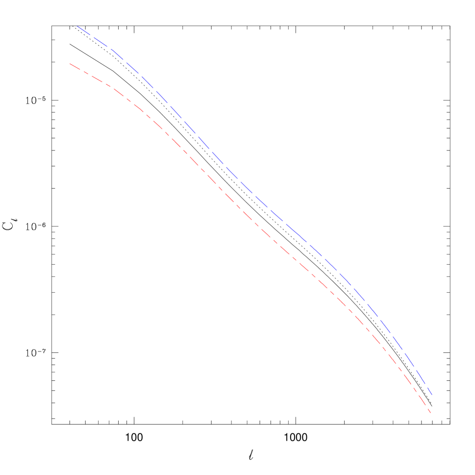
Figure 3: The dependence of the power spectrum on varying $\sigma_{8}$ and $\Omega_{m}$ separately. The solid line is our reference vanilla model with $\sigma_{8}=0.9,\Omega_{m}=0.3$. The long dashed line is for $\sigma_{8}=0.8$, the short-long dashed line is for $\sigma_{8}=1.0$ and the dotted line is for $\Omega_{m}=0.25$.

The correlation function decreases with increasing $\sigma_{8}$, as a higher $\sigma_{8}$ means the generalized selection function broadens and moves its peak to higher redshift. The broadening gives more non-correlated clusters nearby any given cluster, in addition the biasing is weaker for high $\sigma_{8}$. The cluster power spectrum scales quite differently with $\sigma_{8}$ than the temperature correlation function. If one parameterizes $C_{l}$ as

$$C_{l}(\sigma_{8})=\sigma_{8}^{-\alpha(l)}f(l),$$ (19)

for $Y_{min}=1.7\times 10^{-5}$ and $\sigma_{8}=0.9$, $\alpha(\ell)$ ranges from around 2.7 for $\ell\sim 100$ to about 1.6 for $\ell\sim 6000$. Doubling $Y_{min}$ changes this range to 3.5 and 1.7 respectively (note the negative power of $\sigma_{8}$ which is different from the positive power scaling behavior of the SZ temperature power spectrum (Komatsu & Seljak KomSel01 (2001), Sadeh & Raphaeli SadRep04 (2004)).

In fact, the effect of changing $\sigma_{8}$ is somewhat smaller, as there are other constraints which must be satisfied when changing $\sigma_{8}$, for instance the observed and hence fixed number counts of clusters. One can include this constraint by requiring the number of clusters to remain fixed along with $\Omega_{m}$ for instance, and find the required scaling between $T^{SZ}_{*}$ and $\sigma_{8}$(Sadeh & Rephaeli SadRep04 (2004)). Allowing $\Omega_{m}$ to vary still gives a constraint using identical arguments to Huterer & White HutWhi02 (2002) (also see Evrard et al Evretal02 (2002)) who were considering the X-ray temperature: Fixing the number of clusters with a given $Y$ parameter (an observable) and allowing $T^{SZ}_{*},\sigma_{8}$ and $\Omega_{m}$ to vary gives the following (directly analogous to X-ray) scaling relation,

$$T^{SZ}_{*}\sim(\sigma_{8}\Omega_{m}^{0.6})^{-1.1}\;.$$ (20)

More precisely it will be $f_{gas}T^{SZ}_{*}$ on the left. The modeling parameter $T_{*}^{SZ}$ will be discussed in detail in the next section. This relation already suggests a strong degeneracy between the effects of changing $\sigma_{8},T_{*}^{SZ},\Omega_{m}$, see section §4.3 for more discussion on degeneracies.

4.2 Modeling Uncertainties

There are several parameters and functions that go into the theoretical predictions besides the cosmological parameters. These can be divided into those related to cluster properties independent of the SZ effect, and those related to the transformation from cluster mass to the observable $Y$ (equation 8). We will treat both of these in turn. For an SZ selected survey, uncertainties in modeling affect results by bringing objects into or out of the survey. As a result, uncertainties that have a large effect on the observational properties of the lowest mass clusters in the survey ($M_{vir}\sim 10^{14}h^{-1}M_{\odot}$) have the most impact.

Dark matter cluster properties: The cluster properties independent of the SZ effect used in the analytic prediction of $C_{l}$, equation 16, are the correlation function of the dark matter, the mass function, and the bias.

Dark Matter correlation function: The dark matter correlation function is quite well known, and can be obtained from the initial power spectrum via a transfer function (such as BBKS BBKS (1986) or Eisenstein & Hu EisHu97 (1997)) and then by implementing a nonlinear power spectrum prescription (such as Peacock and Dodds PD96 (1996) or Smith et al Smi02 (2003)). The vanilla model uses the more accurate recent fits, i.e., the nonlinear power spectrum fit by Smith et al and the Eisenstein & Hu transfer function (the latter is within 3% of the exact CMB power spectrum, M. White, private communication). We compare the case with the BBKS transfer function to the vanilla model, as it is still in use by many groups.

Mass conversions: Before defining the mass functions, it should be recalled that there are several different mass definitions in use. For SZ calculations, the mass-temperature relation usually involves the virial mass, but the popular mass functions usually are instead for some linking length or parameter $\Delta$ such that the mass inside a radius $r_{\Delta}$ is $\Delta$ times the critical density:

$$M_{\Delta}=\frac{4\pi}{3}\Delta\rho_{crit}r_{\Delta}^{3}=\int_{0}^{r_{\Delta}}4\pi r^{2}dr\rho(r)\;.$$ (21)

This mass can differ significantly from the virial mass (White Whi01 (2001)), which enters into the definition of $Y$, and conversion must be made between the virial mass and the mass appearing in the mass function. The way suggested in White Whi01 (2001) is to start by assuming an NFW (Navarro, Frenk and White NFW (1997)) mass profile, a fitting formula for this method is given in Hu & Kravtsov HuKra03 (2003). For instance, in an $\Omega_{m}=0.3$ universe, $M_{vir}/M_{200}\sim 1.3$ for a cluster with concentration 5. A 30% difference in mass is significant when one is attempt to make percent-level predictions! Masses enter the calculations in the $Y(M)$ relation, the mass function and the bias; consistent definitions or the relevant conversions are needed. We show in figure 5 the effect on the vanilla model from using $M_{200}$ rather than the appropriate masses in the $Y(M)$ relation and bias.

Mass Functions: We compare the effects on the angular power spectrum of the above two possibilities, using a less accurate transfer function and neglecting the mass conversion, and three commonly used mass functions in figures 4 and 5.

Mass functions

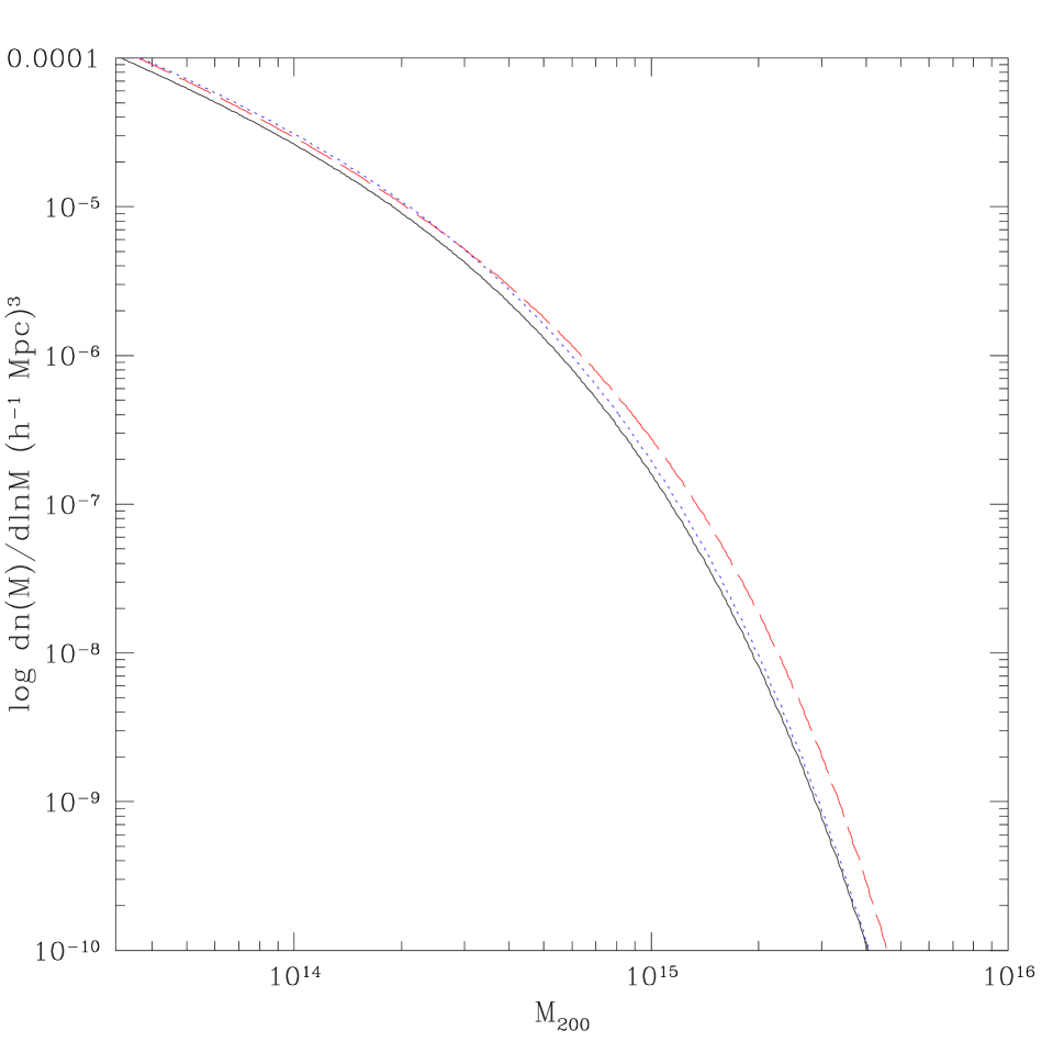
Figure 4: Evrard et al, Jenkins et al and Sheth-Tormen mass functions. The smooth line is the Evrard mass function, the dotted line is the Jenkins mass function and the dashed line is the Sheth-Tormen mass function.

Mass function dependence

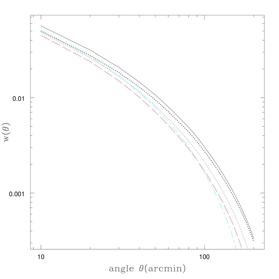
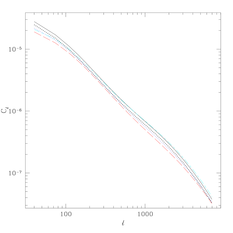
Figure 5: On left: The angular correlation function, same models and line labeling as figure 4, plus the vanilla model except for BBKS transfer function (dot-dashed line) and vanilla model without using mass function conversion for mass-temperature (heavy dotted line). On right: the corresponding angular power spectra.

The three mass functions taken here can be viewed as generalizations of the heuristic mass function of Press and Schechter PS (1974). These are based upon simulations with large enough volume to accurately sample the number of rare objects such as galaxy clusters: the Jenkins et al Jenetal01 (2001) mass function, the Sheth-Tormen SheTor99 (1999) mass function and the Evrard et al Evretal02 (2002) mass function. The first two are for masses in terms of $M_{180\Omega_{m}}$, while the last is in terms of $M_{200}$. These mass functions are expressed in terms of $\sigma(M,z)$ or $\nu(M,z)$. Here $\sigma(M,z)$ is the rms of the mass density field smoothed on a scale $R=(3M/(4\pi\rho_{b}))^{1/3}$ with a top hat window function, $\sigma(M,z)=\int^{\infty}_{0}\frac{dk}{k}\Delta^{2}(k)\tilde{W}_{M}^{2}(k,z)$ where $\tilde{W}_{M}^{2}(k,z)$ is the Fourier transform of window function, $\nu=\delta_{c}/\sigma$, and $\rho_{b}=\Omega_{m}\rho_{crit}$. We ignore the weak cosmological dependence of $\delta_{c}$ and set $\delta_{c}\equiv 1.686$. We then can write

$$\frac{dn}{dM}=\frac{\rho_{m}(z)}{M}f(\ln\sigma^{-1})\frac{d\ln\sigma^{-1}}{dM};$$ (22)

to get the three mass functions described in Table 1.

Table 1:

mass function	$\Delta\rho_{crit}$	$f(\ln\sigma^{-1}$)
Sheth-Tormen	$180\rho_{b}$	$\frac{0.364}{\sigma}(1+0.811\sigma^{0.6})e^{-\frac{1}{\sigma^{2}}}$
Jenkins	$180$ $\rho_{b}$	$0.301\exp[-|\ln\sigma^{-1}+0.64|^{3.82}]$
Evrard et al	$200$ $\rho_{crit}$	$0.22\exp[-|\ln\sigma^{-1}+0.73|^{3.86}]$

The mass density field and the correlation function are derived from the primordial power spectrum, which we take to be scale free, i.e. $n=1$, and normalized by $\sigma_{8}$. To get a sense of the effects, the (less accurate) earlier BBKS BBKS (1986) transfer function decreases $C_{\ell}$ by 5% at $\ell=214$, Neglecting the mass conversion between $M_{200}$ and $M_{vir}$ decreases $C_{214}$ by 11% and the Sheth-Tormen mass function SheTor99 (1999) decreases it by 19%. Using the Peacock & Dodds PD96 (1996) nonlinear prescription gives no noticeable change, hence we did not show it in the figure. An extensive comparison of different cases is given in the table in section §4.3.

Bias: There are also several different possibilities for bias. The (linear) bias $b(M,z)$ is defined via

$$\xi(M,M,r,z)=b^{2}(M,z)\xi(r,z)$$ (23)

where $\xi(r,z)$ is the dark matter power spectrum and $\xi(M,M,r,z)$ is the power spectrum of halos of mass $M$. The original idea of peak biasing by Kaiser biasedKaiser (1984) has been improved upon with fits to simulations. There is the Sheth-Tormen bias SheTor99 (1999), fit to simulations and motivated by a moving wall argument, the bias found by Sheth, Mo & Tormen SheMoTor01 (2001) (SMT), and the bias more recently found by Seljak and Warren SelWar04 (2004). The Seljak and Warren bias was found for small masses but has the best statistics currently available. It overlaps closely with the Sheth-Tormen bias where it is valid but is systematically lower and does not extend very far into the high mass range needed for clusters. Thus, using a combination of the two biases would result in a bias which doesn’t integrate to one when combined with the Sheth-Tormen mass function. Consequently we have taken the Sheth-Tormen bias as our default.

Table 2:

bias function	$\Delta\rho_{crit}$	bias
Sheth-Tormen	$180\rho_{b}$	$1+\frac{1}{\delta_{c}}(\nu^{{}^{\prime}2}-1)+\frac{2p}{\delta_{c}(1+\nu^{{}^{\prime}2p})}$
		$\nu^{\prime}=\sqrt{0.707}\delta_{c}/\sigma=1.418/\sigma,\;p=0.3$
Sheth, Mo & Tormen	$180\rho_{b}$	$1+\frac{1}{\delta_{c}}\left[\nu^{\prime 2}+b\nu^{\prime 2(1-c)}-\frac{\nu^{\prime 2c}/\sqrt{a}}{\nu^{\prime 2c}+b(1-c)(1-c/2)}\right]$
		$a=0.707,b=0.5,c=0.6$
Seljak & Warren	$200\rho_{crit}$	$0.53+0.39x^{0.42}+\frac{0.08}{40x+1}+10^{-4}x^{1.7}$
		$x=M/M_{nl}\;\;M=M_{nl}\leftrightarrow\nu=\sigma$

For the SZ selected power spectrum one integrates over all masses greater than some $M_{min}(Y_{min},z)$, so that what one is actually probing is an integral of the bias, i.e. $\Phi(Y_{min},z)$ in equation 14. One can define a related (rescaled by the number density) quantity:

$$b_{method,eff}=\frac{\int_{M_{min}(Y_{min})}^{\infty}dM\frac{dn}{dM}(z(r))b_{method}(M,z(r))}{\frac{dn}{dm}(z(r))}$$ (24)

where $b_{method}$ is one of the above biases. The linear biasing prescription above doesn’t work as well for short distances, and for this a “scale dependent bias” has been calculated for the cluster correlation functions by Hamana et al Hametal01 (2001) and Diaferio et al Dia03 (2003). This scale dependent bias is also a function of the separation $r$ of the objects of interest and for Diaferio et al is

$$b_{eff}(r,z,Y_{min})=b_{ST,eff}(z,Y_{min})(1+b_{ST,eff}(z,Y_{min})\sigma(r,z))^{0.35}$$ (25)

the corresponding expression for Hamana et al has an exponent 0.15. Diaferio et al have shown that this bias works well for cluster correlation functions for a range of redshifts. We will use the Diaferio et al case for illustration. The bias of Hamana et al is midway between the linear biasing case and the Diaferio et al case Dia03 (2003). With the Diaferio et al bias, the correlation function becomes

$$\begin{array}[]{ll}w(\theta)&=\int^{\infty}_{0}r_{1}^{2}\Phi(r_{1})\int^{\infty}_{0}r_{2}^{2}dr_{2}\Phi(r_{2})\tilde{\xi}_{dm}({|r_{1}-r_{2}|})\\ \end{array}$$ (26)

where

$$\tilde{\xi}_{dm}({|r_{1}-r_{2}|})=(1+b_{ST,eff}(z,Y_{min})\sigma(r,z))^{0.70}\xi_{dm}({|r_{1}-r_{2}|})$$ (27)

In the Limber approximation one then finds

$$w(\theta)=\int dyy^{4}\Phi(y)^{2}\int dx(1+b_{ST,eff}(z,Y_{min})\sigma(\sqrt{y^{2}\theta^{2}+x^{2}},z))^{0.70}\xi_{dm}(\sqrt{y^{2}\theta^{2}+x^{2}})$$ (28)

As this doesn’t easily allow a rewriting in terms of $J_{0}(\ell\theta)$, obtaining the power spectrum $C_{\ell}$’s is somewhat more difficult. In figure 6 we show the correlation function $w(\theta)$ at left and the power spectrum $C_{\ell}$ at right for the vanilla model and then the Sheth, Mo & Tormen linear bias and the Diaferio et al nonlinear bias. (Although the Hamana et al bias is also between the Diaferio et al bias and the vanilla bias, it is not what is shown in this figure.) We transformed the difference of $w(\theta)$’s between the vanilla model and Diaferio et al model to get the $C_{\ell}$’s for the former. We use the vanilla model parameters for the Diaferio et al bias (e.g. $T_{*}^{SZ}=1.2$ rather than $T_{*}^{SZ}=2.0$ as they did).

Bias dependence

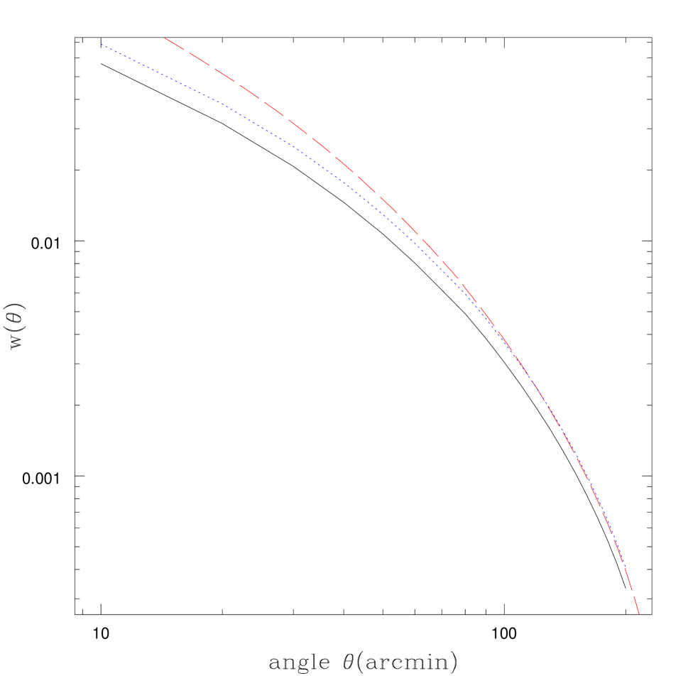
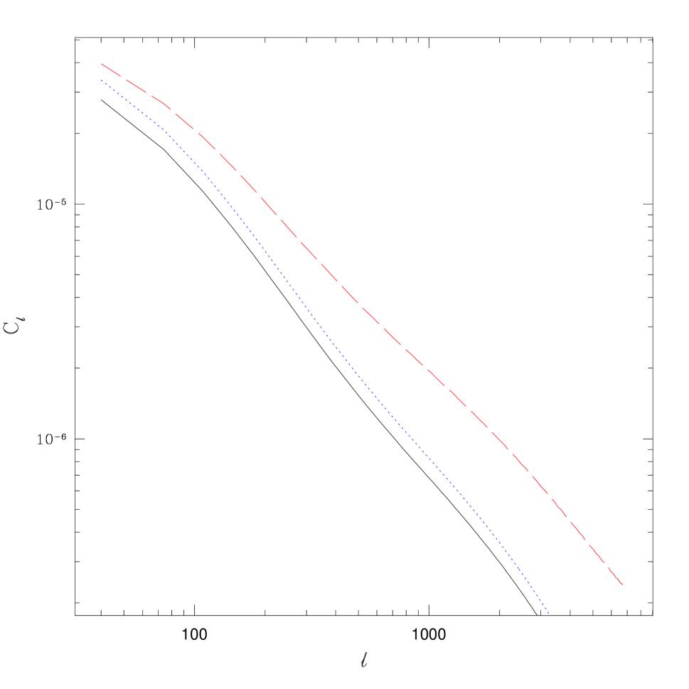
Figure 6: The effect of different bias prescriptions on the correlation function $w(\theta)$ (left) and the power spectrum $C_{\ell}$ (right). The vanilla reference model is shown in both cases (solid line), as well as the cases with the Sheth Mo & Tormen bias in equation 2 (dotted line) and the nonlinear bias of Diaferio et al, equation 25 (dashed line).

The nonlinear bias has the strongest effect at short distances in the correlation function–its effect is strongly localized around $\theta\sim 0$. Therefore its Fourier transform, the angular power spectrum, has additional contributions of almost constant magnitude at all $\ell$ relative to the vanilla model. (The limit of this would be adding power at only $\theta=0$, which translates into adding a constant to the power spectrum.) Some of this difference is deceptive as the errors for $C_{\ell}$ are independent in the linear regime, while those for $w(\theta)$ combine the $w(\theta)$ measurements for different values of $\theta$. For a visual comparison, the independence of the errors for $C_{\ell}$ makes it easier to draw conclusions about relations between different parameter choices and uncertainties. Also, even though the power spectrum and the correlation function are Fourier transform pairs, estimators for these differ in practice when real data is in hand, and give different information when one does not have full $2\pi$ angular coverage in $\theta$. Ideally one would use both given real data.

There is also intrinsic scatter around the bias and the mass functions. We will not put this in explicitly, however the weak dependence on the scatter in the $Y(M)$ relation (mentioned below) leads us to suspect it will not be a large effect.

$Y$ parameter: The next step is relating the cluster mass to a $Y$ parameter, which involves more complicated gas physics. In addition, the increased sensitivities of upcoming experiments will allow smaller and smaller mass clusters to be detected, which are more and more easily disrupted by this gas physics.

There are actually three questions: the actual form of the mass temperature/$Y$ parameter relation, the normalization of this relation (i.e. $T^{SZ}_{*}f_{gas}$) and the scatter around this normalization for a representative group of galaxy clusters. Simulations alone cannot determine these: the heating and cooling properties of clusters are not understood at an accuracy needed for precision cosmology and so these questions are intermingled by assumptions used. For instance, the scaling relation was obtained by assuming an isothermal gas profile. Assuming hydrostatic equilibrium and using the total $Y$ parameter means that the details of the profile (many others have been suggested, e.g. Komatsu & Seljak KomSel01 (2001), Loken et al Lok02 (2002)) get absorbed into the mass temperature (or $Y$ parameter) normalization or form. If the parameters of the gas profile change with cosmology, it’s possible that the normalization will also do so, or rather the form of the $Y(M)$ relation, a possibility which will need to be checked for carefully in the data. We consider the form of the mass temperature/$Y$ parameter relation, the normalization, and the scatter in turn.

Mass temperature/$Y$ parameter relation: There are several different mass temperature relations in the literature (see Sadeh & Rephaeli SadRep04 (2004) for a description of five common ones), usually based on X-ray mass temperature relations. These relations have been tested both with observations and simulations (bear in mind again that the simulations do not seem to yet have all the necessary physics), and some generalizations of these relations have also been tested. For instance, equation 8 can be generalized to include different $z$ and $M$ dependence, such as multiplying by a factor $(1+z)^{\gamma}M^{\alpha}$. The mass-Y parameter relation also has dependence on $f_{gas}$ which can be generalized to change $f_{gas}$ with redshift, or change it differently with mass. Observational data and simulation data have been used to search for these effects.

Most observational tests are of the X-ray mass temperature relations and of the change of $f_{gas}$ with mass or redshift, rather than of the $Y(M)$ relation. For example, Ettori et al 2004a have found no evidence for additional evolution in redshift of the mass temperature relation. For scaling of mass with temperature, Ettori et al 2004b and Ota & Mitsuda OtaMit04 (2004) find $T^{X-ray}_{gas}\sim M^{2/3}-M^{3/5}$, but the departure from the $M^{2/3}$ relation is about 1.5$\sigma$ for the Ettori et al data and is marginal given the error bars for the Ota & Mitsuda data. The former group also finds marginal (less than $2\sigma$) evidence for clusters of a fixed temperature to have smaller gas mass at high redshift. We have already included the $f_{gas}$ dependence with mass found by Lin et al LinMohSta03 (2003), but have not included any redshift dependence.

More simulations than observations have addressed the $z$ and $M$ dependences of the $Y(M)$ relation directly. For example da Silva et al daS04 (2004) find numerically that the $z$ dependence seems to be well represented by the simple scaling given in equation 8. For lower mass objects da Silva et al daS04 (2004) find that the $M$ dependence in the $Y(M)$ relation steepens from $M^{5/3}$. Our use of an $M$-dependent $f_{gas}$ produces an effect in the same direction. However, for clusters with $M_{200}$ above $5\times 10^{13}h^{-1}M_{\odot}$ (or $M_{vir}>6.5\times 10^{13}h^{-1}M_{\odot}$), one finds that this can just be absorbed into scatter of about 10 % around the $M^{5/3}$ scaling (White et al WhiHerSpr02 (2002)) in the $Y(M)$ relation. The effects of adding an additional factor of $(1+z)^{\gamma}M^{\beta}$ to $Y(M)$ has been considered for the angular correlation function by Moscardini et al Mos02 (2002) and Mei & Bartlett MeiBar03 (2003), and Wang et al Wan04 (2004) and Majumdar & Mohr MajMoh03 (2003, 2004) have considered the effects of this additional scaling on parameter estimation from the the power spectrum (the three dimensional one in the former case).

Normalization of $Y(M)$ relation: For normalization, we have combined all the mass temperature conversion ignorance into the parameter combination $Y\propto T^{SZ}_{*}f_{gas}$. The simplest procedure would be to say that $Y=Y_{vir}$ (and that gas outside this radius does not contribute significantly) and to take $T^{SZ}_{*}$ to be the X-ray value,

$$T_{*}^{SZ}\equiv T_{*}^{X-ray}\;.$$ (29)

As noted in section §2, there is strong disagreement between simulations and observations for $T_{*}^{X-ray}$. Thus the parameter $T_{*}^{X-ray}$ is not well determined. Even if it were, using it to normalize the $Y(M)$ relation is not necessarily justified. Not only do X-ray measurements weight more strongly the center of the cluster, as mentioned before, but for the SZ effect the normalization has an additional contribution due to line of sight contamination from gas outside the cluster. If one takes simulation results (which should be taken with a grain of salt given the above mentioned discrepancy), this projection effect on $Y(M)$ raises the normalization about 8% (White et al WhiHerSpr02 (2002)) above the normalization due to the cluster alone.

The differences between power spectra for different normalizations of the $Y(M)$ relation are shown in figure 7. We also show that taking $f_{gas}$ fixed at 0.06 $h^{-1}$ (the value for a cluster with $M_{vir}=10^{14}h^{-1}M_{\odot}$) gives a power spectrum very close to the vanilla model. And we additionally have shown a model with $T_{*}^{SZ}=2.2$keV which has the 8% increase from line of sight projection (from $T_{*}^{SZ}=2$keV).

Y(M) and mass-temperature normalization dependence

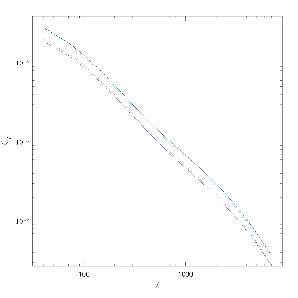
Figure 7: The power spectrum for the vanilla model, with $T_{*}^{SZ}=1.2$keV (solid line), and that with $T_{*}^{SZ}=2.0$keV (dotted line) as might be suggested by X-ray measurements. A higher value, $T_{*}^{SZ}=2.2$keV (dashed line) is also shown to give an idea of the change that an expected SZ line of sight projection effect (around 8%) would give. The dot-dashed line fixes $T_{*}^{SZ}=1.2$keV but has no evolution in $f_{gas}$ with mass, i.e. $f_{gas}=0.06h^{-3/2}$, the value for $M_{vir}=10^{14}h^{-1}M_{\odot}$.

Of course, as changing $T_{*}^{SZ}f_{gas}$ just rescales the $Y$ parameter, raising $T_{*}^{SZ}f_{gas}$ is equivalent to lowering $Y_{min}$, i.e. one is probing clusters with smaller mass.

Scatter: Unlike the normalization, the effect of scatter on the $Y(M)$ relation was very weak. Taking a 10-12% intrinsic scatter in the mass temperature relation (from Evrard, Metzler & Navarro EvrMetNav96 (1996) for X-ray simulations and similarly from White et al WhiHerSpr02 (2002) for SZ simulations) had less than a percent effect on the $C_{\ell}$, even with APEX sensitivity and accompanying very low mass cuts. For a large scatter of about 30%, $C_{\ell}$ was roughly decreased by about 3%. A similar robustness to M-T scatter was found in the Fisher matrix calculations (Levine, Schulz & White LevSchWhi02 (2002)) and in that of number counts (Battye & Weller BatWel03 (2003)). Metzler Met98 (1998) also found from simulations that the scatter in the mass temperature relation was larger than that for the mass-Y parameter relation. Thus for the bulk of the paper, we have used equation 8 and combined all our ignorance into the parameters $T^{SZ}_{*}f_{gas}$. We included the unnoticeable 10% scatter in the Y(M) relation in all our calculations here.

We were concerned about sources of scatter which are not included in our analytic description, mergers in particular. One might expect that processes such as merging will disrupt the clusters and thus invalidate the assumption of virialization used in some analytic calculations. The most massive clusters have the most recent mergers (as they are generally the most recently formed objects), but these tend to be included automatically in the catalogue as their estimated masses, even if inaccurate, are quite high relative to the mass cut. The selection for the catalogue depends most sensitively on the least massive clusters included, where mergers are relatively rarer. (However, at high redshift the “low mass” clusters are recently formed as they are the most massive collapsed objects at that time, so one might expect some effect from them.) Mergers are automatically included in the cosmological simulations and the scatter in the $Y-M$ relation is not larger than that expected due to scatter in the $M-T$ relation (White et al WhiHerSpr02 (2002)), leading us to expect that merger induced scatter is relatively small. However, as simulations cannot reproduce cluster properties precisely yet, observational data will be needed to calibrate this effect.

4.3 Degeneracies

We have considered several different choices for theoretical inputs to the calculations of the angular power spectrum. With a brief visual inspection it can be seen that there are many degeneracies, i.e. that several changes to parameters and modeling seem to have the same effect on the power spectrum. Note that this does not take into account other constraints at the same time, such as fixed number counts, only one parameter is varied at a time. We show some of these degeneracies more explicitly in figure 8,

Degeneracies

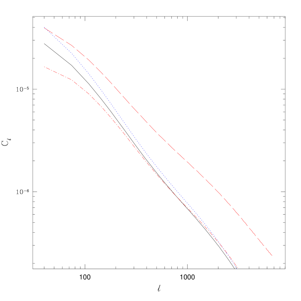
Figure 8: Degeneracies in theoretical modeling: On left, the center line is “vanilla” model, the 3 lower lines correspond to $\sigma_{8}=0.97$ (dotted), Jenkins Jenetal01 (2001) mass function (dot-dash), and $T_{*}^{SZ}=1.7$keV (dashed), and the 3 upper lines correspond to $\sigma_{8}=0.83$ (dotted), Sheth-Mo-Tormen SheMoTor01 (2001) bias (dot-dash), and $T_{*}^{SZ}=0.9$keV (dashed). On right, models which are not as degenerate. The solid line is “vanilla” model, the lower dot-dashed line is the (less accurate) BBKS transfer function, the upper dotted line is $\Omega_{m}=0.25$ and the top dashed line is the Diaferio et al nonlinear bias.

there are other degeneracies in the parameters considered here that aren’t shown. For instance, choosing a constant $f_{gas}$ rather than having evolution with mass, as done in the previous subsection, is degenerate with changing $T_{*}^{SZ}$ from 1.2 keV to 1.3 keV, using the Sheth-Tormen mass function rather than the Evrard mass function is degenerate with changing $T_{*}^{SZ}$ from 1.2 keV to 1.3 keV, and neglecting the mass conversion from $M_{200}$ to $M_{vir}$ and $M_{180\rho_{b}}$ in the $Y(M)$ relation and bias respectively is roughly degenerate rescaling $C_{\ell}$ overall by a factor of 0.88.

This can be compared to changing $\Omega_{m}$ or using the nonlinear bias of Diaferio et al, or using a less accurate transfer function such as BBKS, all of which change the “shape” of $C_{\ell}$ differently than those above. These are shown on the right of figure 8.

Values of $C_{\ell}$ for these models are compared quantitatively in the table 3.

Table 3:

Model	$C_{214}/10^{-6}$	$C_{1019}/10^{-7}$	$C_{4132}/10^{-7}$
vanilla	$4.75$	$6.67$	$1.00$
$T_{*}=0.9{\rm keV}$	$5.58$	$8.04$	$1.18$
$\sigma_{8}=0.83$	$5.80$	$8.04$	$1.17$
SMT bias	$5.75$	$8.10$	$1.21$
$T_{*}=1.7{\rm keV}$	$3.93$	$5.37$	$0.82$
$\sigma_{8}=0.97$	$3.98$	$5.66$	$0.87$
ST mass	3.87	4.89	0.79
Jenkins mass	4.13	5.42	0.86
no $f_{gas}$ evol	4.44	6.25	0. 93
no M conversion	4.16	5.89	0.88
BBKS	4.74	6.67	1.00
Diaferio bias	9.46	1.91	4.28
$\Omega_{m}=0.25$	5.60	7.56	1.06

The fact that $\Omega_{m}$ is not as degenerate with $\sigma_{8}$ as expected shows the limitations of the rough scaling estimate made in section §4.1. Some of these degeneracies can be broken by other measurements, for instance $dN/dz$, however the degeneracies are very similar, except for the bias. The bias has no effect on $dN/dz$ and thus can be taken out easily. In figure 9, we show $dN/dz$ for the same models considered for figure 8 (note that we are considering a full steradian).

Degeneracies $dN/dz$

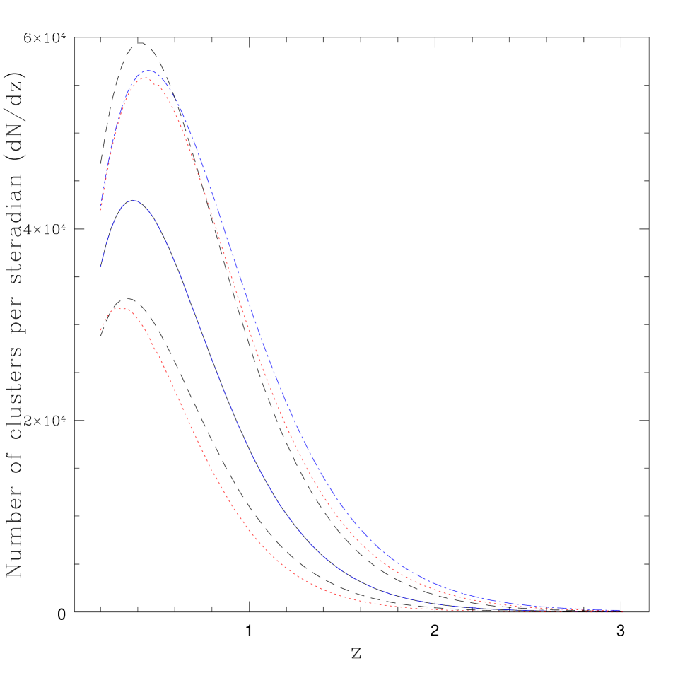
Figure 9: Degeneracies in theoretical modeling for dN/dz: labeling is the same as figure 7 left, except that the upper and lower groups of lines have switched. In addition, changing the bias to that of Sheth-Mo-Tormen has no effect on $dN/dz$ and so that line is now degenerate with the vanilla case.

As we have shown how choices like the mass function and different biases are degenerate with other parameter choices (in most cases), one is only as well measured as the other is known. In order to see how close these power spectra are in practice, we now compare to the inherent statistical measurement error.

4.4 Cosmic variance, sample variance and shot noise

There are three sources of inherent statistical measurement error for the power spectrum $C_{\ell}$ in the absence of any systematic errors: shot noise, cosmic variance and sample variance. These can be combined to give the standard expression for overall error (see, for example, Knox Kno95 (1995)):

$$\delta C_{\ell}=\sqrt{\frac{2}{(2\ell+1)f_{sky}}}\left(C_{\ell}+\frac{1}{\bar{n}}\right)\;.$$ (30)

The factor of $2\ell+1$ is due to the $2\ell+1$ independent measurements of the power for any $\ell$. For small $\ell$ (large scales) there are very few independent measurements of power in the sky, which is dubbed cosmic variance. Sample variance increases the error as the sky coverage $f_{sky}\leq 1$ decreases. Shot noise is determined by $\bar{n}$, the number density of clusters per steradian.

As the depth of the survey goes up ($Y_{min}$ decreasing), the power spectrum also decreases, as there are more and more clusters of lower and lower mass, and these are less correlated. However, the shot noise also goes down. On the other hand, as the depth of the survey decreases ($Y_{min}$ increasing), the power spectrum becomes restricted to higher and higher mass objects and thus goes up. However as these objects are rarer, the shot noise also increases. We can compare the errors quantities for 3 examples, APEX, SPT, and Planck.

We use the vanilla model and again take $Y_{min}=1.7\times 10^{-5}$ corresponding to a 5$\sigma$ detection for APEX with $\delta T\sim 10\mu$K (at 150 GHz). APEX will survey 100/200 square degrees at two frequencies (214 and 150 GHz, corresponding to 1.4 and 2 mm wavelengths), with 0.75’ resolution. For SPT, we expect about 4000 deg² and similar sensitivity and resolution. For Planck, we have all sky and will take a rough estimate of $Y_{min}=10^{-4}$ (sensitivity/resolution ranging from 5$\mu$K at 7.0’ to 50$\mu$K at 33.0’, depending upon frequency). First we plot the errors due to shot noise, sampling and cosmic variance for the Planck specifications above in figure 10.

Planck naive errors

Figure 10: The angular power spectrum with errors from shot noise, sampling and cosmic variance error expected from Planck, for a $Y_{min}=10^{-4}$. The bin size is the spacing between the error bars, equal spacing in log $\ell$. See text for more details.

Area vs. sensitivity

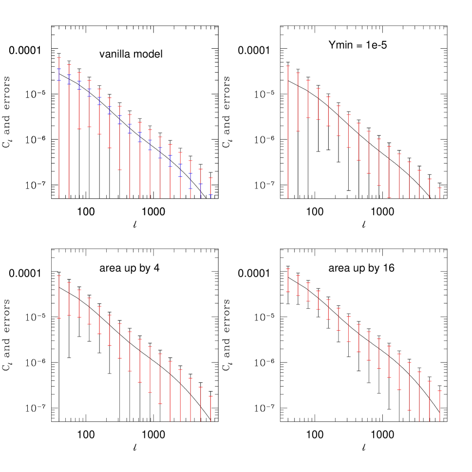
Figure 11: The angular power spectrum with errors from shot noise, sampling and cosmic variance error. Error bars are for 100, 200 and 4000 square degrees for the top two plots (vanilla model at left, $Y_{min}=10^{-5}$ at right), with the largest error bars corresponding to the smallest area. The lower figures correspond to the vanilla model except for the change $Y_{min}\rightarrow 2Y_{min,vanilla}$ ($4Y_{min,vanilla}$) on the left (right), with the area going up by a factor of 4 (16), relative to the vanilla model at upper left. This naively keeps the observing time fixed. The error bars are equally spaced in log $\ell$. See the text for more details.

In comparison, those for APEX and SPT are shown in figure 11. The vanilla model has the same parameters as earlier (including $Y_{min}=1.7\times 10^{-5}$), and error bars are shown for 100, 200, and 4000 square degrees, representative areas for data sets expected from APEX and SPT. The largest error bars are for the smallest area. The plot on the upper right has the same observing area, but with a minimum $Y_{min}$ value of $10^{-5}$. This might occur if e.g. $T_{*}^{SZ}$ were 2.0 keV rather than 1.2, a reasonable possibility given X-ray measurements and line of sight contamination effects. The sensitivity is directly proportional to $Y_{min}$, so “in principle” an experiment can fix $area/Y_{min}^{2}$ for a given observing time, producing a tradeoff between wide and shallow or narrow and deep. The errors given in equation 30 are shown for the vanilla model correlation function and then compared to other possibilities with fixed observing time. Note this ignores how the efficiency and difficulty of cluster identification changes with $Y_{min}$. The errors also neglect the Poisson nature of the shot noise and the 3 and 4 point functions of the clusters, thus we are calling them “naive”. The bottom two graphs are the vanilla model plotted with a smaller $Y_{min}$ with error bars corresponding to the 100 and 200 square degree surveys with area up by the factor of 4 or 16 for the left and right graphs respectively. Note that as the sensitivity goes down that the power spectrum and the shot noise go up, as mentioned earlier–only rarer and thus more clustered objects are included. The bin size is the spacing between the error bars, equal in log $\ell$. However, the decrease in error bars due to increased sky coverage outweighs the increase in shot noise: shallow and wide appears naively preferable to deep and narrow.

In fact, poorer sensitivity is not necessarily a bad thing, as the omitted clusters have low mass and thus the strongest dependence on the poorly understood gas physics. Exactly how deep is the most profitable will depend very strongly on the normalization of the $Y(M)$ relation. In addition, the corresponding changes in the purity and completeness of the surveys have not been taken into account in this scaling argument, how these properties scale will depend upon the cluster finding algorithms in use as well. Fixing the sensitivity and increasing the area, as SPT will do, is of course a major improvement in any case.

In addition, even though the error bars are quite large, the measurement contains useful information. Theory gives smooth and known functions of $\ell$, $C_{\ell}$, so we can bin $N_{\ell}$ nearby values of $\ell$, reducing the error. For example, we can use the combined shape of the power spectrum (20 bins equally spaced in log $\ell$) and the errors in equation (30) to find one sigma contours in the $\sigma_{8}-\Omega_{m}$ plane. This is shown in figure 12 for marginalizing over a 10% prior and a 30% prior on $T_{*}^{SZ}$ and holding all the other uncertainties fixed for our “vanilla” model.

Figure 12: The one sigma contours using the full power spectrum and errors in equation (30), varying $\Omega_{m}$ and $\sigma_{8}$, marginalized with a 10% prior on $T_{*}^{SZ}$ (left) and a 30% prior on $T_{*}^{SZ}$ (right). The larger contour is for 200 square degrees (APEX) and the smaller one is for 4000 square degrees (SPT). The true model is our “vanilla” model, shown by the point at the center.

These error ellipses clearly illustrate the degeneracies inherent in the effects of changing these two cosmological parameters for the angular power spectrum. The closest error analysis to ours was done by Mei and Bartlett MeiBar04 (2004) who used the measurement of $w(\theta)$ at 30 arcminutes and counts at the flux limit to get error contours for $\sigma_{8}$ and $\Omega_{m}$ of comparable size. Here instead we use the full power spectrum because our intent is to illustrate the degeneracies in using the power spectrum to constrain these parameters. As Mei and Bartlett’s degeneracy line in $\Omega_{m},\sigma_{8}$ for $w(30^{\prime})$ differs from the ellipse axes in figure 12, the two sets of constraints are complementary.

5 Conclusions

Forthcoming SZ surveys such as APEX are expected to observe one or two orders of magnitude more clusters than currently in hand. The angular power spectrum will be an immediate result once clusters have been identified. There still exists uncertainty in theoretical predictions: we examined how those uncertainties affect the cluster power spectrum.

We calculated the angular power spectrum for different reasonable mass functions, biases, mass-temperature normalizations $T_{*}^{SZ}$ and gas fractions $f_{gas}$ and found these changes are comparable to changes due to cosmological parameters of interest such as $\sigma_{8}$ within current ranges of interest. In particular we identified which modeling uncertainties mimicked changes in the cosmological parameters considered (by finding the relevant cosmological parameter values) and which did not. Some of these modeling and cosmological dependencies have been studied for the correlation function in two dimensions or the three dimensional power spectrum. Different subsets with different fixed assumptions have been considered in previous literature at different times. By combining all these variations in a homogeneous manner, and including several more which have been identified since, the relative importance of the various modeling assumptions can be more directly assessed.

We find that progress on several fronts is needed before the scientific harvest from these experiments can be fully realized.

The uncertainties in the mass function of clusters and the bias can both be improved with simulations. We showed the differences between many commonly used ones are significant in comparison to the uncertainties for the cosmological parameters of interest.

We have summarized much of the observational and theoretical work on the $Y(M)$ relation, important uncertainties still remain. The normalization of the $Y(M)$ relation needs considerable observational and/or simulation input (this point has also been emphasized previously by other authors as referenced in the text). Current experiments such as SZA might be able to do this calibration when combined with other measurements for mass, as long as the normalization is not redshift dependent. Simulations with gas are known to have incomplete treatments of physics but can be used as a guide, e.g. to calibrate the effect of projection on the mass temperature relation, which gives a systematic increase of the $Y(M)$ normalization of about 8%. We included scatter in the $Y(M)$ relation, however this was a small effect: the angular power spectrum changed by less than 1% when the $Y(M)$ relation was taken to have a scatter (as recent hydrodynamic simulations suggest) of 10%. The effects of mergers seem to be small, once the normalization is fixed; we argue that the effect of most of the parameters is just to decide whether objects are included in the survey or not, and mergers have the largest effect on the largest clusters, which tend to be included anyhow for the low values of $Y_{min}$ under consideration here.

We also studied the experimental uncertainties which exist even in the absence of systematic uncertainty. We compared area to sensitivity $Y_{min}$ and found that naively a shallower wider survey is more powerful.

We focused on the angular power spectrum alone, though of course complementarity is key to progress. Complementary data will even be provided from survey producing the power spectrum itself. A survey providing an angular power spectrum will also produce number counts per square degree and $dN/dY$, number counts as a function of $Y$. In addition, the temperature correlation function and perhaps $dN/dz$ will be available. Various combinations of these quantities have been analyzed in the literature. Mei and Bartlett considered number counts and the angular correlation function, and combined it with the number counts from X-ray, for instance. This is one example of self-calibration (Levine, Schulz & White LevSchWhi02 (2002)); adding the angular power spectrum to other measurements will increase the leverage of all of them.

J.D.C. thanks G. Evrard, A. Kravtsov, E. Reese and W. Hu for discussions and S. Mei for help with comparing with her work; K.K. thanks P. Zhang, W. Hu and J. Weller for useful discussions. We both especially thank M. White for numerous discussions, early collaboration on this project and comments on the draft, and the anonymous referee for many constructive suggestions. This work was supported in part by DOE, NSF grant NSF-AST-0205935 and NASA grant NAG5-10842.

References

- (1) Barbosa, D., Bartlett, J. G., Blanchard, A., Oukbir, J., 1996, A & A, 314, 13
- (2) Bardeen, J. M., Bond, J. R., Kaiser, N., Szalay, A. S.,1986, ApJ 304, 15
- (3) Bartlett, J.G., Silk, J., 1994, ApJ, 423,12
- (4) Bartlett, J.G., 2001, published on arXive as astro-ph/0111211
- (5) Battye, R. & Weller, J., 2003, Phys Rev D, 68, 3506
- (6) Birkinshaw, M., 1999, Phys.Rept. 310, 97
- (7) Borgani, S., et al, 2004, MNRAS 348, 1078
- (8) Carlstrom, J., Holder, G., Reese, E., 2002, Ann.Rev.Astron.Astrophys. 40, 643
- (9) Casas-Miranda, R., Mo, H.J., Sheth, R.K., Borner,G., 2002,MNRAS 333, 730
- (10) Cohn, J., 2005 [astro-ph/0503285].
- (11) da Silva, AC., Kay, S.G., Liddle, A.R., Thomas, P.A., 2004, MNRAS 348, 1401
- (12) Diaferio, A.,Nusser, A., Yoshida, N., Sunyaev, R., 2003, MNRAS 338, 433
- (13) Eisenstein, D., Hu, W., 1997, ApJ 511, 5
- (14) Ettori, S., Tozzi, P., Borgani, S., Rosati, P., 2004, A & A 417, 13
- (15) Ettori, S., et al, 2004, astro-ph/0407021
- (16) Evrard, A.E., Metzler, C., Navarro, J., 1996, ApJ 469, 494
- (17) Evrard, A.E., et al, 2002, ApJ 573, 7
- (18) Fan, Z.H., Wu, Y.L., 2003, ApJ 598, 713
- (19) Geisbusch, J., Kneissl, R., Hobson, M., astro-ph/0406190
- (20) Hamana, T., Yoshida, N., Suto, Y., Evrard, A.E., 2001,ApJ 561, L143
- (21) Holder, G. P., Mohr, J. J., Carlstrom, J. E., Evrard, A. E., Leitch, E. M., 2000, ApJ, 544, 629
- (22) Holder, G.P., Haiman, Z., Mohr, J.J., 2001, ApJ 560, L111
- (23) Hu, W., & Kravtsov, A., 2003, ApJ, 584, 702
- (24) Huterer, D. & White, M., 2002, ApJ, 578, 2.
- (25) Itoh, N., Kohyama, Y., Nozawa, S., 1998, ApJ, 502, 7
- (26) Jenkins, A., et al, 2001, MNRAS 321, 372
- (27) Kneissl, R., et al., 2001, MNRAS 328, 783
- (28) Knox, L, 1995, Phys.Rev.D, 52, 4307
- (29) Knox, L, Holder, G, Church, S, 2004, ApJ 612, 96
- (30) Komatsu, E., Kitayama, T., 1999, ApJ 526, L1
- (31) Komatsu, E. & Seljak, U., 2001, MNRAS, 327, 1353
- (32) Komatsu, E. & Seljak, U., 2002, MNRAS, 336, 1256
- (33) Kravtsov, A., 2005, private communication
- (34) Levine, E.S., Schulz, A.E., White,M., 2002, ApJ 577, 569
- (35) Limber, D.N., 1953, ApJ, 117, 134
- (36) Lin, Y.T., Mohr, J.J., Stanford, S.A., 2003, ApJ 591, 749
- (37) Loken, C., et al, 2002, ApJ 579, 571
- (38) Majumdar, S., Mohr, J.J., 2003, ApJ 585, 603
- (39) Majumdar, S., Mohr, J.J., 2004, ApJ 613, 41
- (40) Mathiesen, B. & Evrard, A.E., ApJ 546, 100
- (41) Mazzotta, P., et al, 2004, astro-ph/0404425
- (42) Mei, S., Bartlett, J., astro-ph/0407436
- (43) Mei, S., Bartlett, J., 2003, A & A, 410, 767
- (44) Melin, J.-B., Bartlett, J.G., Delabrouille, astro-ph/0409564, A & A to appear
- (45) Metzler, C., published on arXive as astro-ph/9812295
- (46) Metzler, C., White, M., Loken, C.,2001, ApJ 547, 560
- (47) Moscardini, L.; Bartelmann, M.; Matarrese, S.; Andreani, P., 2002, MNRAS 335, 984
- (48) Navarro, J. F., Frenk, C.S., White, S.D.M., 1997, ApJ 490, 493
- (49) Nozawa, S., et al, 2000, ApJ, 536, 31
- (50) Ota, N., Mitsuda, K., 2004, astro-ph/0407602, A & A to appear.
- (51) Peacock, J.A., Dodds, S.J., 1996, MNRAS 280L, 19
- (52) Pierpaoli, E., Anthoine, S., Huffenberger, K., Daubechies, I., astro-ph/0412197
- (53) Pierpaoli, E., Borgani, S., Scott, D. & White, M, 2003, MNRAS, 342, 163.
- (54) Press, W., Schechter, P., 1974, ApJ 187, 425
- (55) Kaiser, N., 1984, ApJ 284, L9
- (56) Rasia, E., et al, 2005, ApJ 618, L1
- (57) Rephaeli, Y., 1995, ARA & A 33, 541
- (58) Rephaeli, Y., 1995, ApJ 445, 33
- (59) Sadeh, S., Rephaeli, Y., 2004, New Astronomy, 9, p 373
- (60) Schulz,A.E., White,M., 2003, ApJ 586, 723
- (61) Seljak, U., Warren, M.S., astro-ph/0403698
- (62) Sheth, R., Lemson, G., 1999, MNRAS 304, 767
- (63) Sheth, R., Tormen, G., 1999, MNRAS 308, 119
- (64) Sheth, R, Mo, H.J. Tormen, G., 2001, MNRAS, 323, 1
- (65) Smith, R.E. et al, 2003, MNRAS 341, 1311
- (66) Sunyaev R. A. & Zel’dovich, 1972, Comm. Astrophys, Space Phy., 4, 173
- (67) Sunyaev R. A. & Zel’dovich, Ya. B., 1980, ARA&A, 18, 537
- (68) Tegmark, M., et. al, 2004, Phys.Rev. D69, 103501
- (69) Vale, C., White, M., 2005, astro-ph/0501132
- (70) Wang, S., Khoury, J., Haiman, Z., May, M., 2004, Phys.Rev.D70, 123008
- (71) White, M., 2001, A & A, 367, 27
- (72) White, M., Hernquist, L., Springel, V., 2002, ApJ 579, 16
- (73) White, M., Majumdar, S., 2004, ApJ 602, 565