Observational Tests and Predictive Stellar Evolution II: Non-standard Models

Abstract

We examine contributions of second order physical processes to the results of stellar evolution calculations which are amenable to direct observational testing. In the first paper in the series (Young, Mamajek, Arnett, & Liebert, 2001) we established baseline results using only physics which are common to modern stellar evolution codes. In the current paper we establish how much of the discrepancy between observations and baseline models is due to particular elements of new physics in the areas of mixing, diffusion, equations of state, and opacities. We then consider the impact of the observational uncertainties on the maximum predictive accuracy achievable by a stellar evolution code. The sun is an optimal case because of the precise and abundant observations and the relative simplicity of the underlying stellar physics. The Standard Model is capable of matching the structure of the sun as determined by helioseismology and gross surface observables to better than a percent. Given an initial mass and surface composition within the observational errors, and no current observables as additional constraints for which the models can be optimized, it is not possible to predict the sun’s current state to better than $\sim 7\%$. Convectively induced mixing in radiative regions, terrestrially calibrated by multidimensional numerical hydrodynamic simulations, dramatically improves the predictions for radii, luminosity, and apsidal motions of eclipsing binaries while simultaneously maintaining consistency with observed light element depletion and turnoff ages in young clusters (Young et al., 2003). Systematic errors in core size for models of massive binaries disappear with more complete mixing physics, and acceptable fits are achieved for all of the binaries without calibration of free parameters. The lack of accurate abundance determinations for binaries is now the main obstacle to improving stellar models using this type of test.

1 INTRODUCTION

Stellar evolution has become a successful tool for elucidating the processes at work in individual stars. New instrumentation and a wealth of new data has resulted in increased emphasis in astronomy on the evolution of galaxies over cosmic history. Obviously the stellar content of a galaxy plays a central role in its evolution. In order to understand this process, we require theoretical stellar evolution to be predictive, in the sense of being able to accurately describe the contribution of luminosity, kinetic energy, and nucleosynthetic products from a star of a specific initial mass and composition at any and all points in its life. This process must be able to be carried out self consistently for stars from the hydrogen burning limit to the highest possible masses, so that stellar outcomes can be reliably linked to an initial mass function (IMF). This is not possible with schemes which are adjusted to match astronomical observations. Without an underlying physical theory, the calibration cannot be reliably extrapolated to regimes without extensive and independent observational data. Also, multiple physical effects can contribute in opposite or orthogonal senses to the star’s structure. As an example, determinations of metallicity of binaries are often made by fitting model tracks of varying composition to observed points and finding the best fit. However, more mixing produces more luminous models for a given mass at a given effective temperature. Lower metallicity shifts tracks bluewards and slightly higher in luminosity. Either change could force a model to pass through the desired observed point. So a model with incomplete mixing physics and solar composition could be as good a formal fit to specific observations as a model with more complete physics and supersolar metallicity.

The two primary areas which strongly affect the evolution and have uncertain physics are mixing and mass loss. The evolution is also sensitive to the opacity of the stellar material, but the opacities used in evolution codes are largely uniform, utilizing the OPAL values of Iglesias & Rogers (1996) for high temperatures and Alexander & Ferguson (1994) for low temperatures. The observational errors in determining stellar compositions are the major limitation on further testing contribution of opacities to stellar models. Even the metallicity of the sun varies from z=0.019 (Grevesse & Sauval, 1998) to z=0.015 (Lodders, 2003), depending upon the precise physical assumptions and dimensionality of the codes being used to fit the measured line profiles. Most other test cases, such as most double-lined eclipsing binaries, have no published metallicity determinations using high resolution spectroscopy. Equations of state (EOS’s) are not uniform across stellar evolution codes. While the effects of the EOS are perhaps more subtle, they can still be important, particularly for low mass stars and pre- and post-main sequence evolution.

In Young, Mamajek, Arnett, & Liebert (2001), we presented baseline results from stellar models calculated using only physics common to current widely used stellar evolution codes. These models were tested against a subset of double-lined eclipsing binaries (Andersen, 1991; Ribas et al., 2000; Latham et al., 1996; Lastennet & Valls-Gabaud, 2002; Hillenbrand & White, 2004). Young et al. (2003) discussed hydrodynamic mixing within the radiative regions of stars and presented several observational tests of the mechanism. This paper presents a reanalysis of the eclipsing binary sample and solar models, with more realistic mixing physics as well as additional minor improvements to the code. Section 2 summarizes the additional physics and improvements to the code. Solar models are examined in Section 3. The eclipsing binary sample is presented in Section 4. Section 5 contains discussion and conclusions. The implications for post-main sequence evolution will be presented in a subsequent paper.

2 THE TYCHO CODE

The TYCHO code is a 1D stellar evolution and hydrodynamics code written in structured FORTRAN77 with online graphics using PGPLOT. The code is as described in Young, Mamajek, Arnett, & Liebert (2001). We have made substantial additions and improvements. The code is now functional for stars from the hydrogen burning limit to arbitrarily high masses, and for metallicities of z = 0 to the limit of the OPAL opacity tables.

The opacities used are from Iglesias & Rogers (1996) at high temperatures and Alexander & Ferguson (1994) for low temperatures. The OPAL tables have been extended to low entropies, and are formally adequate for calculating stellar interiors down to the hydrogen burning limit. In reality, a number of contributions, particularly from molecular species, are not included. Stellar models computed with these tables are reliable to perhaps 0.5 $M_{\odot}$.

TYCHO uses an adaptable set of reaction networks, which are constructed automatically from rate tables given a list of desired nuclei. In these calculations a 176 element network complete through the iron peak was used at $T>10^{7}$ K, and a 15 element network for light element depletion at lower temperatures. Rates for the full network are from Rauscher & Thielemann (2000). Caughlan & Fowler (1988) rates are used in the light element network.

Mass loss capabilities of the code have been extended. At $T_{eff}>7.5\times 10^{3}$K, the theoretical approach of Kudritzki et al. (1989) is used. At lower $T_{eff}$ routines based upon the empirical prescription of Dupree & Reimers (1987) or Blöcker (1995) are available. Low temperature mass loss was not important in any of the cases studied here, and the Reimers and Blöcker algorithms converge in the limit of low luminosity. A treatment of radiatively driven mass loss in Wolf-Rayet stars based upon the work of Lamers & Nugis (2003) is also included in the code. It does not come into play for these models and will be discussed in a separate paper.

The equation of state has been expanded from the modified Timmes & Swesty (2000) EOS in Young, Mamajek, Arnett, & Liebert (2001) to include a more generalized treatment of the coulomb properties of the plasma. The formation and dissociation of molecular hydrogen and its effect upon the equation of state are also included in a Helmholtz free energy formulation. The OPAL project has extended its EOS determinations to lower entropies. The improved TYCHO equation of state agrees with the OPAL EOS to better than 1% for most conditions. There remains a difficult region ($10^{-1}\leq\rho\leq 10^{1}{\rm g\ cm^{3}}$ and $T\leq 10^{5.5}$ K) in which the plasma is a strongly interacting coulomb system, and in which the difference exceed 4%. This region is relevant for low mass stars ($M<0.5M_{\odot}$).

TYCHO uses a modified version of Ledoux convection which avoids the problem of instantaneous mixing in convective regions with nuclear burning during short timesteps. Simple Eddington-Sweet rotational mixing (Tassoul, 2000) is implemented in the code. Rotation was not included in the binary models as these systems are all relatively slow rotators for their mass range. Based on test models, rotation seems to be a perturbation of the order of the observed errors or less on the observed quantities we are examining.

All models were run with an improved version of the inertial wave driven mixing described in Young et al. (2003). This treatment is primarily derived from Press (1981) and references therein. Press begins from two separate approximations to describe the propagation of internal waves in a stellar interior. The global behavior of the waves is described by the anelastic approximation (Ledoux, 1974). Boussinesq, plane equations with thermal diffusion describe the damping behavior of linear internal waves (Lighthill, 1978). Press (1981) combines these equations to define a set of globally anelastic but locally Boussinesq equations. The principal equation of motion is

$$\frac{\partial^{2}{\bf\Psi}}{\partial r^{2}}+\left(\frac{N^{2}}{\omega^{2}}-1\right)k_{H}^{2}{\bf\Psi}+\frac{i\sigma}{\omega}\left(\frac{\partial^{2}}{\partial r^{2}}-k_{H}^{2}\right)^{2}{\bf\Psi}=0$$ (1)

where

$${\bf\Psi}\equiv\rho_{0}^{\text@frac{1}{2}}k_{H}^{-2}u_{V},$$ (2)

$N$ is the composition dependent Brunt-Väisälä frequency,

$$N^{2}=-g\frac{1}{\rho_{0}}\frac{d\rho_{0}}{dz}-\frac{1}{\Gamma_{1}P}\frac{dP}{dr},$$ (3)

$k_{H}$ is the local horizontal wavenumber,

$$k_{H}\equiv\left[\frac{l(l+1)}{r^{2}}\right]^{\text@frac{1}{2}},$$ (4)

$\sigma$ is the thermal diffusivity,

$$\sigma\equiv\frac{4(\Gamma 1-1)}{\Gamma 1}\left(\frac{\text@frac{1}{3}aT_{0}^{4}}{P_{0}}\right)\left(\frac{c}{\kappa_{0}\rho_{0}}\right),$$ (5)

and $\omega$ is the characteristic frequency of the driving, in this case convective modes of low frequency. The vertical fluid velocity $u_{V}$ (for moderate damping) is determined from a WKB solution of equation 1, and the vertical wavenumber $k_{V}$ is defined as

$$k_{V}\equiv k_{H}\left[\frac{N^{2}}{\omega^{2}}-1\right]^{\text@frac{1}{2}}.$$ (6)

The quality factor $Q$ of the propagating waves is

$$Q=2\frac{N}{\sigma k_{H}^{2}}\left(\frac{\omega}{N}\right)^{3}\left(\frac{N^{2}-\omega^{2}}{N^{2}}\right).$$ (7)

Waves generated by the convective zone are in most circumstances non-linear within one linear damping distance of the convective zone. Mixing in this region is efficient, but it is a small fraction of the star. We are also interested in the impact of the waves outside this zone. Damping of the waves in the radiative region generates vorticity as described in Young et al. (2003). Press (1981) derives a mass diffusivity coefficient $\sigma_{M}$, which we adopt, as,

$$\sigma_{M}\sim\frac{\epsilon^{4}\sigma^{2}k_{V}^{2}}{\omega}\sim\sigma\frac{\epsilon^{4}}{Q}$$ (8)

where $\epsilon$ is the dimensionless nonlinearity parameter for internal waves

$$\epsilon\equiv\frac{k_{H}u_{H}}{\omega}.$$ (9)

The efficiency of the wave propagation, and therefore the mixing, is inherently sensitive to composition gradients through $N$ and, indirectly, through the opacity in $\sigma$. The mixing occurs roughly on a thermal timescale. It is slow relative to convective turnover, but it can be significant on evolutionary timescales. In practice, this drives mixing in what are typically referred to as “semiconvective” regions, where $(\frac{N^{2}}{\omega^{2}}-1)>0$. When this quantity becomes imaginary, the wave undergoes complete internal reflection, and there is an exponential falloff of the wave flux beyond this boundary. In terms of composition gradients, there is a region outside the convective zone which is well mixed, with a further sharply decreasing degree of mixing beyond. This treatment removes the one variable parameter from Young et al. (2003), the characteristic length for dissipation, by treating the wave physics more completely. Our results are little changed from the earlier formulation. This is unsurprising, as we constrained the earlier treatment with numerical simulations in which the wave behavior was readily apparent.

Gravitational settling and differential diffusion of nuclear species according to Thoul, Bahcall, & Loeb (1994) is also included. The Thoul, Bahcall, & Loeb (1994) treatment of diffusion is generalizable to an arbitrary number of nuclear species, though that work examines only H, He, O, and Fe. We calculate diffusion coefficients separately for the species important to the OPAL “type 2” opacity tables (H, He, C, and O) and on average for iron peak and Ne like elements. Michaud et al. (2004) examine the effect of settling on the approximately solar age and metallicity clusters M67 and NGC 188, using 19 elements. In light of these results our intermediate simplification appears adequate for stellar structure calculations.

Numerous minor improvements have been made which improve convergence and stability of the code, and allow it to perform adequately at the small timesteps typical of neutrino-cooling dominated burning stages as well as the slow hydrogen burning stages. The code is publicly available and open source. The current version (TYCHO-7.0) is being made available, along with an extensive suite of analysis tools, at http://pegasus.as.arizona.edu/$\sim$darnett.

3 SOLAR MODELS

As the best observed star in the sky, the Sun is an obligatory test case for any comprehensive stellar evolution code. The helioseismological measurements of sound speed and depth of the convective zone give us an insight into the interior structure not available for any other star. In this section we test solar models from TYCHO, but with a somewhat novel aim. We hope that TYCHO will function as a predictive tool for building stellar populations. Therefore, instead of finding a best fit to objects as they are observed now, with variable initial conditions, the code must be able to predict a unique (and accurate) path through stellar parameter space over time for a particular initial mass and composition. Conversely, we would also like to connect any given observed star to a unique initial condition. We would wish to do this for the complete range of stellar masses. As such we are more interested in the comparison of our models with the sun, assuming only an initial solar mass, composition, and our best treatment of the physics, than in how precisely we can fit the sun by optimizing our models. A 1 $M_{\odot}$ star on the main sequence is probably the easiest type of star to model, being relatively insensitive to the effects of mixing and mass loss. Solar models give us an estimate of the minimum uncertainty in our predictions of stellar parameters.

We examine four models, s0, s1, s2, and s3 which differ in the completeness of mixing physics included. Model s0 includes gravitational settling and diffusion (Thoul, Bahcall, & Loeb, 1994) and inertial wave-driven mixing (Young et al., 2003). Model s1 includes only wave-driven mixing and s2 only gravitational settling and diffusion. Model s3 uses only Ledoux convection and ignores other mixing physics. Eddington-Sweet mixing is disabled, as it is a poor description of the true angular momentum distribution in the sun. We also calculate one model (l0) with physics identical to s0, but with Lodders (2003) values for solar abundances.

There is one glaring limitation, a free parameter which must of necessity remain in this 1-D code. We choose a mixing length parameter of $\alpha=2.1$, where $\alpha$ is the ratio of the mixing length to the pressure scale height. This is in the same range as values deduced from solar standard models ($\alpha$ = 2.05) (Basu, Pinsonneault, & Bahcall, 2000) and multidimensional simulations of the solar convective zone with hydrodynamics and radiative transfer ($\alpha$ = 2.13)(Robinson et al., 2004). Smaller values of the mixing length parameter result in larger radii for the 1-D models. The mixing length parameter is a shorthand for more complex physics, and is not guaranteed to be constant over stellar mass or evolutionary state, so these constraints apply only to sun-like stars.

Table 1 gives values for gross observables ($R,T_{eff},L$), the rms difference in predicted and observed sound speed, depth of convection zone, photospheric He and Li values, and central temperature for each model. (Note that the observed Li abundance in the sun is much lower than the meteoritic value. The meteoritic value is assumed to more accurately represent the abundance in the proto-solar nebula, and as such is used as the starting value for the models.) We have not performed an inversion of the helioseismological data through our model to obtain expected sound speeds for our models. The values to which we compared are those calculated by Bahcall, Pinsonneault, & Basu (2001). We have roughly twice as many Lagrangian mass points as the online tables for the standard models, so we perform an interpolation in our sound speeds to match the standard model tables. Performing this direct comparison we find rms errors in sound speed of $\sim 0.5\%$ for our best models. Most of this discrepancy can be attributed to our error in the solar radius. (Bahcall, Pinsonneault, & Basu (2001) find a 0.15% rms error for a model with a 0.04% difference in radius from their standard value.)

Table 2 gives neutrino fluxes for the models and a selection of models from Bahcall & Pinsonneault (2004). The Bahcall & Pinsonneault (2004) model BP04 is the current standard solar model. BP04+ includes improvements in nuclear physics, solar equation of state, nuclear physics and solar composition. The entry “Comp” shows the effects of variant composition alone, and ${\rm N^{14}}$ shows the effects of a change in the ${\rm N^{14}}(p,\gamma){\rm O^{15}}$ rate alone.

Table 1: Characteristics of Solar Models with Varied Mixing Physics

Model	$R/R_{\odot}$	$\log T_{e}$	$\log L/L_{\odot}$	rms $\delta c_{s}$ (%)	$R_{conv}/R$	$X_{He}$	$log\ \epsilon(^{7}Li)$	$T_{c}$
s0	0.993	3.765	$3.80\times 10^{-3}$	0.56	0.714	0.242	1.14	$1.560\times 10^{7}$
s1	0.972	3.770	$7.65\times 10^{-3}$	0.90	0.729	0.279	1.78	$1.564\times 10^{7}$
s2	0.985	3.767	$5.93\times 10^{-3}$	0.50	0.718	0.240	3.05	$1.562\times 10^{7}$
s3	0.971	3.770	$6.85\times 10^{-3}$	0.97	0.729	0.279	3.11	$1.563\times 10^{7}$
l0	0.944	3.777	$9.21\times 10^{-3}$	2.24	0.672	0.252	4.89	$1.558\times 10^{7}$
standard model	1.0	3.762	1.0	0.10	0.714	0.244	1.1	$1.569\times 10^{7}$

Table 2: Neutrino Fluxes for Solar Models with Varied Mixing Physics

Model	$pp$	$pep$	$hep$	${\rm Be^{7}}$	${\rm B^{8}}$	${\rm N^{13}}$	${\rm O^{15}}$	${\rm F^{17}}$
	$10^{10}{\rm cm^{2}s^{-1}}$	$10^{8}{\rm cm^{2}s^{-1}}$	$10^{3}{\rm cm^{2}s^{-1}}$	$10^{9}{\rm cm^{2}s^{-1}}$	$10^{6}{\rm cm^{2}s^{-1}}$	$10^{8}{\rm cm^{2}s^{-1}}$	$10^{8}{\rm cm^{2}s^{-1}}$	$10^{6}{\rm cm^{2}s^{-1}}$
s0	5.95	1.42	7.91	4.83	5.51	4.08	3.49	4.59
s1	5.97	1.42	7.84	4.86	5.59	4.12	3.53	4.65
s2	5.96	1.42	7.84	4.81	5.44	4.04	3.45	4.54
s3	5.97	1.42	7.85	4.84	5.51	4.09	3.49	4.58
BP04	5.94	1.40	7.88	4.86	5.79	5.71	5.03	5.91
BP04+	5.99	1.42	8.04	4.65	5.02	4.06	3.54	3.97
Comp	6.00	1.42	9.44	4.56	4.62	3.88	3.36	3.77
${\rm N^{14}}$	5.98	1.42	7.93	4.86	5.74	3.23	2.54	5.85

The values in Table 1 illustrate some of the subtleties involved in distinguishing between models. If we accept a constraint on the mixing length from simulations or helioseismology, all variants of the model predict gross observables to within 3%. The models with more complete mixing physics show a slightly better agreement, but the variation is less than the uncertainty in the exact nature of the convection. The minimum uncertainty in our predictions must be take to be larger than 3%, because the error is dominated by a fictitious parameter. Varying the mixing length by 0.1 results is roughly a 1% change in the radius. Simulations of red giant atmospheres (Asida, 2000) and observations of pre-main sequence (pre-MS) binaries (Hillenbrand & White, 2004; Stassun et al., 2004) indicate that stars with low surface gravities and larger convective cell sizes and/or Mach numbers and turbulent pressures have different convective physics than main sequence stars of the same luminosity. In a 1D description of convection, this manifests as a change in the mixing length to values of roughly 1.5. Without constraints on the nature of convection the minimum predictive uncertainty is roughly 7% for a 1$M_{\odot}$ star of solar age. Varying the abundance from Grevesse & Sauval (1998) to Lodders (2003) introduces a further uncertainty of $\sim$5% in surface observables, and a much larger variance for helioseismological and abundance tests. Model l0 is a poor fit primarily because the opacity at the base of the convective zone is too low. Press & Rybicki (1981) find that hydraulic enhancement of the photon diffusivity by wave motion acts in a radiatively stable stratified region to increase the effective opacity, so the Lodders abundances may not be irreconcilable with solar observations. This may also bear upon the perennial problem of sound speed discrepancies between models and helioseismology immediately below the solar convection zone. The implications of this process will be discussed in a subsequent paper.

Using helioseismology and detailed chemical abundances, we can begin to discriminate between models. Unsurprisingly, model s3, with mixing limited to Ledoux convection, is ruled out immediately because its He and Li abundances are much higher than observed, essentially unchanged from their primordial values. Model s1, with radiative region mixing but no heavy element diffusion, is also eliminated by the size of the convective zone and surface helium abundance. Clearly gravitational settling and diffusion are necessary to fit the observed sun. The only observable difference between the remaining diffusion only and more realistic mixing models lies in the predicted photospheric Li abundance. This is exactly what is to be expected, since helioseismology tells us that, while mixing must be present in the radiative regions to account for observed abundances, it cannot have a large structural effect.

Michaud et al. (2004) confirm this result for the solar age and metallicity clusters M67 and NGC 188. They find that models with little or no “overshooting” are consistent with the observed color-magnitude diagrams of the clusters. Our theory of mixing naturally predicts little structural effect on solar type stars and only a small increase in core size for stars which start with small convective cores. We do see a significant effect on the sun during the pre-MS, when the transient convective core established during partial CN burning is at its largest.

With no mixing (save settling) outside the convection zone, model s2 greatly under-predicts the depletion of Li at the solar photosphere. The model with complete mixing gives an abundance much closer to the observed value of $log\ \epsilon(^{7}Li)=1.1\pm 0.1$ (Boothroyd & Sackmann, 2003), though this, too is sensitive to the mixing length at the factor of 2 to 4 level. The role of rotation coupled to oscillations in driving mixing has been discussed extensively by many investigators ((i.e. Chaboyer, Demarque, & Pinsonneault, 1995; Pinsonneault et al., 2002)). The work of Charbonnel & Talon (1999); Talon, Kumar, & Zahn (2002) suggests that mixing is damped in rotating stars on the red side of the Li dip, corresponding to early G stars. If the pre-MS sun was a slow rotator, it may be a limiting case where angular momentum transport produces a minimal modification in the stellar g-mode oscillation spectrum and mixing is at a maximum. This provides a possible explanation for the strong depletion of Li in the sun relative to field G stars, and for the wide observed range of depletions, but the problem is beyond the scope of this paper.

The values for neutrino fluxes in Table 2 all fall within the range of variation found by Bahcall & Pinsonneault (2004) for variant models with improved physics. A selection of the Bahcall & Pinsonneault (2004) models illustrating the range of variation between the models are given in Table 2. The neutrinos do not provide a constraint on the models at this level, but do confirm that none of the physics included in the models is in conflict with the observations.

The solar models highlight some of the problems in assessing the predictive power of stellar evolution codes. The models presented here would be indistinguishable for a G2 star outside the solar system. The errors in the gross observables could be compensated for by a change in the mixing length without including the necessary physics of He and heavy element diffusion and non-convective mixing. Helioseismology would not be available to falsify such a model based upon convective zone depth or sound speeds. Stars with abundance determinations from high resolution spectroscopy are relatively few and far between. One may argue whether it is then important to have complete physics. Figure 1 illustrates the potential traps that lie in validating code with a narrow selection of observations. At the solar age models s0 and s2 (both with diffusion) are nearly identical, as are s1 and s3 (both without). The effects of diffusion clearly dominate in determining the sun’s position in the HR diagram. On the pre-MS during partial CN burning in the transient convective core, the case is very different. Models s0 and s1 (inertial wave-driven mixing) are nearly identical, as are s2 and s3 (convective mixing only). The shape of the pre-MS is determined primarily by the change in convective core size resulting from including more complete mixing physics, Diffusion has had insufficient time to make much difference. In short, the evolutionary history is not unique. A model which fits the present day sun perfectly may be substantially inaccurate for other evolutionary stages (or equivalently mass ranges or compositions) where different physics come into play. Calibrations based upon any one type of data set should not be extended into other regimes unless based upon a valid physical theory.

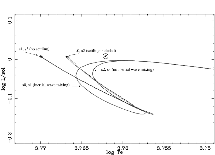
Figure 1: Evolutionary tracks for 1 $M_{\odot}$ stars with four variations on mixing physics. Model s0 includes gravitational settling/heavy element diffusion and inertial wave-driven mixing in radiative regions. Model s1 contains only wave mixing. Model s2 includes only settling/diffusion. Model s3 has no mixing outside of convective regions. Models with hydrodynamic mixing in radiative regions (s0 and s1) are indistinguishable on the pre-MS, when the shape of the track is controlled primarily by the size of the small convective core that exists during partial CN burning. Diffusion has insufficient time to work on the pre-MS and does not affect the tracks. On the main sequence, after the convective core disappears, the shape of the track is determined by the presence (s0 & s2) or absence (s1 & s3) of diffusion and settling.

4 ECLIPSING BINARIES

The double-lined eclipsing spectroscopic binaries in Andersen (1991) provide us with a sample of stars from $1M_{\odot}<M<23M_{\odot}$ with precisely determined masses and radii. A subset of these stars also have measured apsidal motions, which provide some information on the interior density profiles and core sizes of the stars. We use the same sample as Young, Mamajek, Arnett, & Liebert (2001) so that a direct comparison of the same code with and without complete descriptions of mixing physics outside of convective regions can be made. We use the most recent values available for observed quantities (observed quantities and references can be found in Table 3.)

As in Young, Mamajek, Arnett, & Liebert (2001), we calculate a $\chi^{2}$-like quantity for each binary pair, defined by

$$\chi^{2} = ((\log L(m_{A},t)-\log L_{A})/\sigma_{L}(A))^{2}$$ (10)

$$+ ((\log L(m_{B},t)-\log L_{B})/\sigma_{L}(B))^{2}$$

$$+ ((\log R(m_{A},t)-\log R_{A})/\sigma_{R}(A))^{2}$$

$$+ ((\log R(m_{B},t)-\log R_{B})/\sigma_{R}(B))^{2},$$

where $A$ and $B$ denote the primary and the secondary star, respectively. Here $L_{A}$ and $R_{A}$ are the observationally determined luminosity and radius of the primary, with $\sigma_{LA}$ and $\sigma_{RA}$ being the observational errors in $\log L_{A}$ and in $\log R_{A}$. We convert the observational data for the radii to logarithmic form for consistency. Correspondingly, $L(m_{A},t)$ and $R(m_{A},t)$ are the luminosity and radius of the model. This $\chi^{2}$ was evaluated by computing two evolutionary sequences, one for a star of mass $m_{A}$ and one for $m_{B}$. A $\chi^{2}$ was calculated at consistent times through the entire sequence ($t_{A}=t_{B}$ to a fraction of a time step, which was a relative error of a few percent at worst). The smallest $\chi^{2}$ value determined which pair of models was optimum for that binary. Note that if the trajectories of both $A$ and $B$ graze the error boxes at the same time, $\chi^{2}\approx 4$. We use radius instead of effective temperature in our fitting algorithm because the more precise values for $R$ make the $\chi^{2}$ more discriminating. These error parameters along with the corresponding uncertainties from the observations are presented in Table 4.

As before, we note that a $\chi^{2}$ statistic assumes that the observational errors have a Gaussian distribution about the mean (Press et al.,, 1992). This is not necessarily true, as the systematic shifts in measured quantities due to new analyses can be much larger than the formal error bars (Ribas et al., 2000; Stickland, Koch & Pfeiffer, 1992; Stickland, Lloyd, & Corcoran, 1994). Also, the quoted luminosity depends on the radius and effective temperature, and is thus not entirely independent. These systematic errors are the true limit to our power to discriminate between models, and emphasize the need for independent observational tests and numerical simulations to identify relevant physics.

Probably the greatest observational limitation we face is the lack of abundance determinations for these stars. The only binary in our original sample with a spectroscopic abundance determination is UX Men ($z$=0.019)(Andersen, Clausen, Magain, 1989). A few other systems have some sort of metallicity indication in the literature. Ribas et al. (2000) derive a metallicity of $z$=0.013 from fits to evolutionary tracks for the ever troublesome $\zeta$ Phe. Synthetic BaSeL photometry of VV Pyx suggests a metallicity of $z<$0.007, but the fits are not good (Lastennet et al., 1999). Latham et al. (1996) and Lastennet & Valls-Gabaud (2002) argue for a metal content similar to the Hyades in DM Vir ($z$=0.23). MY Cyg A&B and AI Hya A are all peculiar metal line stars. We (somewhat arbitrarily) also assign these systems a Hyades composition. AI Hya has a measured $z=0.07$, but this is probably a surface enhancement and does not reflect the global composition of the star (Ribas et al., 2000). Other systems either have no metallicity determinations or are sufficiently near solar composition that models of solar composition fall within the observational errors.

4.1 Global Properties of the Errors

The $\chi^{2}$ values for each binary pair with and without complete mixing physics are plotted in Figure 2. An arrow shows the shift in $\chi^{2}$ from baseline models to models with the full suite of physics. Fifteen of the binaries have excellent fits ($\chi^{2}<4$). Only three systems are marginal ($\zeta$ Phe, $\chi^{2}=4.10$; AI Hya, $\chi^{2}=4.12$; EK Cep, $\chi^{2}=5.97$). These systems will be discussed individually later. In all cases where the previous fits were marginal to poor, the $\chi^{2}$ improved. All massive binaries ($M_{A},M_{B}>4M_{\odot}$) with good fits also improved. Results were mixed for lower mass stars with good fits. In both of the latter groups, both complete and incomplete models fall within the observational errors, so there is little to distinguish between models for individual binaries. The threshold for rejection of a model with $\nu=4$ degrees of freedom with an $\alpha$ = 5% chance of rejecting a true hypothesis is $\chi^{2}=9.488$, so even the marginal fits do not give us a strong hold on remaining errors in our models. We must examine systematic discrepancies or wait for tighter observational error bars.

We show $\chi^{2}$ values for our best estimate of the metallicity. It is difficult to make a global statement about how metallicity affects the results of the tests, because it varies depending upon the characteristics of the binary. For the most massive binaries, a change in composition from solar ($z=0.0189$) to $z=0.004$ (roughly that of the Large Magellanic Cloud) results in a shift in the HR diagram roughly comparable to the observational errors. A similar shift in abundances for the lowest mass stars can shift the models well outside the region of good fit, primarily because of the smaller size of the observational errors rather than an intrinsic physical sensitivity. The converse is not necessarily true, however. AI Hya is the most extreme case. Using a solar composition model with complete mixing physics results in a $\chi^{2}=11.2$, because the model is too luminous at the correct $T_{eff}$. The converse situation does not hold. A solar composition model with only standard physics has $\chi^{2}>20$. A supersolar composition does not produce a significant improvement because the main sequence never travels far enough to the red for either case. Only increased mixing solves this problem. In general, it is safe to say that a change in metallicity of a factor of 2-4 is sufficient to move a binary model out of good agreement with observations. A similar change may or may not make poor model fit well. In order to pin down the stellar physics we must either examine systematic trends or find better abundance determinations.

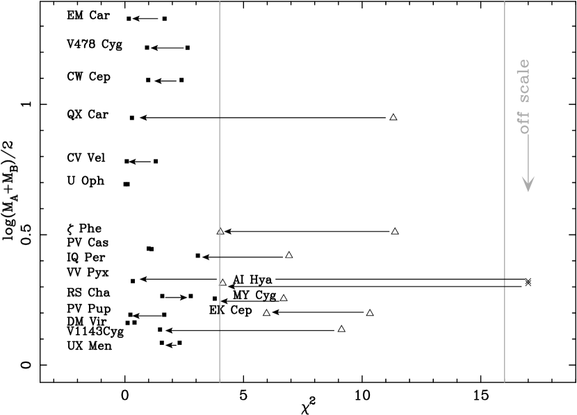
Figure 2: $\chi^{2}$ values for optimum models of binaries, versus mean mass of the binary. Arrows are drawn from Young, Mamajek, Arnett, & Liebert (2001) values to values for current models with more complete physics. The improvement is dramatic. The vertical line at $\chi^{2}=4$ indicates a fit in which the models are just within the observational errors for both stars.

Figure 3 shows goodness of fit vectors with the HR diagram for all stars in the sample, with incomplete models on the left and complete models on the right. The observed points with error bars are plotted with an arrow indicating distance and direction to the best fit model point. We can now begin to discriminate between models even for formally excellent fits. The most striking feature of the figure is the behavior of the massive stars ($M>4M_{\odot}$). The incomplete models are systematically underluminous. This suggests three possibilities: (1) the massive stars are all low metallicity; (2) the observational luminosity and/or mass determinations are systematically low; (3) the stars have larger convective cores than standard models predict. Option (1) is unlikely for nearby massive stars with ages of less than $10^{8}$ years, but cannot be absolutely ruled out without spectroscopic abundance determinations. Option 2 is possible, but again unlikely for a sample of 6 widely separated binaries. (Both EM Car and CW Cep have had their masses revised downward by Stickland, Koch & Pfeiffer (1992).) Option 3 seems the most likely, and is consistent with other evidence of mixing in stars beyond the standard model. Indeed, the trend virtually disappears when realistic mixing is included. It may be argued that the standard model is hydrodynamically inconsistent, as indicated by the instantaneous deceleration required at convective boundaries, and by detailed analysis of realistic high resolution 3-D hydrodynamic simulations, problems which our mixing algorithm addresses.

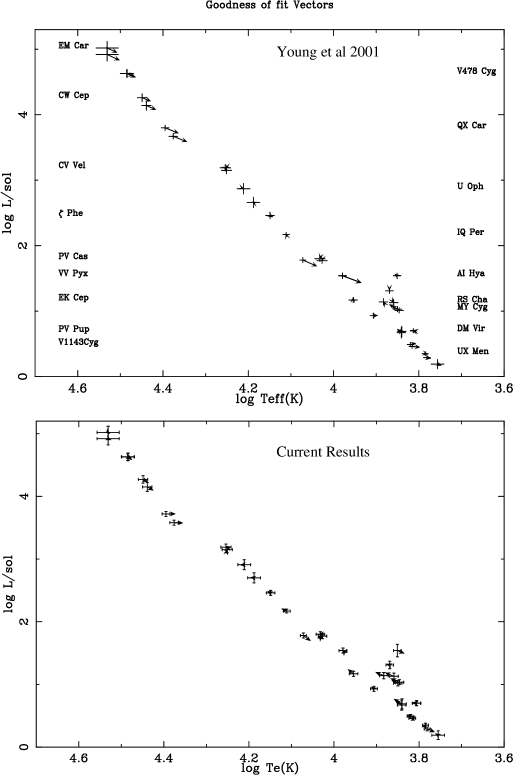
Figure 3: Goodness of fit vectors for each member of binary sample, with observational error bars. Young, Mamajek, Arnett, & Liebert (2001) results are on the top; present results on the bottom.

The salubrious effect of realistic mixing is confirmed by the apsidal motion tests. Models with incomplete mixing have systematically higher predicted apsidal motions in the four most massive systems. This indicates that the models are not sufficiently centrally condensed. (See Young, Mamajek, Arnett, & Liebert (2001) for a complete discussion of our previous results and methodology.) The current models with realistic mixing physics have larger convective cores and are therefore more centrally condensed. Table 5 summarizes the apsidal motion results for our binaries. Figure 4 shows the dimensionless rate of apsidal motion, $(P/U)_{CL}=(P/U)_{OBS}-(P/U)_{GR}$, which would be due to classical apsidal motion, plotted versus log of half the total binary mass (where $CL$ denotes classical and $GR$ general relativistic parts, and $OBS$ the observed motion). $P$ is the orbital period and $U$ the apsidal period. The observational data (corrected for general relativity) are shown as diamonds, with vertical error bars. All of the massive star models now fall within the error bars for the measured apsidal motion with the exception of QX Car, which differs by roughly two and a half sigma (insofar as sigma is a meaningful expression of these errors). QX Car does not differ from the measured point by a larger absolute amount than the other binaries; it simply has much tighter error bars. Either the observational uncertainties are underestimated or, equally likely, the models are still missing some physics. We have reanalyzed all of the binaries from EM Car to IQ Per. The lower mass binaries all have quoted apsidal motions smaller than the predicted general relativistic term. We find it more likely that there are errors in measuring an apsidal motion with periods of centuries than in weak-field general relativity.

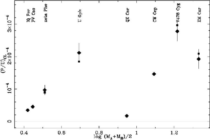
Figure 4: Classical apsidal motion versus mean mass, for our binaries with measured apsidal motion. $(P/U)_{CL}=(P/U)_{OBS}-(P/U)_{GR}$ is assumed. Diamonds are observed values, squares are model fits. Note that the symbol for QX Car is larger than error bars, and QX Car is not a good fit.

4.2 Individual Systems of Interest

4.2.1 $\zeta$ Phe

This system is perennially troublesome to stellar modelers (i.e. Ribas et al., 2000). It is difficult to fit both components with the same metallicity. We adopt $z=0.013$, following Ribas et al. (2000) and achieve a marginal fit ($\chi^{2}=4.026$). The secondary star is more luminous than the models when a good fit is achieved for the primary. If the observations are correctly interpreted, then the secondary model requires either a lower metallicity or enhanced mixing. Figure 5 shows the observed points and model tracks for $\zeta$ Phe.

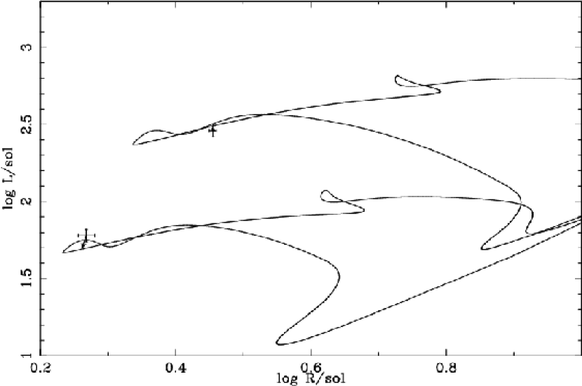
Figure 5: Evolutionary tracks ($z=0.013$) and observed points with errors for $\zeta$ Phe. Note that the secondary star is more luminous than the models when the primary is well fit.

4.2.2 AI Hya

AI Hya is identified as a peculiar metal line star (spectral class F2m). Its metallicity is measured as $z=0.07$ (Ribas et al., 2000), but this is probably due to a surface enhancement. Still, the stars are probably metal rich relative to solar. Without a precise determination of the interior composition we choose to use a Hyades composition ($z=0.023$) as being in the reasonable range of nearby metal rich compositions. In keeping with our effort to test the predictability of our code, we do not try to optimize the fit by further varying the composition. This system is particularly interesting in that increased metallicity alone cannot reconcile tracks with only convective mixing with the observations. The primary of the system lies farther redward in the HR diagram than the terminal age main sequence (Young, Mamajek, Arnett, & Liebert, 2001). The lifetime on the Hertzsprung gap for a 2 $M_{\odot}$ star is short. It is possible to catch a star in that stage, but unlikely, as $\tau_{gap}/\tau_{MS}<2\%$. More realistic mixing gives a larger convective core, extending the track redward so that a fit on the main sequence is easily achievable. Figure 6 shows the observed points and model tracks for AI Hya.

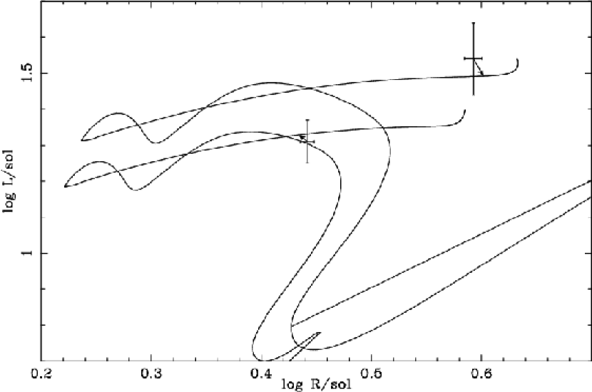
Figure 6: Evolutionary tracks ($z=0.023$) and observed points with errors for AI Hya. Realistic mixing allows an acceptable fit to this previously difficult pair.

4.2.3 EK Cep

EK Cep and RS Cha are both pre-MS systems (Popper, 1987; Mamajek, Lawson, & Feigelson, 2000). The fit to RS Cha is formally a good one ($\chi^{2}=2.776$), and we do not attempt to optimize within the observational errors. EK Cep, however, achieves only a marginal fit ($\chi^{2}=5.973$), because the radius of the secondary star is larger that that of the models during the first rise of the CN burning bump. (Other early pre-MS models show similar behavior, so we suspect this is systematic. A larger sample will be discussed in a forthcoming paper.) This is a robust behavior, in the sense that most things we could do to the models do not push them in the right direction. The non-convective mixing physics does not have a substantial effect, and increased metallicity would change the luminosity too much to result in a good fit. We can only find good agreement by reducing the mixing length parameter to $\alpha=1.6$. This suggests a change in the nature of the convection, but since $\alpha$ does not represent a physical entity, it does not tell us what that change is. We may speculate that since the star is trying to transport an amount of energy to a surface with a larger radius than a main sequence star of similar luminosity, the convective Mach numbers must be higher. This contributes a proportionally greater term to the stress tensor than main sequence convection and manifests as a radially directed pressure term, which would result in a larger radius for hydrostatic equilibrium. Besides this term, there are plasma effects, non-hydrogenic molecular contributions to the EOS, molecular and grain opacities, and subtleties of atmosphere models which must be taken into account which may contribute to the resolution of the problem. In short, we can identify a deficiency in our physics, and probably localize it to the physics of convection, but we do not have good predictive accuracy in this evolutionary stage. We quote the $\chi^{2}$ for our usual value of $\alpha=2.1$, and not the improved fit for $\alpha=1.6$, since this is not a predictable change. We plan 3-D simulations of convection in pre-MS and MS stars, which we hope will characterize the difference in the convection in a physical way. Figure 7 shows the observed points and model tracks for EK Cep.

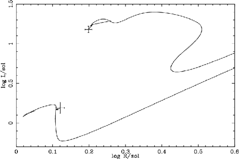
Figure 7: Evolutionary tracks ($z=0.019$) and observed points with errors for EK Cep. The models for the secondary star were run with a reduced mixing length parameter of $\alpha=1.6$ in order to increase the model radius to that of the observations. This indicates a change in the nature of the convection.

4.2.4 TZ For

TZ For was not in our original binary sample, but is a sufficiently interesting system that we examine it briefly here. The secondary is a subgiant in the Hertzsprung gap (Pols et al., 1997) with a spectroscopically determined metallicity of $z=0.024\pm 0.007$. Lastennet & Valls-Gabaud (2002) attempt to fit the secondary with several stellar evolution codes, but are unsuccessful without changing the mass of the model by 5$\sigma$ or using a composition not in agreement with the observations.Figure 8 shows the observed points and model tracks for TZ For.

Changing the size of the convective core on the main sequence necessarily changes the path the star takes across the Hertzsprung gap. We find that with realistic mixing, our models match the hotter component of TZ For reasonably well, and the cooler component exceptionally well. The models for the subgiant are slightly overluminous. We find a $\chi^{2}=0.77$ for the binary at $t=5.3\times 10^{8}$ yr. Virtually all of this discrepancy comes from the subgiant.

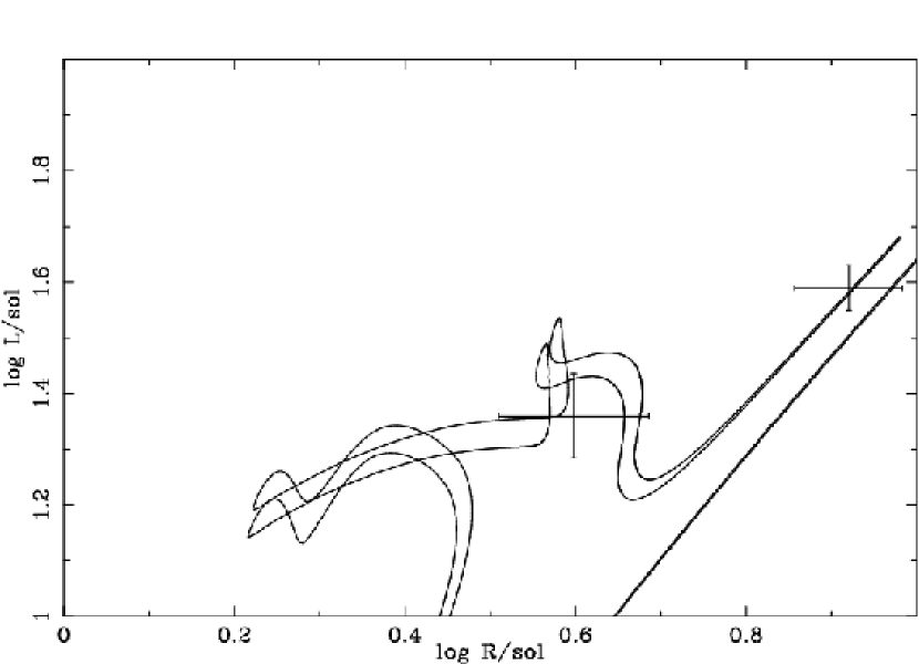
Figure 8: Evolutionary tracks ($z=0.024$) and observed points with errors for TZ For. The models are slightly overluminous with respect to the observed hot component, but much improved over standard models.

5 CONCLUSIONS

In this paper we test the predictive power of the TYCHO stellar evolution code against a set of classical observational tests. With an improved version of the realistic mixing physics presented in Young et al. (2003), we find excellent agreement with solar models and the sample of double-lined eclipsing binaries from Young, Mamajek, Arnett, & Liebert (2001). By avoiding optimization of our models with composition changes or parameterized extra mixing, we also identify several issues which are important to future development of stellar modeling.

From the solar models we find that our predictive accuracy for the sort of gross observables ($L,R,T_{eff}$) we measure for other stars is limited to of order 5-10% by (1) inadequacy in our description of convection, manifested by an uncertainty in the fictitious mixing length parameter, and (2) by uncertainties in abundances. If the nature of the convection is fixed by numerical simulations of full 3-D convection, the uncertainty is reduced to that arising from the abundance determinations. The good agreement of the neutrino fluxes with those of the standard model indicate that the influence of the mixing length description is an “atmospheric” effect. The rest of our (more or less parameter-free) physics provides a good description of the interior of the sun. We wish to emphasize that the quoted uncertainty is not a precise figure, but rather our best estimate, accounting for various known errors and incomplete physical descriptions. The sun is a well constrained system, and has uncomplicated physics compared to most other stars. In this light our measure of uncertainty should be taken as a best case for stellar evolution, with the caveat that errors can become substantially worse as we examine more complex, less well observed systems.

One of the most striking features of the solar models underlines a fundamental problem of stellar evolution. The two models that match observed solar quantities best have virtually identical tracks on the main sequence, which are shaped primarily by the inclusion of gravitational settling and diffusion of heavy elements. The models diverge significantly, however, on the pre-MS, where the influence of hydrodynamic mixing in radiative regions dominates the evolutionary pathway while the transient convective core is at its maximum extent. (Our theoretical treatment naturally predicts a smaller effect on the HR diagram for stars with smaller convective cores. This is consistent with the results of Michaud et al. (2004), which find minimal overshooting for the stars near the convective/radiative boundary in M67, a result which contradicts simple parameterized overshooting.) In at least some cases, a good fit to observations can be achieved without including physics which may be very important to the overall evolution. This may be adequate for describing the state of an individual star, but presents a serious problem for characterizing the behavior of a star or population over time.

The eclipsing binaries provide a test of our physics, particularly the more complete mixing, over a wide range of stellar masses. The systematic problems with massive star models, which were identified in Young, Mamajek, Arnett, & Liebert (2001), are ameliorated by the new treatment. The models are no longer underluminous, and the central condensations as measured by apsidal motions are no longer too small. Both of these improvements arise from larger convective core sizes resulting from the improved mixing. Simultaneously, the fits for almost all of the lower mass stars improve as well. The one case in which the error formally increases varies within the observational errors. All of the poor or marginal fits in Young, Mamajek, Arnett, & Liebert (2001) improve dramatically. Some of the improvement in these lower mass models arises from the use of non-solar abundances in a few cases, but the composition alone cannot account for all of the error in the earlier models. AI Hya is a particularly fine example, for the higher mass star lies redward of the TAMS in models with incomplete mixing physics, a situation which metallicity cannot help. More mixing is necessary for good agreement. We do not optimize our models by varying composition. It is changed only when an abundance estimate appears in the literature.

Further insight into potential pitfalls can be found in the binary sample. An increase in metallicity moves the tracks in the opposite sense of more complete mixing. It is possible to achieve an equally good fit with low metallicity and incomplete mixing or higher metallicity and more realistic physics. The practice of making stellar abundance determinations by fitting evolutionary tracks is dangerous unless the physics in the code is very well tested independently. It is vital that accurate spectroscopic abundance determinations be made for stars used as test cases of stellar evolution, particularly eclipsing binaries.

The pre-MS systems identify an area where our physics is still inadequate. Our predictive accuracy for these systems is not satisfactory. We must make an ad hoc adjustment to the mixing length in order to get large enough model radii. This tells us that our description of convection is insufficiently physical. Further multidimensional simulations of envelope convection in low surface gravity stars is necessary to resolve this problem.

When coupled with the observational tests of light element depletion and turnoff ages in young clusters in Young et al. (2003) we explore the performance of TYCHO on stars with both convective and radiative cores and convective envelopes of various sizes on the pre-MS and main sequence. All of these tests are performed with the same physics. No changes are made to the mixing or composition in order to improve our agreement with the observations. We find a strong increase in the predictive (as opposed to calibrated) accuracy throughout this range of conditions. This is of course a small sub-set of problems in stellar astrophysics, but we have increasing confidence in extending the approach to problems in other areas of stellar evolution. In the future we plan to examine the impact of this new approach on AGB nucleosynthesis, nucleosynthesis in very low metallicity and evolved massive stars, and the evolution of extremely massive stars which become luminous blue variables and SNIb/c progenitors.

Table 3: Observed parameters for selected binary systems.

System	P(d)	Star	Spect.	Mass/$M_{\odot}$	Radius/$R_{\odot}$	$\log g{\rm(cm/s^{2})}$	$\log T_{e}{\rm(K)}$	$\log L/L_{\odot}$
EM Car	$3.41$	A	O8V	$22.3\pm 0.3$	$9.34\pm 0.17$	$3.864\pm 0.017$	$4.531\pm 0.026$	$5.02\pm 0.10$
HD97484	$\cdots$	B	O8V	$20.3\pm 0.3$	$8.33\pm 0.14$	$3.905\pm 0.016$	$4.531\pm 0.026$	$4.92\pm 0.10$
V478 Cyg	$2.88$	A	O9.5V	$16.67\pm 0.45$	$7.423\pm 0.079$	$3.919\pm 0.015$	$4.484\pm 0.015$	$4.63\pm 0.06$
HD193611	$\cdots$	B	O9.5V	$16.31\pm 0.35$	$7.423\pm 0.079$	$3.909\pm 0.013$	$4.485\pm 0.015$	$4.63\pm 0.06$
CW Cep	$2.73$	A	B0.5V	$12.9\pm 0.1$	$5.685\pm 0.130$	$4.039\pm 0.024$	$4.449\pm 0.011$	$4.26\pm 0.06$
HD218066	$\cdots$	B	B0.5V	$11.9\pm 0.1$	$5.177\pm 0.129$	$4.086\pm 0.024$	$4.439\pm 0.011$	$4.14\pm 0.07$
QX Car	$4.48$	A	B2V	$9.267\pm 0.122$	$4.289\pm 0.091$	$4.140\pm 0.020$	$4.395\pm 0.009$	$3.80\pm 0.04$
HD86118	$\cdots$	B	B2V	$8.480\pm 0.122$	$4.051\pm 0.091$	$4.151\pm 0.021$	$4.376\pm 0.010$	$3.67\pm 0.04$
CV Vel	$6.89$	A	B2.5V	$6.100\pm 0.044$	$4.087\pm 0.036$	$4.000\pm 0.008$	$4.254\pm 0.012$	$3.19\pm 0.05$
HD77464	$\cdots$	B	B2.5V	$5.996\pm 0.035$	$3.948\pm 0.036$	$4.023\pm 0.008$	$4.251\pm 0.012$	$3.15\pm 0.05$
U Oph	$1.68$	A	B5V	$5.198\pm 0.113$	$3.438\pm 0.044$	$4.081\pm 0.015$	$4.211\pm 0.015$	$2.87\pm 0.08$
HD156247	$\cdots$	B	B6V	$4.683\pm 0.090$	$3.005\pm 0.055$	$4.153\pm 0.018$	$4.188\pm 0.015$	$2.66\pm 0.08$
$\zeta$ Phe	$1.67$	A	B6V	$3.930\pm 0.045$	$2.851\pm 0.015$	$4.122\pm 0.009$	$4.149\pm 0.010$	$2.46\pm 0.04$
HD6882	$\cdots$	B	B8V	$2.551\pm 0.026$	$1.853\pm 0.023$	$4.309\pm 0.012$	$4.072\pm 0.007$	$1.78\pm 0.04$
IQ Per	1.74	A	B8V	$3.521\pm 0.067$	$2.446\pm 0.026$	$4.208\pm 0.019$	$4.111\pm 0.008$	$2.17\pm 0.03$
HD24909	$\cdots$	B	A6V	$1.737\pm 0.031$	$1.503\pm 0.017$	$4.323\pm 0.013$	$3.906\pm 0.008$	$0.93\pm 0.04$
PV Cas	1.75	A	B9.5V	$2.815\pm 0.050$	$2.297\pm 0.035$	$4.165\pm 0.016$	$4.032\pm 0.010$	$1.80\pm 0.04$
HD240208	$\cdots$	B	B9.5V	$2.756\pm 0.054$	$2.257\pm 0.035$	$4.171\pm 0.016$	$4.027\pm 0.010$	$1.77\pm 0.04$
AI Hya	8.29	A	F2m	$2.145\pm 0.038$	$3.914\pm 0.031$	$3.584\pm 0.011$	$3.851\pm 0.009$	$1.54\pm 0.02$
+0°2259	$\cdots$	B	F0V	$1.978\pm 0.036$	$2.766\pm 0.017$	$3.850\pm 0.010$	$3.869\pm 0.009$	$1.31\pm 0.02$
VV Pyx	4.60	A	A1V	$2.101\pm 0.022$	$2.167\pm 0.020$	$4.089\pm 0.009$	$3.979\pm 0.009$	$1.54\pm 0.04$
HD71581	$\cdots$	B	A1V	$2.099\pm 0.019$	$2.167\pm 0.020$	$4.088\pm 0.009$	$3.979\pm 0.009$	$1.54\pm 0.04$
RS Cha	1.67	A	A8V	$1.858\pm 0.016$	$2.137\pm 0.055$	$4.047\pm 0.023$	$3.883\pm 0.010$	$1.14\pm 0.05$
HD75747	$\cdots$	B	A8V	$1.821\pm 0.018$	$2.338\pm 0.055$	$3.961\pm 0.021$	$3.859\pm 0.010$	$1.13\pm 0.05$
EK Cep	4.43	A	A1.5V	$2.029\pm 0.023$	$1.579\pm 0.007$	$4.349\pm 0.010$	$3.954\pm 0.010$	$1.17\pm 0.04$
HD206821	$\cdots$	B	G5Vp	$1.124\pm 0.012$	$1.320\pm 0.015$	$4.25\pm 0.010$	$3.756\pm 0.015$	$0.19\pm 0.07$
TZ For	75.67	A	F6IV	$1.949\pm 0.022$	$3.96\pm 0.09$	$3.532\pm 0.02$	$3.803\pm 0.007$	$1.36\pm 0.06$
HD20301	$\cdots$	B	G8III	$2.05\pm 0.06$	$8.32\pm 0.12$	$2.91\pm 0.017$	$3.699\pm 0.009$	$1.59\pm 0.04$
MY Cyg	4.01	A	F0m	$1.811\pm 0.030$	$2.193\pm 0.050$	$4.007\pm 0.021$	$3.850\pm 0.010$	$1.03\pm 0.04$
HD193637	$\cdots$	B	F0m	$1.786\pm 0.025$	$2.193\pm 0.050$	$4.014\pm 0.021$	$3.846\pm 0.010$	$1.02\pm 0.04$
PV Pup	1.66	A	A8V	$1.565\pm 0.011$	$1.542\pm 0.018$	$4.257\pm 0.010$	$3.870\pm 0.01$	$0.81\pm 0.08$
HD62863	$\cdots$	B	A8V	$1.554\pm 0.013$	$1.499\pm 0.018$	$4.278\pm 0.011$	$3.870\pm 0.01$	$0.79\pm 0.08$
DM Vir	4.67	A	F7V	$1.454\pm 0.008$	$1.763\pm 0.017$	$4.108\pm 0.009$	$3.813\pm 0.007$	$0.67\pm 0.03$
HD123423	$\cdots$	B	F7V	$1.448\pm 0.008$	$1.763\pm 0.017$	$4.106\pm 0.009$	$3.813\pm 0.020$	$0.67\pm 0.03$
V1143 Cyg	7.64	A	F5V	$1.391\pm 0.016$	$1.346\pm 0.023$	$4.323\pm 0.016$	$3.820\pm 0.007$	$0.49\pm 0.03$
HD185912	$\cdots$	B	F5V	$1.347\pm 0.013$	$1.323\pm 0.023$	$4.324\pm 0.016$	$3.816\pm 0.007$	$0.46\pm 0.03$
UX Men	4.18	A	F8V	$1.238\pm 0.006$	$1.347\pm 0.013$	$4.272\pm 0.009$	$3.789\pm 0.007$	$0.38\pm 0.03$
HD37513	$\cdots$	B	F8V	$1.198\pm 0.007$	$1.274\pm 0.013$	$4.306\pm 0.009$	$3.781\pm 0.007$	$0.32\pm 0.03$

Table 4: Results for selected binary systems.

System	Star	Mass	$\log R/R_{\odot}$	$\log T_{e}$	$\log L$	log Age (yr)	$z$	$\chi^{2}$
EM Car	A	$22.30$	0.969	4.526	4.996	6.075	0.0189	0.16
HD97484	B	$20.30$	0.926	4.523	4.898	6.076
V478 Cyg	A	$16.71$	0.881	4.476	4.618	6.310	0.0189	0.93
HD193611	B	$16.31$	0.865	4.474	4.580	6.312
CW Cep	A	$12.90$	0.764	4.437	4.228	6.404	0.0189	0.98
HD218066	B	$11.90$	0.722	4.424	4.093	6.406
QX Car	A	9.267	0.640	4.372	3.721	6.531	0.0189	0.30
HD86118	B	8.480	0.602	4.354	3.576	6.563
CV Vel	A	6.100	0.609	4.255	3.193	7.295	0.0189	0.08
HD77464	B	5.996	0.602	4.251	3.159	7.299
U Oph	A	5.198	0.535	4.221	2.906	7.379	0.0189	0.03
HD156247	B	4.683	0.484	4.197	2.708	7.380
$\zeta$ Phe	A	3.930	0.455	4.157	2.490	7.703	0.013	4.03
HD6882	B	2.551	0.261	4.055	1.693	7.728
IQ Per	A	3.521	0.382	4.124	2.211	7.547	0.0189	3.07
HD24909	B	1.737	0.180	3.913	0.965	7.547
PV Cas	A	2.827	0.348	4.037	1.797	6.490	0.0189	1.00
HD240208	B	2.768	0.357	4.027	1.772	6.491
AI Hya	A	2.145	0.602	3.834	1.492	8.556	0.023	4.12
$+0\arcdeg 2259$	B	1.978	0.434	3.877	1.329	8.558
VV Pyx	A	2.101	0.339	3.981	1.555	8.610	0.007	0.33
HD71581	B	2.099	0.339	3.980	1.553	8.612
RS Cha	A	1.858	0.317	3.903	1.198	6.866	0.0189	2.78
HD75747	B	1.821	0.358	3.880	1.189	6.867
EK Cep	A	2.029	0.209	3.968	1.242	7.357	0.0189	5.13
HD206821	B	1.124	0.108	3.749	0.165	7.357
TZ For	A	1.95	0.552	3.818	1.428	8.713	0.024	0.77
HD20301	B	2.05	0.920	3.700	1.331	8.724
MY Cyg	A	1.811	0.337	3.867	1.095	8.649	0.023	3.79
HD193637	B	1.786	0.327	3.865	1.066	9.651
PV Pup	A	1.565	0.184	3.872	0.810	8.520	0.0189	0.23
HD62863	B	1.554	0.180	3.871	0.795	8.527
DM Vir	A	1.460	0.249	3.816	0.714	9.149	0.023	0.41
HD123423	B	1.454	0.243	3.817	0.706	9.149
V1143 Cyg	A	1.391	0.128	3.826	0.515	8.739	0.0189	1.48
HD185912	B	1.347	0.109	3.819	0.446	8.754
UX Men	A	1.238	0.134	3.795	0.400	9.542	0.021	1.56
HD37513	B	1.198	0.096	3.795	0.323	9.544

Table 5: Apsidal comparisons for selected binary systems.

System	Star	Mass	$-\log k_{i}$	$(k_{2}R^{5})$	$\rm P/U_{CL}$	$\rm P/U_{GR}$	$\rm P/U_{CL+GR}$	$\rm P/U_{OBS}$
EM Car	A	$22.3$	1.920	$347.0$	$2.091$	$0.275$	2.37	$2.2\pm 0.3$
	B	$20.3$	1.935	$267.5$
V478 Cyg	A	$16.67$	1.935	$160.6$	$2.97$	$0.223$	3.19	$3.0\pm 0.3$
	B	$16.31$	1.917	$140.0$
CW Cep	A	$12.90$	$1.878$	$49.50$	$1.46$	$0.178$	1.63	$1.640\pm 0.014$
	B	$11.90$	$1.894$	$32.11$
QX Car	A	$9.267$	$1.898$	$13.97$	$0.156$	$0.170$	0.326	$0.340\pm 0.006$
	B	$8.480$	$1.936$	$10.58$
U Oph	A	$5.198$	$2.124$	$2.687$	$1.85$	$0.0827$	1.93	$2.2\pm 0.3$
	B	$4.683$	$2.111$	$1.571$
$\zeta$ Phe	A	$3.930$	$2.308$	$1.025$	$0.894$	$0.0624$	0.956	$1.03\pm 0.15$
	B	$2.551$	$2.333$	$0.2018$
IQ Per	A	$3.521$	$2.278$	$0.4478$	$0.335$	$0.0553$	0.410	$0.40\pm 0.03$
	B	$1.737$	$2.416$	$0.0401$
PV Cas	A	$2.815$	$2.149$	$0.2012$	$0.414$	$0.0572$	0.499	$0.510\pm 0.011$
	B	$2.756$	$2.221$	$0.2375$

References

- Alexander & Ferguson (1994) Alexander, D. R. & Ferguson, J. W. 1994, ApJ, 437, 879
- Andersen (1991) Andersen, J. 1991, ARA&A, 3, 91
- Andersen, Clausen, Magain (1989) Andersen, J., Clausen, J. V., & Magain, P. 1989, A&A, 211, 346
- Asida (2000) Asida, S. M. 2000, ApJ, 528, 896
- Bahcall & Pinsonneault (2004) Bahcall, J. N. & Pinsonneault, M. H. 2004, Phys. Rev. Lett., 92, 121301
- Basu, Pinsonneault, & Bahcall (2000) Basu, S., Pinsonneault, M. H., & Bahcall, J. N., 2000, ApJ, 529, 1084
- Bahcall, Pinsonneault, & Basu (2001) Bahcall, J. N., Pinsonneault, M. H., & Basu, S. 2001, ApJ, 555, 990
- Blöcker (1995) Blöcker, T. 1995, A&A, 297, 727
- Boothroyd & Sackmann (2003) Boothroyd, A. I. & Sackmann, I.-J. 2003, ApJ, 583, 1004
- Caughlan & Fowler (1988) Caughlan, G., & Fowler, W. A., 1988, Atomic and Nuclear Data Tables, 40, 283
- Charbonnel & Talon (1999) Charbonnel, C., & Talon, S., 1999, A&A, 351, 635
- Chaboyer, Demarque, & Pinsonneault (1995) Chaboyer, B. Demarque, P., & Pinsonneault, M. H. 1995, ApJ, 441, 865
- Cox (1980) Cox, J. P., 1980, Theory of Stellar Pulsations, Princeton University Press, Princeton NJ
- Dupree & Reimers (1987) Dupree, A. K. & Reimers, D. 1987, in Exploring the Universe in the Ultraviolet with the IUE Satellite, eds. Y. Kondo et al. (Dordrecht: Reidel), p.231
- Feuchtinger, Buchler, & Kolláth (2000) Feuchtinger, M., Buchler, J. R., & Kolláth, Z. 200, ApJ, 544, 1056
- Grevesse & Sauval (1998) Grevesse, N. & Sauval, A. J., 1998, Space Science Reviews, 85, 161
- Hansen & Kawaler (1994) Hansen, C. J., & Kawaler, S. D., 1994, Stellar Interiors, Springer-Verlag
- Hillenbrand & White (2004) Hillenbrand, L. A. & White, R. J. 2004, ApJ, 604, 741
- Iglesias & Rogers (1996) Iglesias, C. & Rogers, F. J. 1996, ApJ, 464, 943
- Kippenhahn & Weigert (1990) Kippenhahn, R. & Weigert, A. 1990, Stellar Structure and Evolution, Springer-Verlag
- Kudritzki et al. (1989) Kudritzki, R. P., Pauldrach, A., Puls, J., Abbott, & D. C. 1989 A&A, 219, 205
- Lamers & Nugis (2003) Lamers, H. J. G. L. M. & Nugis, T. 2003 A&A, 395L, 1
- Lastennet & Valls-Gabaud (2002) Latennet, E. & Valls-Gabaud, D. 2002, A&A, 396, 551
- Lastennet et al. (1999) Lastennet, E., Lejeune, T., Westera, P., & Buser, R. 1999, A&A, 341, 857
- Latham et al. (1996) Latham, D. W., Nordström, B., Andersen, J., Torres, G., Stefanik, R. P., Thaller, M., & Bester, M. J. 1996, A&A, 314, 864
- Ledoux (1974) Ledoux, P. 1974, in IAU Symposium 59, Stellar Instability and Evolution, ed. P. Ledoux et al. (Dordrecht: Reidel)
- Lighthill (1978) Lighthill, J. 1978, Waves in Fluids (Cambridge: Cambridge University Press)
- Lodders (2003) Lodders, K., 2003, ApJ, 591, 1220
- Mamajek, Lawson, & Feigelson (2000) Mamajek, E. E., Lawson, W. A., & Feigelson, E. D. 2000, AJ, 112, 276
- Michaud et al. (2004) Michaud, G., Richard, O., Richer, J., & VandenBerg, D. A. 2004, ApJ, 606, 452
- Pinsonneault et al. (2002) Pinsonneault, M. H., Steigman, G., Walker, T. P., & Narayanan, V. K. 2002, ApJ, 574, 398
- Pols et al. (1997) Pols, O. R., Tout, C. A., Schröder, K-P., Eggleton, P. P., & Manners, J. 1997, MNRAS, 289, 869
- Popper (1987) Popper, D. M. 1987, ApJ, 313, L81
- Press et al., (1992) Press, W. H., Teukolsky, S. A., Vetterling, W. T., & Flannery, B. P., 1992, Numerical Recipes in FORTRAN, Second Edition, University Press: Cambridge
- Press (1981) Press, W. H. 1981, ApJ, 245, 286
- Press & Rybicki (1981) Press, W. H. & Rybicki, G. 1981, ApJ, 248, 751
- Rauscher & Thielemann (2000) Rauscher, T., & Thielemann, K.-F., 2000, Atomic Data Nuclear Data Tables, 75, 1
- Ribas et al. (2000) Ribas, I., Jordi, C., Torra, J., & Giménez, Á. 2000, MNRAS, 313, 99
- Robinson et al. (2004) Robinson, F. J., Demarque, P., Li, L. H., Sofia, S., Kim, Y.-C., Chan, K. L., & Guenther, D. B. 2004, MNRAS, 347, 1208
- Stassun et al. (2004) Stassun, K. G. Stassun, Mathieu, R. D., Vaz, L. P. R. , Stroud, N., & Vrba, F. J. 2004, ApJS, 151, 357
- Stickland, Koch & Pfeiffer (1992) Stickland, D. J., Koch, R. H., & Pfeiffer, R. J., 1992, Obs., 112, 277
- Stickland, Lloyd, & Corcoran (1994) Stickland, D. J., Lloyd, C., Corcoran, M. F., 1994, Obs., 114, 284
- Talon, Kumar, & Zahn (2002) Talon, S., Kumar, P., & Zahn, J-P., 2002, ApJ, 574, L175
- Tassoul (2000) Tassoul, J.-L. 2000, Stellar Rotation, Cambride University Press, NY
- Thoul, Bahcall, & Loeb (1994) Thoul, A. A., Bahcall, J. N., & Loeb, A. 1994, ApJ, 421, 828
- Timmes & Swesty (2000) Timmes, F. X. & Swesty, F. D. 2000, ApJS, 126, 501
- Young et al. (2003) Young, P. A., Knierman, K. A., Rigby, J. R., & Arnett, D. 2003, ApJ, 595, 1114
- Young, Mamajek, Arnett, & Liebert (2001) Young, P. A., Mamajek, E. E., Arnett, D., & Liebert, J. 2001, ApJ, 556, 230